
A Method of Enhancing Rapidly-Exploring Random Tree Robot Path Planning Using Midpoint Interpolation


Abstract
:1. Introduction
2. Related Works
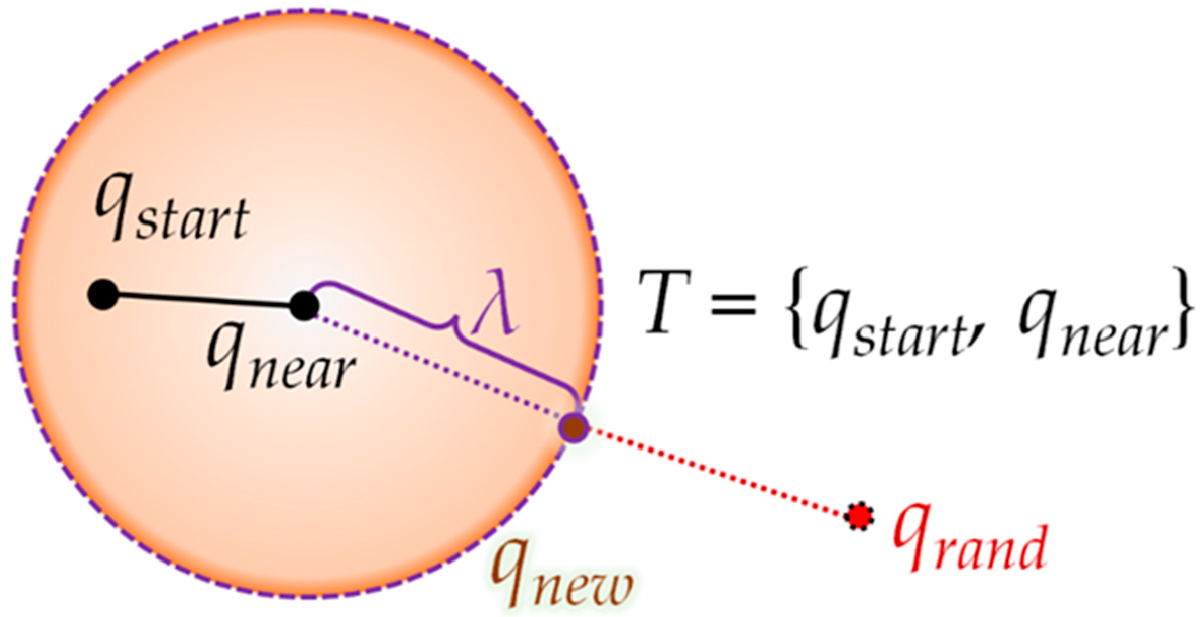
2.1. RRT
| Algorithm 1 Pseudocode of RRT Algorithm | |
| Input: | |
| qstart ← start point | |
| qgoal ← goal point | |
| λ ← step length | |
| C ← position set of all (measured) boundary points in all (known) obstacles | |
| N ← number of random samples | |
| Output: | |
| R ← result of path R | |
| Initialize: | |
| T ← Null tree<node, edge> | |
| ProcedureRRT | |
| Begin | |
| 1 | T ← Insert root node<qstart> to T |
| 2 | Whilen ← 0 To N Do |
| 3 | Generate n-th random sample |
| 4 | qrand ← position of n-th random sample |
| 5 | qnear ← position of the nearest node in T from qrand |
| 6 | If not isInside(qnear, qrand, λ) Then |
| 7 | qnew ← intersection point between line segment connecting qrand and qnear, and circle with radius λ centered at qnear |
| 8 | Else qnew ← qrand |
| 9 | If not isTrapped(qnew, qnear, C) Then |
| 10 | T ← Insert node<qnew> and edge<qnew, qnear> to T |
| 11 | If isInside(qnew, qgoal, λ) Then |
| 12 | T ← Insert node<qgoal> and edge<qnew, qgoal> to T |
| 13 | P ← path from last inserted node{qgoal} to root node{qstart} in T |
| 14 | If [length of R] > [length of P] Then R ← P |
| 15 | T ← Delete node<qgoal> and edge<qnew, qgoal> from T |
| End | |
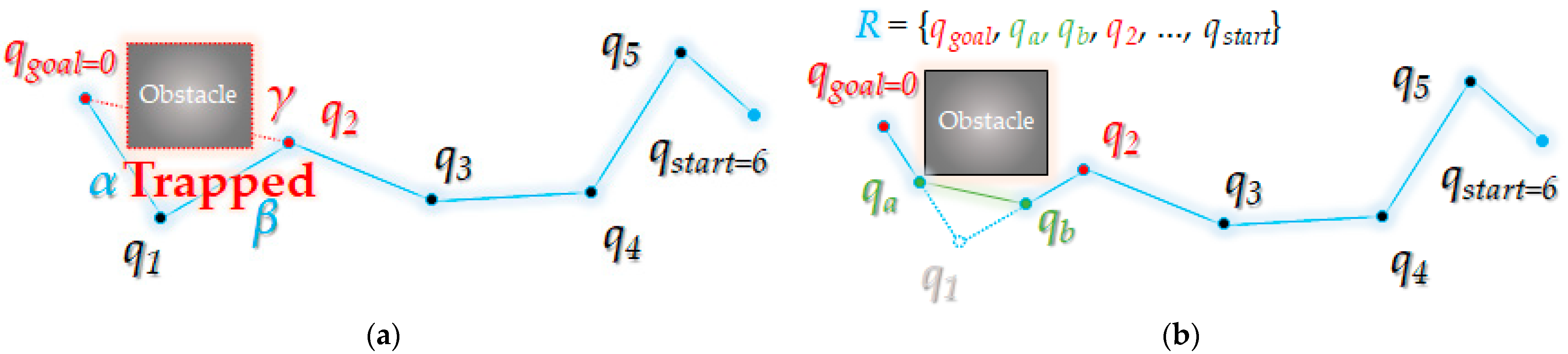
2.2. Triangular Rewiring Method for the RRT Algorithm
| Algorithm 2 Pseudocode of Triangular Rewiring Method for RRT Algorithm | |
| Input: | |
| qchild ← Position {qnew/qnewA/qnewB} | |
| qparent ← Position qnear | |
| T ← Tree {Tmerged/Ta/Tb} | |
| C ← Position Set C | |
| Output: | |
| {Tmerged/Ta/Tb} ← Result of T | |
| Begintriangular RewiringProcedure | |
| 1 | qancestor ← Position of Parent Node of qparent in T |
| 2 | If NotisTrapped(qancestor, qchild, C) then |
| 3 | T ← Delete Node<qparent>, Edge<qparent, qchild> and Edge<qparent, qancestor> from T |
| 4 | qparent ← qancestor |
| 5 | qancestor ← Position of Parent Node of qancestor in T |
| 6 | While Not qancestor = Null do |
| 7 | If Not isTrapped(qancestor, qchild, C) then |
| 8 | T ← Delete Node<qparent> and Edge<qparent, qancestor> from T |
| 9 | qparent ← qancestor |
| 10 | qancestor ← Position of Parent Node of qancestor in T |
| 11 | Else |
| 12 | Break |
| 13 | T ← Insert Edge<qparent, qchild> to T |
| 14 | Else |
| 15 | T ← Insert Node<qchild> and Edge<qchild, qparent> to T |
| Endtriangular RewiringProcedure | |
3. Proposed Post Triangular Processing of the Midpoint Interpolation Method
- The destination point may change gradually over time, but there is only one start point and one destination point for each tree.
- If the mobile robot cannot perform the omnidirectional motion, local planning or kinodynamic planning is performed separately on the path planning result.
| Algorithm 3 Pseudocode of Proposed Post Triangular Processing of Midpoint Interpolation Method | |
| Input: | |
| R ← path from {RRT/ …} | |
| C ← position set of all (measured) boundary points in all (known) obstacles | |
| ε ← threshold value of minimum clearance | |
| Output: | |
| R ← modified path R | |
| Initialize: | |
| fmodify ← true | |
| ProcedurepostTriProcOfMidInterpolation | |
| Begin | |
| 1 | WhilefmodifyDo |
| 2 | fmodify ← false // is the path modified |
| 3 | t ← 0 // index of the currently focused point |
| 4 | qchild ← first point in R |
| 5 | qparent ← next point of qchild in R |
| 6 | While not [qparent is the last point in R] Do |
| 7 | qancestor ← next point of qparent in R |
| 8 | If not isTrapped(qchild, qancestor, C) Then |
| 10 | R ← postTriangular(R, ε, t, fmodify) |
| 11 | Else |
| 12 | R ← interpolation(R, C, ε, t, fmodify) |
| 13 | qchild ← t-th point in R |
| 14 | qparent ← next point of qchild in R |
| End | |
| Algorithm 4 Pseudocode of Proposed Post Triangular Function | |
| Input: | |
| R ← path R from postTriProcOfMidInterpolation | |
| t ← point index t from postTriProcOfMidInterpolation | |
| fmodify ← boolean fmodify from postTriProcOfMidInterpolation | |
| Output: | |
| R ← modified path R | |
| fmodify ← result of boolean fmodify //return by reference | |
| Procedure postTriangular From postTriProcOfMidInterpolation | |
| Begin | |
| 1 | qchild ← t-th point in R |
| 2 | qparent ← next point of qchild in R |
| 3 | qancestor ← next point of qparent in R |
| 4 | R ← Delete path<qchild, qparent> and path<qparent, qancestor> from R |
| 5 | R ← Insert path<qchild, qancestor> to R |
| 6 | fmodify ← true |
| End | |
| Algorithm 5 Pseudocode of Proposed Interpolation Function | |
| Input: | |
| R ← path R from postTriProcOfMidInterpolation | |
| C ← position set C from postTriProcOfMidInterpolation | |
| ε ← threshold value ε from postTriProcOfMidInterpolation | |
| t ← point index t from postTriProcOfMidInterpolation | |
| fmodify ← boolean fmodify from postTriProcOfMidInterpolation | |
| Output: | |
| R ← modified path R | |
| t ← updated point index t // return by reference | |
| fmodify ← result of boolean fmodify // return by reference | |
| Initialize: | |
| qchild ← t-th point in R | |
| qparent ← next point of qchild in R | |
| qancestor ← next point of qparent in R | |
| ProcedureinterpolationFrompostTriProcOfMidInterpolation | |
| Begin | |
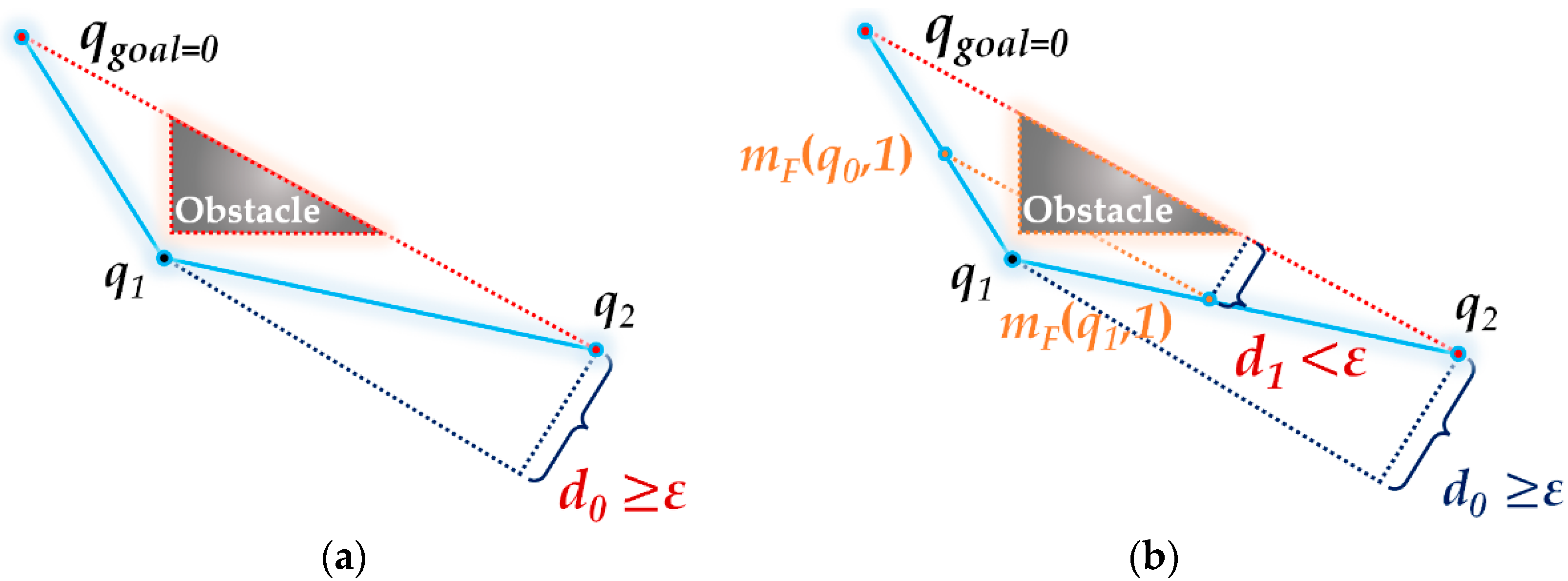
| 1 | d ← altitude of the triangle consisting of qchild, qparent, and qancestor with base <qchild, qancestor> |
| 2 | ma ← midpoint between qchild and qparent |
| 3 | mb ← midpoint between qparent and qancestor |
| 4 | While true Do |
| 5 | If d >= ε Then |
| 6 | If not isTrapped(ma, mb, C) Then |
| 7 | R ← Delete path<qchild, qparent> and path<qparent, qancestor> from R |
| 8 | R ← Insert path<qchild, ma>, path<ma, mb>, and path<mb, qancestor> to R |
| 9 | fmodify ← true |
| 10 | Break |
| 11 | Else |
| 12 | d ← d / 2 |
| 13 | ma ← midpoint between ma and qparent |
| 14 | mb ← midpoint between mb and qparent |
| 15 | Else |
| 16 | t ← t + 1 |
| 17 | Break |
| End | |
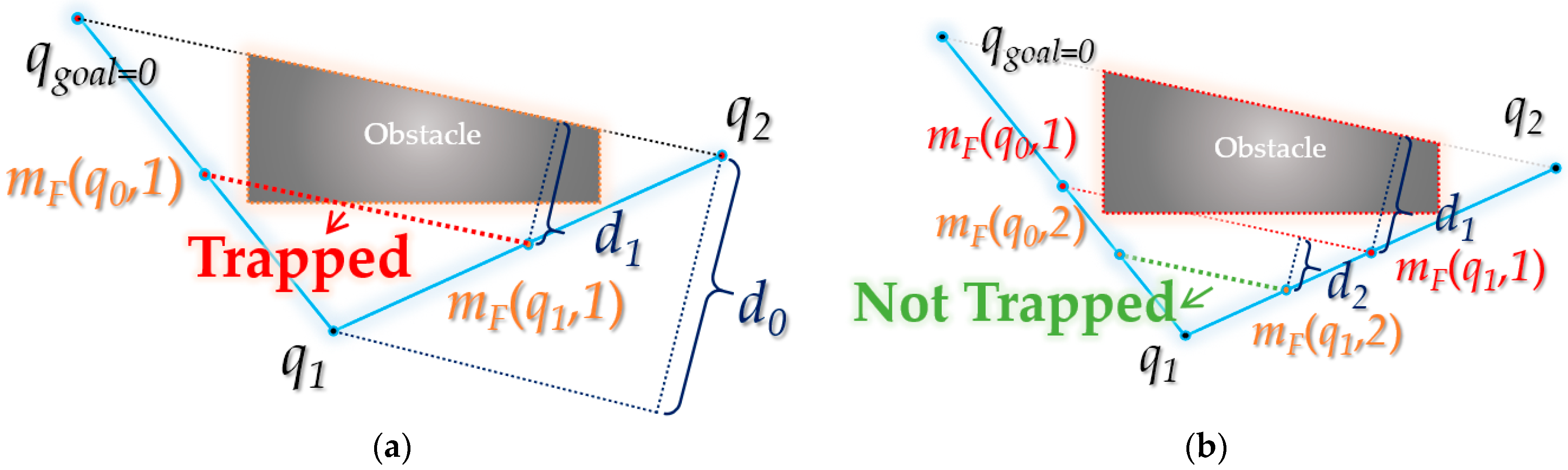
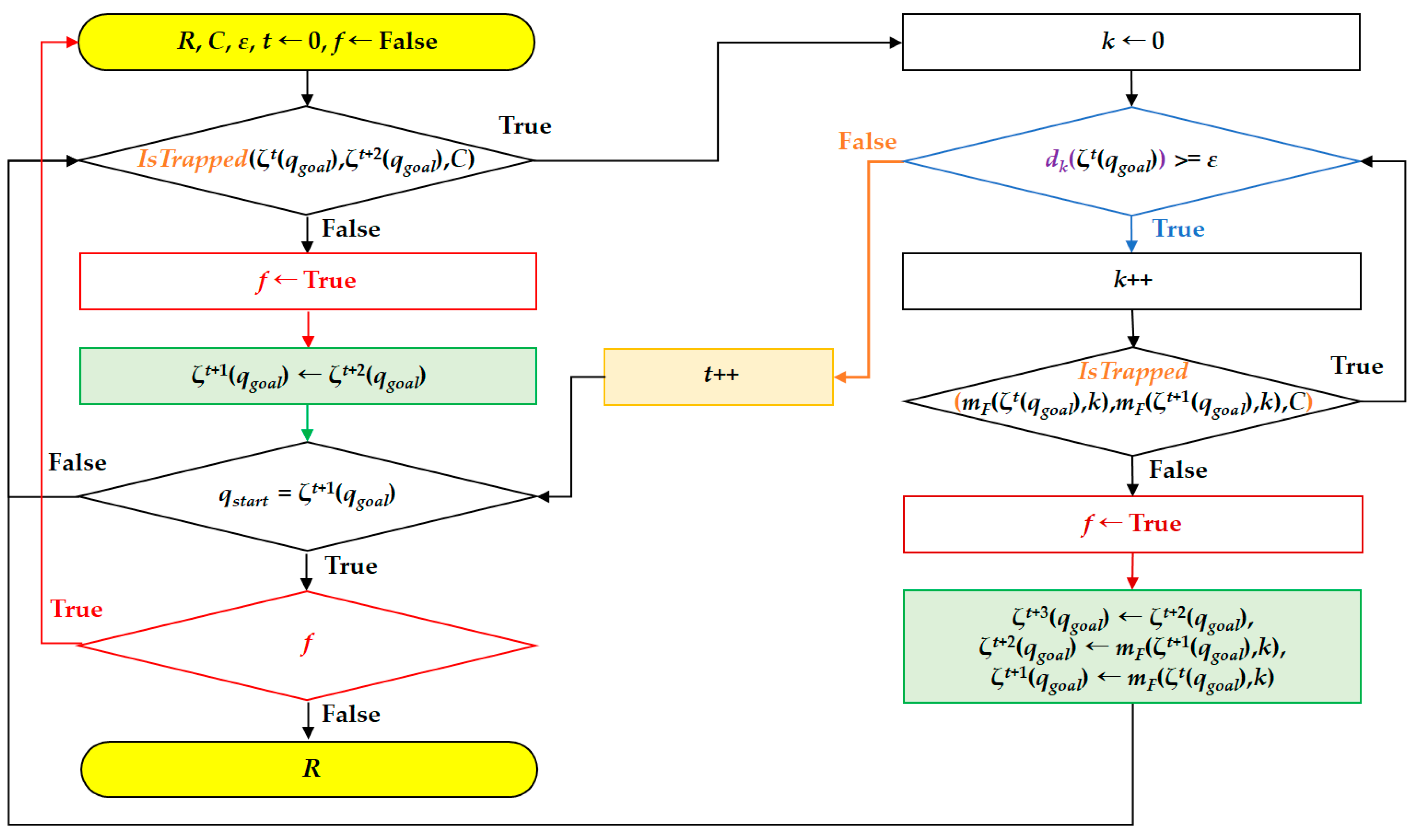
- Check whether the t-th ancestor node and the (t + 2)-th ancestor node of qgoal are collision-free (Here, when t is 0, the 0-th ancestor means itself(qgoal)).
- If the result of Step 1 is not collision-free, compare the dk(ξt(qgoal)) value of the t-th ancestor node of qgoal with ε.
- If dk(ξt(qgoal)) is less than ε, the value of t is incremented by 1, and if the parent node (t + 1) of the t-th ancestor node of qgoal after t is incremented is qstart, the algorithm is stopped (if f is False).
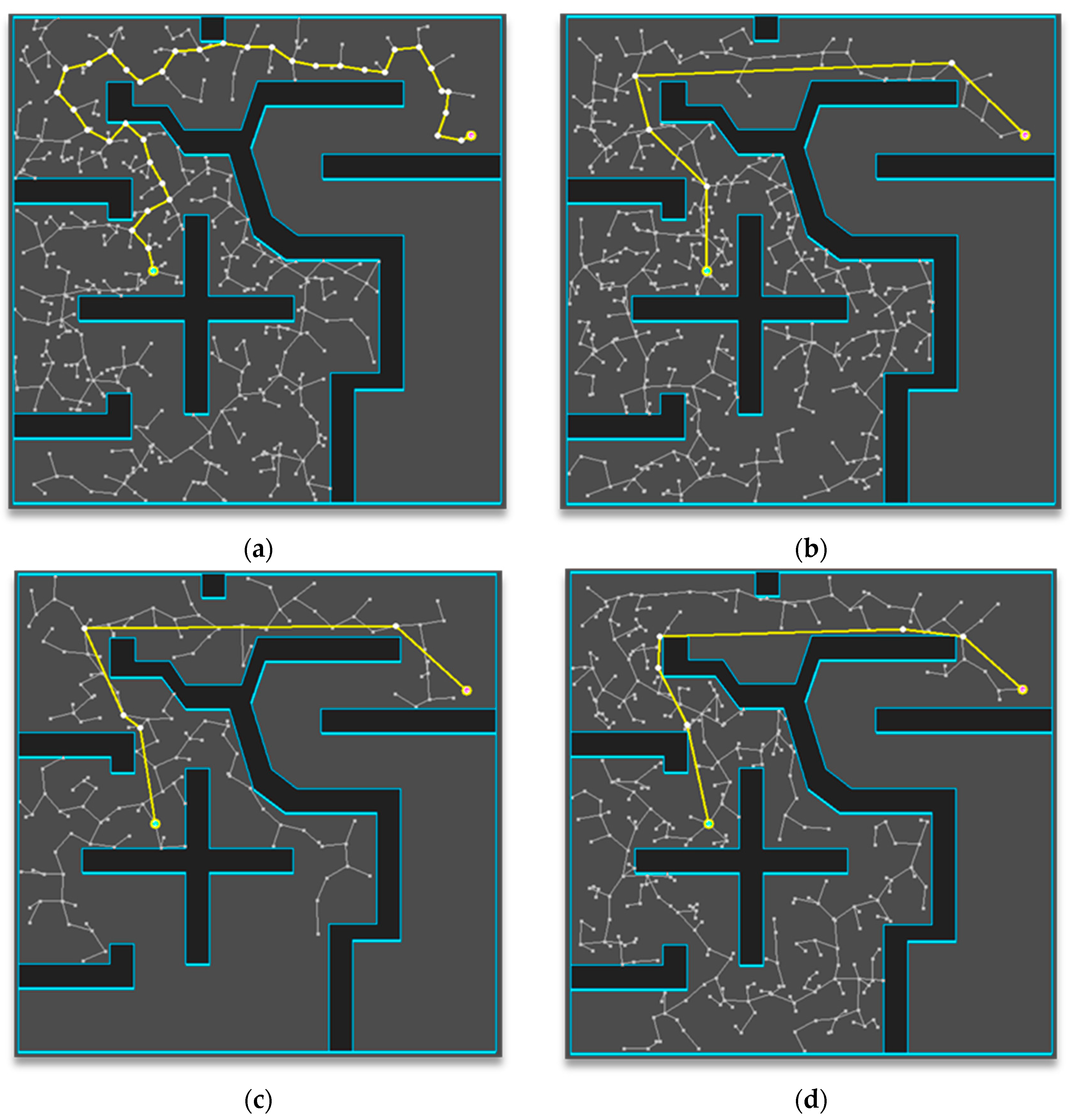
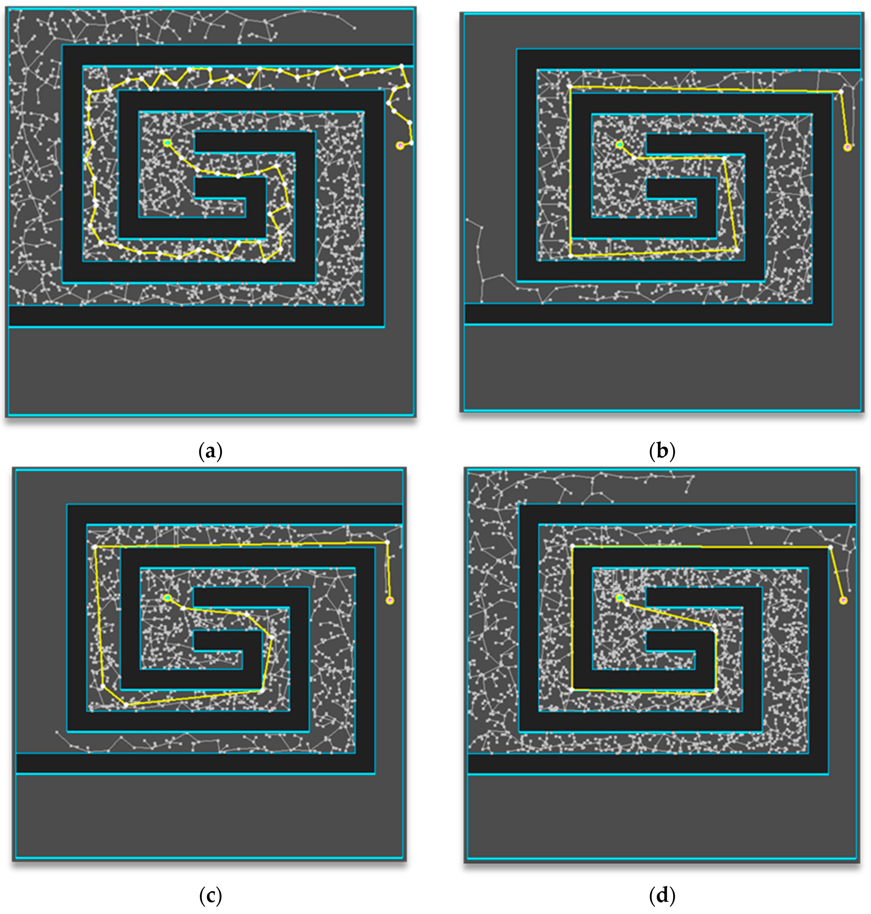
4. Experimental Results
5. Conclusions
Author Contributions
Funding
Institutional Review Board Statement
Informed Consent Statement
Data Availability Statement
Conflicts of Interest
References
- Lindner, L.; Sergiyenko, O.; Moises, R.L.; Ivanov, M.; Julio, C.R.Q.; Daniel, H.B.; Wendy, F.F.; Vera, T.; Fabian, N.M.R.; Mercorelli, P. Machine Vision System Errors for Unmanned Aerial Vehicle Navigation. In Proceedings of the IEEE International Symposium on Industrial Electronics, Edinburgh, UK, 19–21 June 2017; pp. 1615–1620. [Google Scholar]
- Sergiyenko, O.; Wendy, F.F.; Mercorelli, P. Machine Vision and Navigation, 1st ed.; Springer: Cham, Switzerland, 2020. [Google Scholar]
- Abdi, A.; Adhikari, D.; Park, J.H. A novel hybrid path planning method based on q-learning and neural network for robot arm. Appl. Sci. 2021, 11, 6770. [Google Scholar] [CrossRef]
- Schwab, K. The Fourth Industrial Revolution, 1st ed.; Crown Business: New York, NY, USA, 2017. [Google Scholar]
- Wang, X.; Luo, X.; Han, B.; Chen, Y.; Liang, G.; Zheng, K. Collision-free path planning method for robots based on an improved rapidly-exploring random tree algorithm. Appl. Sci. 2020, 10, 1381. [Google Scholar] [CrossRef] [Green Version]
- LaValle, S.M.; Kuffner, J.J., Jr. Randomized kinodynamic planning. Int. J. Robot. Res. 2001, 20, 378–400. [Google Scholar] [CrossRef]
- Kuffner, J.J., Jr.; LaValle, S.M. RRT-Connect: An Efficient Approach to Single-Query Path Planning. In Proceedings of the IEEE International Conference on Robotics and Automation, San Francisco, CA, USA, 24–28 April 2000; Volume 2, pp. 995–1001. [Google Scholar]
- Kang, J.-G.; Lim, D.-W.; Choi, Y.-S.; Jang, W.-J.; Jung, J.-W. Improved RRT-connect algorithm based on triangular inequality for robot path planning. Sensors 2021, 21, 333–364. [Google Scholar] [CrossRef] [PubMed]
- Roy, D. Visibility graph based spatial path planning of robots using configuration space algorithms. Robot. Auton. Syst. 2009, 24, 1–9. [Google Scholar] [CrossRef]
- Katevas, N.I.; Tzafestas, S.G.; Pnevmatikatos, C.G. The approximate cell decomposition with local node refinement global path planning algorithm: Path nodes refinement and curve parametric interpolation. J. Intell. Robot. Syst. 1998, 22, 289–314. [Google Scholar] [CrossRef]
- Warren, C.W. Global Path Planning using Artificial Potential Fields. In Proceedings of the International Conference on Robotics and Automation, Scottsdale, AZ, USA, 14–19 May 1989; Volume 1, pp. 316–321. [Google Scholar]
- LaValle, S.M. Rapidly-Exploring Random Trees: A New Tool for Path Planning; Springer: London, UK, 1998. [Google Scholar]
- Karaman, S.; Frazzoli, E. Sampling based algorithms for optimal motion planning. Int. J. Robot. Res. 2011, 30, 846–894. [Google Scholar] [CrossRef]
- Gammell, J.D.; Srinivasa, S.S.; Barfoot, T.D. Informed RRT*: Optimal Sampling based Path Planning Focused via Direct Sampling of an Admissible Ellipsoidal Heuristic. In Proceedings of the IEEE/RSJ International Conference on Intelligent Robots and Systems, Chicago, IL, USA, 14–18 September 2014; pp. 2997–3004. [Google Scholar]
- Klemm, S.; Oberländer, J.; Hermann, A.; Roennau, A.; Schamm, T.; Zollner, J.M.; Dillmann, R. RRT*-Connect: Faster, Asymptotically Optimal Motion Planning. In Proceedings of the IEEE International Conference on Robotics and Biomimetics, Zhuhai, China, 6–9 December 2015; pp. 1670–1677. [Google Scholar]
- Islam, F.; Nasir, J.; Malik, U.; Ayaz, Y.; Hasan, O. Rrt*-smart: Rapid Convergence Implementation of rrt* towards Optimal Solution. In Proceedings of the IEEE International Conference on Mechatronics and Automation, Chengdu, China, 5–8 August 2012; pp. 1651–1656. [Google Scholar]
- Jeong, I.-B.; Lee, S.-J.; Kim, J.-H. Quick-RRT*: Triangular inequality based implementation of RRT* with improved initial solution and convergence rate. Expert Syst. Appl. 2019, 123, 82–90. [Google Scholar] [CrossRef]
- Jung, J.-W.; So, B.-C.; Kang, J.-G.; Lim, D.-W.; Son, Y. Expanded Douglas–Peucker polygonal approximation and opposite angle based exact cell decomposition for path planning with curvilinear obstacles. Appl. Sci. 2019, 9, 638. [Google Scholar] [CrossRef] [Green Version]
- Jung, J.-W.; So, B.-C.; Kang, J.-G.; Jang, W.-J. Circumscribed Douglas-Peucker Polygonal Approximation for Curvilinear Obstacle Representation. In Proceedings of the IEEE 2019 7th International Conference on Robot Intelligence Technology and Applications (RiTA), Daejeon, Korea, 1–3 November 2019; pp. 237–241. [Google Scholar]
- Kwon, J.; Choi, K. Kinodynamic model identification: A unified geometric approach. IEEE Trans. Robot. 2021, 37, 1100–1114. [Google Scholar] [CrossRef]
- Han, J. Mobile robot path planning with surrounding point set and path improvement. Appl. Soft Comput. 2017, 57, 35–47. [Google Scholar] [CrossRef]


| H/W | Specification |
|---|---|
| CPU | Intel Core i7-6700k 4.00 GHz (8 CPUs) |
| RAM | 32,768 MB (32 GB DDR4) |
| Performance | RRT | Proposed Method (ε: 50 px) | Proposed Method (ε: 30 px) | Proposed Method (ε: 10 px) |
|---|---|---|---|---|
| Path length (px) | 1944 (100%) | 1403 (72%) | 1325 (68%) | 1224 (62%) |
| Planning time (ms) | 697 (100%) | 698 (100%) | 698 (100%) | 698 (100%) |
| Performance | RRT | Proposed Method (ε: 50 px) | Proposed Method (ε: 30 px) | Proposed Method (ε: 10 px) |
|---|---|---|---|---|
| Path length (px) | 986 (100%) | 780 (79%) | 752 (76%) | 730 (74%) |
| Planning time (ms) | 10 (100%) | 10 (100%) | 11 (110%) | 11 (110%) |
| Performance | RRT | Proposed Method (ε: 50 px) | Proposed Method (ε: 30 px) | Proposed Method (ε: 10 px) |
|---|---|---|---|---|
| Path length (px) | 613 (100%) | 535 (87%) | 512 (83%) | 505 (82%) |
| Planning time (ms) | 6 (100%) | 7 (116%) | 8 (133%) | 8 (133%) |
| Performance | RRT | Proposed Method (ε: 50 px) | Proposed Method (ε: 30 px) | Proposed Method (ε: 10 px) |
|---|---|---|---|---|
| Path length (px) | 1536 (100%) | 1284 (83%) | 1261 (82%) | 1190 (77%) |
| Planning time (ms) | 1752 (100%) | 1753 (100%) | 1753 (100%) | 1753 (100%) |
Publisher’s Note: MDPI stays neutral with regard to jurisdictional claims in published maps and institutional affiliations. |
© 2021 by the authors. Licensee MDPI, Basel, Switzerland. This article is an open access article distributed under the terms and conditions of the Creative Commons Attribution (CC BY) license (https://creativecommons.org/licenses/by/4.0/).
Share and Cite
Kang, J.-G.; Choi, Y.-S.; Jung, J.-W. A Method of Enhancing Rapidly-Exploring Random Tree Robot Path Planning Using Midpoint Interpolation. Appl. Sci. 2021, 11, 8483. https://doi.org/10.3390/app11188483
Kang J-G, Choi Y-S, Jung J-W. A Method of Enhancing Rapidly-Exploring Random Tree Robot Path Planning Using Midpoint Interpolation. Applied Sciences. 2021; 11(18):8483. https://doi.org/10.3390/app11188483
Chicago/Turabian StyleKang, Jin-Gu, Yong-Sik Choi, and Jin-Woo Jung. 2021. "A Method of Enhancing Rapidly-Exploring Random Tree Robot Path Planning Using Midpoint Interpolation" Applied Sciences 11, no. 18: 8483. https://doi.org/10.3390/app11188483
APA StyleKang, J.-G., Choi, Y.-S., & Jung, J.-W. (2021). A Method of Enhancing Rapidly-Exploring Random Tree Robot Path Planning Using Midpoint Interpolation. Applied Sciences, 11(18), 8483. https://doi.org/10.3390/app11188483