Abstract
This article examines the mechanisms for cross-border interchange of the regulating reserves (RRs), i.e., the imbalance-netting process (INP) and the cross-border activation of the RRs (CBRR). Both mechanisms are an additional service of frequency restoration reserves in the power system and connect different control areas (CAs) via virtual tie-lines to release RRs and reduce balancing energy. The primary objective of the INP is to net the demand for RRs between the cooperating CAs with different signs of interchange power variation. In contrast, the primary objective of the CBRR is to activate the RRs in the cooperating CAs with matching signs of interchange power variation. In this way, the ancillary services market and the European balancing system should be improved. However, both the INP and CBRR include a frequency term and thus impact the frequency response of the cooperating CAs. Therefore, the impact of the simultaneous operation of the INP and CBRR on the load-frequency control (LFC) and performance is comprehensively evaluated with dynamic simulations of a three-CA testing system, which no previous studies investigated before. In addition, a function for correction power adjustment is proposed to prevent the undesirable simultaneous activation of the INP and CBRR. In this way, area control error (ACE) and scheduled control power are decreased since undesired correction is prevented. The dynamic simulations confirmed that the simultaneous operation of the INP and CBRR reduced the balancing energy and decreased the unintended exchange of energy. Consequently, the LFC and performance were improved in this way. However, the impact of the INP and CBRR on the frequency quality has no unambiguous conclusions.
1. Introduction
1.1. Motivation and Literature Review
The mechanisms for cross-border interchange and activation of the regulating reserves (RRs) are evolving due to the expensive balancing energy, and are included in the European Union’s current regulations [1,2]. They are put in operation in continental Europe by the members of the European network of transmission system operators for electricity (ENTSO-E) [3]. Since the first implementation of the cross-border interchange of the RRs, i.e., the imbalance-netting process (INP), in 2008, the cumulative value of all the netted imbalances amounted to more than €600 million by the third quarter of 2020 [4]. The total monthly volume of netted imbalances for September 2020 was 698.69 GWh, which amounts to €13.38 million. Moreover, the monthly avoided positive and negative RRs activations amount to a minimum of 10% to as much as 85%. The further development of the INP with the functionality of the cross-border activation of the RRs (CBRR), will additionally reduce the activation of the RRs and increase the associated savings.
To avert the activation of the RRs with different signs in the cooperating CAs, and thus reduce the RRs, a grid-control cooperation (GCC) platform was implemented in Germany, where four transmission system operators (TSOs), i.e., 50 Hertz, Amprion, TenneT, and TransnetBW have been collaborating since 2008 [5]. In the following years, many continental European countries joined and the GCC platform developed into the international GCC (IGCC) platform, with the aim to further reduce RRs and increase the reliability of the power system’s operation [6,7,8,9]. Hence, the INP was developed and put in operation, where the cooperating CAs with different signs of power variations can exchange the balancing energy and thus compensate the power variations [10,11]. Therefore, CAs with a surplus of power can exchange with CAs having power shortages [12]. A comparable approach, i.e., area control error (ACE) diversity interchange, was implemented in North America in 1993, but does not consist of actual responses from the control units [13,14,15].
A further reduction of power-system operating costs and increasingly stringent requirements for the quality of the Load-Frequency Control (LFC) defined by the new network codes require further development of the INP with a functionality that will enable CBRR [16]. Therefore, in the first quarter of 2020, the development of the CBRR started that will be put in operation in continental Europe in 2022 [3]. The aim of the development and operation of the CBRR is to improve the ancillary services market and the European balancing system [17]. Similar to the INP, the same control–demand approach and implementation in the control structure will be used for the CBRR. However, the primary objective of the CBRR will be the activation of the RRs in the cooperating CAs and importing into its own CA, thereby reducing the balancing energy [18]. CBRR will only be achievable if the cooperating CAs have matching signs of power deviations. Consequently, CAs with a surplus of power can activate the RRs only in CAs with a surplus of power. Both mechanisms, i.e., INP and CBRR, reduce the balancing energy, while releasing the RRs and, therefore, reducing the associated economic costs. This increases the economic benefits, as the energy exchanged by the INP and activated by the CBRR is additionally financially compensated [19].
A basic schematic diagram of the LFC, INP, and CBRR is given in Figure 1 (left), where the order of the operation is clearly seen. Note here that the correction power is the output of the INP|CBRR block. The main distinction among the INP and the CBRR is in the requirements to compensate for the imbalances among the cooperating CAs. The aim of the INP is to avert the simultaneous activation of RRs with different signs in cooperating CAs, i.e., to net the demand for balancing energy between CAs with different signs of demand power. In contrast, the aim of CBRR is to activate the demand for balancing energy in cooperating CAs with matching signs of demand power. The INP and the CBRR link all the CAs to a joint portal of virtual tie-lines where the INP or CBRR optimization is performed. Note that a virtual tie-line means an additional input of the controllers of the cooperating CAs that has the same effect as a measuring value of a physical interconnector and allows exchange of electric energy between the cooperating CAs [1]. The main objectives of the INP optimization are given in [20,21], whereas the main objectives of the CBRR optimization are given in [22,23].
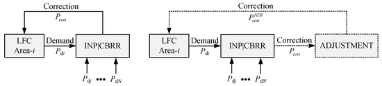
Figure 1.
Schematic diagram of the LFC, INP, CBRR (left) and the function for correction power adjustment (right).
There has been a surge in the application of machine learning and statistical framework to solve similar problems focused in this paper. The authors in [24] explore the influencing factors of consumer purchase intention of cross-border e-commerce based on a wireless network and machine learning in order to provide decision support for the operation of e-commerce and to promote the better development of cross-border e-commerce. Several model-based experimental design techniques have been developed for design in domains with partial available data about the underlying process. The authors in [25] focus on a powerful class of model-based experimental design called the mean objective cost of uncertainty. To achieve a scalable objective-based experimental design, a graph-based mean objective cost of uncertainty with Bayesian optimization framework is proposed. A thorough review of the issues of data localization and data residency is given in [26], in addition to clarifying cross-border data flow restrictions and the impact of cross-border data flows in Asia.
1.2. Contribution and Structure of the Paper
Generally, the INP and the CBRR should have a positive impact on the LFC and performance. However, the quality of the frequency is continually decreasing [27]. Therefore, the impact of the INP and the CBRR on the frequency quality, the LFC, and performance in a three-CA test system was examined separately in [20,22] with dynamic simulations. In [21], the impact of INP on power-system dynamics is shown and an eigenvalue analysis of a two-CA system is conducted. The impact of CBRR on the power-system dynamics is shown in [23], and a modified implementation of the CBRR is proposed that has no impact on the system’s eigendynamics. This article extends these earlier results with an in-depth evaluation of the simultaneous operation of the mechanisms for cross-border interchange and activation of the RRs, which was not studied before. Dynamic simulations are performed for all the cases where the simultaneous operation of the INP and the CBRR is possible. In addition, a function for correction-power adjustment is proposed as one of the contributions of this paper, since small delays in demand power sign change could cause undesired simultaneous activation of the INP and the CBRR. In this way, ACE and scheduled control power are decreased, since udesired correction is prevented. A basic schematic diagram of the LFC, INP, and CBRR and the function for correction power adjustment is given in Figure 1 (right), where the order of operation is clearly seen. Note here that the correction power is the output of the adjustment block. As far as we know, no researchers have examined the impact of the simultaneous operation of the INP and CBRR on the LFC and performance.
This article consists of the following parts: In Section 2, the elemental concepts of the LFC, the INP and the CBRR are described. Simultaneous operation of the INP and the CBRR is also described. Additionally, a function for correction power adjustment is proposed as one of the main contributions of this article, which prevents undesired correction. Section 3 describes indicators for evaluation of the frequency quality, LFC and performance, rate of change of frequency (RoCoF), balancing energy, unintended exchange of energy and energy exchange. In Section 4, a three-CA test system with the INP and the CBRR is described. Two types of test cases were performed with the dynamic simulations, i.e., step change of the load and the random load variation. The primary contribution of this article is given in Section 5, where the impact is given of the simultaneous operation of the INP and the CBRR on the frequency quality, the LFC, and performance. Lastly, Section 6 outlines the main conclusions and outlines future work.
2. LFC, INP, and CBRR
2.1. LFC
An interconnected power system consists of a large number of CAs that are connected via tie-lines. Each individual TSO maintains the frequency of each CA within predefined standard limits and the tie-line power flows with neighboring CAs within prespecified tolerances, which are the main objectives of the LFC [28]. This is generally accomplished by reducing the ACE, which is, for the CA i, defined as
where and denote interchange power variation and frequency deviation, respectively. Note that and denote actual values, while and denote scheduled values. Furthermore, is the frequency-bias coefficient [1]. Note that denotes that the generation is higher than the load; hence, the CA is denoted as “long”. Similarly, a CA is denoted as “short” when .
The basic LFC framework of the CA i is shown in Figure 2, where LPF denotes a low pass filter and SH a sample and hold, with the value of a sampling time s. A negative control-feedback is characterized as −1 gain and PI denotes a proportional-integral controller. Scheduled control power denotes the output of LFC, which is appointed to the participating control units that change the electrical control power appropriately. Neglecting the losses, then is, for the CA i, defined as
where denotes the load-power variation. Note that is well-known as the balancing energy, whereas, instead of LFC reserve, the term RR is generally used.
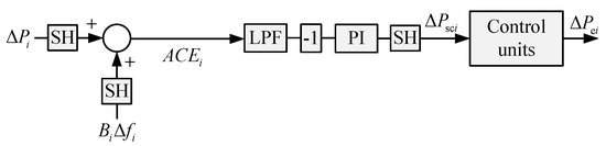
Figure 2.
Schematic block diagram representation of the LFC in the CA i.
2.2. INP
The basic principle of the INP operation and a steady-state correction value calculation with the INP for three CAs is given in [20]. A control–demand concept is used for the INP and a schematic block diagram representation is shown in Figure 3. Commonly, N CAs can be connected via virtual tie-lines, i.e., they can all activate the INP via the interchange factors , , …, marked with the green rectangle. Note that the factor represents the size of the INP interchange of the j-th CA in the i-th CA, where determines that the possible INP interchange is equal to 0%, whereas determines that the possible INP interchange is equal to 100%.
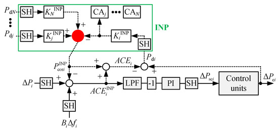
Figure 3.
Schematic block diagram representation of the LFC in the CA i (solid line) with the INP (solid and dotted line).
Moreover, the values of , , …, can be different. The cooperating CAs are connected to the “red” summator, forming virtual tie-lines, as shown in Figure 3. The input variables to the “red” summator are the demand powers of the cooperating CAs, i.e., , , …, . The demand power of the CA i characterizes the maximum interchange power for the CA i among the cooperating CAs and is defined as
according to [3,29].
The power imbalance between generation and load in addition to from the CA i, from CA j, …, from CA N is, for the CA i, defined as
The output variables of the “red” summator are the correction powers of the cooperating CAs, i.e., , , …, , determined with a delay of due to the SH. The correction power of the CA i characterizes the maximum interchange power for the CA i among the cooperating CAs with a different sign of , and is included as
where the terms in brackets denote .
Moreover, only CAs with different signs of demand power, i.e., , can net the demand for balancing energy. If two or more cooperating CAs are “short”, then CBRR is used instead of the INP and vice versa [23]. Therefore, the cooperating CAs must be “short” and “long” in order to net the demand power through the INP. Hence, the balancing energy in CAs that net the balancing energy from the cooperating CAs can be reduced, and simultaneously the RR is released. The , , …, is determined by the INP optimization module, considering numerous target functions, as given in [20].
Considering N CAs, then the is, for the CA i, expressed as
In this way, the correction power of the CA i compensates the load variation that is varied by the frequency variation of the cooperating CAs. From a system point of view, this corresponds to additional frequency-based feedback and cross-couplings with cooperating CAs, which inseparably changes the eigendynamics of the CA i [21].
2.3. CBRR
The basic principle of the CBRR operation and a steady-state correction-value calculation with the CBRR for three CAs is given in [22]. The same control–demand concept is used for the CBRR as is currently used for the INP, and a schematic block diagram representation is shown in Figure 4 [3]. Similar to INP, N CAs can be connected via the virtual tie-lines, i.e., they can all activate the CBRR via the activation factors , , …, marked with the green rectangle. Note that the factor represents the size of the CBRR activation for the CA j in the CA i, where determines that the possible CBRR activation is equal to 0%, whereas determines that the possible CBRR activation is equal to 100%. Moreover, the values of , , …, can be different. The cooperating CAs are connected to the “red” summator, forming virtual tie-lines, as shown in Figure 4.
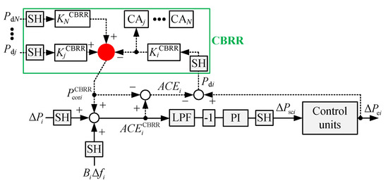
Figure 4.
Schematic block diagram representation of the LFC in the CA i (solid line) with the CBRR (solid and dotted line).
The input variables to the “red” summator are the demand powers of the cooperating CAs, i.e., , , …, . The demand power of the CA i characterizes the maximum activation power for the CA i among the cooperating CAs, defined as (3), according to [3,29].
The power imbalance between generation and load in addition to from the CA i, from the CA j, …, from the CA N is, for the CA i, defined as
The output variables of the “red” summator are the correction powers of the cooperating CAs, i.e., , , …, , determined with a delay of due to the SH. The correction power of the CA i characterizes the maximum activation power for the CA i among the cooperating CAs with matching sign of , and is included as
where the terms in brackets denote .
Moreover, only CAs with matching sign of demand power, i.e., , can activate the demand for balancing energy. If any of the cooperating CAs are “long” and the others are “short”, then INP is used instead of the CBRR and vice versa [21]. Therefore, the cooperating CAs must be either “short” or “long”, depending on whether a positive or negative CBRR is activated. Hence, the balancing energy in CAs that activates the balancing energy in the cooperating CAs can be reduced, and simultaneously the RR is released. The , , …, is determined by the CBRR optimization module, considering numerous target functions, as given in [22].
Considering N CAs, then the is, for the CA i, expressed as
Similar to the INP, the correction power of the CA i compensates the load variation that is varied by the frequency variation of the cooperating CAs. From a system point of view, this corresponds to an additional frequency-based feedback and cross-couplings with cooperating CAs, which inseparably changes the eigendynamics of the CA i [23].
2.4. Simultaneous Operation of the INP and the CBRR
In the cooperating CAs, changes randomly and continuously. Consequently, cases of sign changes can occur, resulting in a continuous switching between the INP and the CBRR, which causes undesirable sign changes. Such a situation might occur when the signs of and are changed with a short time delay. Therefore, a function for adjustment is proposed as one of the contributions of this article.
A schematic block diagram representation for adjustment in relation to of the CA i is shown in Figure 5. The signs of the two successive samples, i.e., and , are compared with the relational operator, whose output is connected to a switch, marked with “c”. Two states are possible, i.e.,
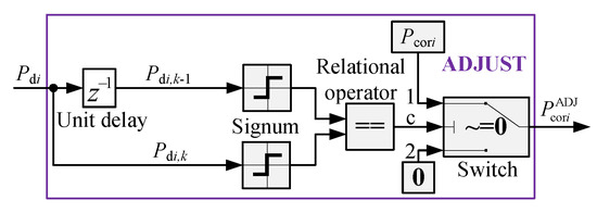
Figure 5.
Schematic block diagram representation for adjustment in the CA i.
- State 1: and
- State 2: .
For State 1, the switch position is “1” and the output variable is . For State 2, the switch position is “2” and the output variable is .
The implementation of the adjustment in the INP and the CBRR framework is shown in Figure 6. The simultaneous operation of the INP and the CBRR, considering the adjustment, can be described using the pseudo-code, as shown in Alogorithm 1.
| Algorithm 1: The code of simultaneous operation of the INP and the CBRR. |
|
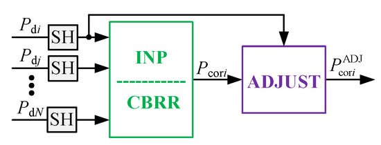
Figure 6.
Schematic block diagram representation for adjustment with the INP and the CBRR in the CA i.
An example of the simultaneous operation of the INP and the CBRR, with and without the adjustment, is shown in Figure 7. The values of the loads were set in such a way that the simultaneous operation of the INP and the CBRR was possible. In the time interval of 80–100 s, the INP operated between CA–CA and CA–CA, whereas the CBRR operated between CA–CA. During this time interval, due to the INP was possible in all three CAs, whereas due to CBRR was possible only in CA and CA. At 100 s, a simultaneous step change of the load in CA and CA was applied, whereas, in CA, it was applied with a delay, i.e., at 100.05 s, as seen at 102 s due to SH with 2 s. Time responses of and at 100 s with one step-size activation of the INP in CA and CA, and the CBRR in CA is clearly seen in Figure 7a (without adjustment). Note that due to CBRR should be zero in CA. Additionally, at 102 s, one step-size activation of the CBRR in CA is also seen. However, in Figure 7b (with adjustment), at 100 s and 102 s, the value of was zero in all CAs. In this way, delayed sign changes have no impact on the switching between the INP and the CBRR. Moreover, the variation is significantly reduced using the proposed adjustment.
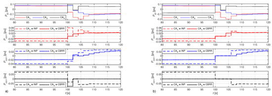
Figure 7.
Time responses of and for a three-CA testing system without adjustment (a) and with adjustment (b), where “w INP” is with the INP and “w CBRR” is with the CBRR.
3. Indicators for Evaluation of LFC, INP, and CBRR Provision
The impact of the simultaneous operation of the INP and CBRR on the frequency quality, the LFC, and performance is evaluated using 15-min averages [1].
3.1. Performance Indicators
Frequency quality is evaluated with the standard deviation of , denoted as . In addition, the LFC and performance is evaluated with the standard deviation of , denoted as [1,30].
3.2. RoCoF
RoCoF is the time derivative of the power system’s frequency, i.e., [31]. The mean value of , denoted as , is evaluated individually for positive and negative values, denoted as and .
3.3. Standard Deviation and Mean Value of RRs
RRs assist in active power balance to correct the imbalance in the transmission grid and lead the power system frequency to the normal frequency range [27]. The standard deviation and mean value of are calculated individually for positive and negative values, denoted as , and , .
3.4. Balancing Energy
The balancing energy enables TSOs to cost-effectively compensate for power and voltage variation in the transmission grid [2]. It is the actual electrical control power that is, for a particular period of time, calculated as . Individual positive and negative values, denoted as and , are calculated.
3.5. Unintended Exchange of Energy
The unintended exchange of energy is determined by the difference between interchange power variation and correction power [2] that is, for a particular period of time, calculated as . Individual positive and negative values, denoted as and , are calculated.
3.6. Energy Exchange
The energy exchange through the INP and CBRR is defined as the actual interchanged or activated power between cooperating CAs [32], that is, for a particular period of time, calculated as . Additionally, positive and negative values are calculated, individually for the INP, denoted as , , and individually for the CBRR, denoted as , .
4. Dynamic Simulations
A three-CA test system was used for the dynamic simulations, where CA–CA and CA–CA were connected by physical tie-lines, whereas CA–CA were not connected with a tie-line. Moreover, all three CAs were connected with virtual tie-lines due to the INP and the CBRR. A Matlab/SIMULINK model was used, where the dynamic simulations were performed with a 50 ms step size.
4.1. Dynamic Model
4.1.1. Structure
The basic schematic block diagram representation of a single CA, characterized with a linearized, low-order, time-invariant model, is shown in Figure 8 and Figure 9 [29,33]. Note that the INP and CBRR implementation is not shown. The generator-load dynamic is described by the rotor inertia and the damping . Moreover, three different types of the turbine-governor systems were considered, i.e., hydraulic, steam reheat, and steam non-reheat. A constant droop characteristic was assumed. In addition, the ramping rate and the participation factors of the control units were also taken into account. The tie-line between the connected CAs is described by the synchronizing coefficient [34]. Furthermore, a 1st-order LPF is modeled by a time constant , while the PI controller is modeled by a gain and a time constant .
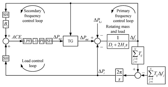
Figure 8.
Schematic block diagram representation of the CA i without the INP and the CBRR.
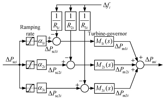
Figure 9.
Schematic block diagram representation of the turbine-governor system with primary frequency control of the CA i.
4.1.2. Parameters
Common parameter values were set for a three-CA test system as given in Table 1 [28,29]. Note that the frequency-bias coefficient was determined as a constant, i.e., . The model parameters were set equally for all three CAs. One cycle of the LFC, INP, and CBRR was incorporated with 2 s.

Table 1.
Parameter values for a three-CA test system.
4.2. Test Cases
The maximum possible compensation with the INP and CBRR was considered. Dynamic simulations were performed so that the loads of individual CAs were altered during the simulation. In addition, two types of test cases were performed, i.e., step change of the load and the random load variation.
Moreover, the inertia time constant , the tie-line parameter , and the droop characteristic have a considerable impact on frequency quality according to [35,36]. Therefore, different values of , , and were used to show the impact of the simultaneous operation of the INP and CBRR on the indicators for evaluation of LFC, INP, and CBRR provision.
4.2.1. Step Change of Load
The values of the loads were set in such a way that the simultaneous operation of the INP and the CBRR was possible. At 0 s, a simultaneous step change of the loads was applied and the magnitudes were set as pu, pu and pu. In addition, at 100 s, the magnitudes were set as pu and pu, whereas, at 100.05 s, the magnitude was set as pu. The resulting load is shown in Figure 10a. Consequently, the INP operated between CA–CA and CA–CA, while the CBRR operated only between CA–CA. Note that this case is used in Section 2.4.
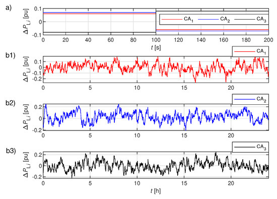
Figure 10.
Step changes of (a) and random variations (b1–b3) for a three CA test system.
4.2.2. Random Load Variation
The random load was modeled as a linear, stochastic, time-invariant, first-order system with two components [37]. A low-frequency component captures the trend changes with a quasi-period of 10–30 min, whereas the residual component captures fluctuations with a quasi-period of several minutes. Measurements of an open-loop ACE in an undisclosed CA were used to determine the model parameters. The resulting normalized load for a three-CA test system with different signs is shown in Figure 10(b1–b3), where the random load was changed every 60 s for 24 h. The statistical parameters of the random loads for all three CAs are given in Table 2, where and denote the meanvalue and the standard deviation of the i-th load, while the correlation between the i-th and j-th loads is denoted as . The correlation is extremely small, which allows both the INP and CBRR to operate simultaneously.
Table 2.
Statistical parameters of random loads.
5. Results
Dynamic simulations with and without the INP and CBRR were performed for a three-CA test system. The impact of the simultaneous operation of the INP and CBRR on the frequency quality, the LFC, and performance was evaluated with the obtained results. Note that the results shown in this section refer to a three-CA test system, whereas the basic principle is applicable to N CAs as shown in Section 2. In addition, the results cannot be generalized to the dynamics of the INP and CBRR.
5.1. Step Change of Load
The time responses to the step change of are shown in Figure 11, Figure 12 and Figure 13. In Figure 11 (left), it is clear that the frequency deviations in all three CAs appeared following a step change of that was applied. After the first step change, and were negative due to the positive step change of , whereas was positive due to the negative step change of . Note that after the second step change, the signs were opposite. The primary frequency control decreased in about 15–25 s after the step change of ; then, LFC decreased slowly. The results show that the impact of the INP and CBRR on is not significant.
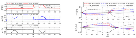
Figure 11.
Time responses of (left) and time responses of and (right) for a three-CA test system, where “wo INP/CBRR” is without and “w INP/CBRR” is with the INP and CBRR.
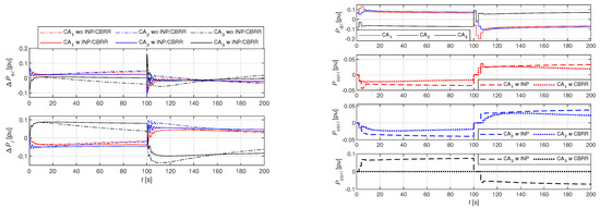
Figure 12.
Time responses of and (left) and time responses of and (right) for a three-CA test system, where “wo INP/CBRR” is without and “w INP/CBRR” is with the INP and CBRR, whereas “w INP” is with the INP and “w CBRR” is with the CBRR.
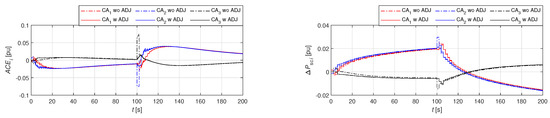
Figure 13.
Time responses of (left) and time responses of (right) for a three-CA test system, where “wo ADJ” is without and “w ADJ” is with the adjustment function.
The impact of the INP and CBRR is shown more obviously in Figure 11 (right) and Figure 12 (left). In all three CAs, the values of , and were decreased with the INP and CBRR. Furthermore, the INP and CBRR clearly increased , due to the increased tie-line power flow between the CAs.
The signs of and are opposite, as shown in Figure 12 (right). A 2 s time delay is seen, due to SH with 2 s. Note that the time responses of and were already described in Section 2.4 and Figure 7b, where the same case was performed.
The time responses and with and without the adjustment function are shown in Figure 13. Without the adjustment, was increased and was undesirably increased, due to switching between the INP and the CBRR, which caused undesirable sign changes. Clearly, in all three CAs, the values of and were decreased with the adjustment. Note that, in Figure 13, the same example is performed as described in Section 4.2.1 and shown in Figure 11 and Figure 12. The difference can be seen because, in Figure 11 and Figure 12, the comparison without and with the INP and CBRR is shown, whereas, in Figure 13, the comparison without and with the adjustment is shown.
5.2. Random Load Variation
Simulations of the simultaneous operation of the INP and CBRR were performed to show the impact of an individual mechanism. The simulations were also performed separately, i.e., operation of only the INP or only the CBRR. The results are given in Table 3, Table 4 and Table 5.
Table 3.
Performance indicators, RoCoF, mean value, and standard deviation of RRs.
Table 4.
Balancing energy and unintended exchange of energy.
Table 5.
Energy exchange.
There are no unambiguous conclusions about the impact of the mechanisms on , and the differences are extremely small, as shown in Table 3. However, both mechanisms reduce , INP slightly more than CBRR. The reduction is most pronounced when both mechanisms operate simultaneously.
Both mechanisms reduce the and , with the reduction being most pronounced when both mechanisms operate simultaneously according to Table 3. However, there are no unambiguous conclusions as to which mechanism reduces and more, and, in most cases, it is the INP.
When both mechanisms operate simultaneously, and are greatly reduced according to Table 3. However, the results of the separate operation of the mechanisms show that the impact of INP is greater than the impact of CBRR. This is expected, as the CBRR only activates the RRs in the cooperating CAs. Moreover, the reduction of and is most noticeable when both mechanisms operate simultaneously. However, the results of the separate operation of the mechanisms show that the impact of the INP is greater than the impact of the CBRR.
The conclusions for and are similar to and according to Table 4, which is expected, as this indicator describes the response of the control units.
When both mechanisms operate simultaneously, and are reduced according to Table 4, except in one case where only was increased, while was reduced considerably. Furthermore, the results of the separate operation of the mechanisms show that the INP almost completely eliminates unintentional deviations, while the impact of the CBRR is not very pronounced.
When both mechanisms operate simultaneously, , , and are slightly reduced compared to separate operation of the INP and CBRR according to Table 5. This is due to the adjustment mechanism, which is only required in the case of simultaneous operation of the INP and CBRR.
Moreover, simulations of the simultaneous operation of the INP and CBRR were performed for different values of , , and . The results are given in Figure 14, Figure 15 and Figure 16.
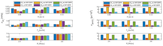
Figure 14.
Average values of (left) and average values of (right) for different values of , and , where “wo INP/CBRR” is without and “w INP/CBRR” is with the INP and CBRR.
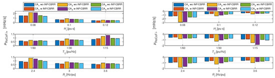
Figure 15.
Average values of (left) and average values of (right) for different values of , and , where “wo INP/CBRR” is without and “w INP/CBRR” is with the INP and CBRR.
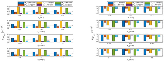
Figure 16.
Average values of (left) and average values of (right) for different values of , and , where “wo INP/CBRR” is without and “w INP/CBRR” is with the INP and CBRR.
There are no unambiguous conclusions about the impact of the mechanisms on , and the differences are extremely small, as shown in Figure 14 (left). In addition, the impact of and is not clear, whereas the increase of results in an increase of . However, both mechanisms significantly reduce , as shown in Figure 14 (right), whereas , and have no impact on .
Generally, both mechanisms reduce the and , as shown in Figure 15. In addition, an increase of and results in a decrease of and , whereas an increase of results in an increase of and . Note that, when pu/Hz, and is increased with the mechanisms.
When both mechanisms operate simultaneously, and are greatly reduced, as shown in Figure 16. However, , and have no impact on and .
6. Conclusions
This article discusses the simultaneous operation of the INP and CBRR, which no previous studies have investigated. Extensive dynamic simulations of a three-CA test system with the simultaneous operation of the INP and CBRR were performed to evaluate their impact on the frequency quality, the LFC, and performance.
The results confirmed the conclusions in [20,21,22,23], where the INP and CBRR were analyzed separately. The results of the step change of load and the random load variation confirmed that the impact of the INP and CBRR on frequency deviations has no unambiguous conclusions. In addition, the impact of inertia and synchronizing coefficient is not clear, whereas the increase of droop characteristic results in an increase of frequency deviations. However, both mechanisms reduce the ACE deviations—the INP slightly more than CBRR. The reduction is most pronounced when both mechanisms operate simultaneously. Moreover, the function for correction power adjustment additionally decreased ACE and scheduled control power, which prevents undesirable switching between the INP and CBRR. Both mechanisms also reduce the RoCoF, and the reduction is most pronounced when both mechanisms operate simultaneously. However, there are no unambiguous conclusions as to which mechanism reduces the RoCoF more, and, in most cases, it is the INP. Increase of inertia and droop characteristic results in a decrease of RoCoF, whereas increase of synchronizing coefficients results in an increase of RoCoF. When both mechanisms operate simultaneously, the scheduled control power is greatly reduced and the impact of the INP is greater than the impact of the CBRR. Similarly, the balancing energy as well as the unintended exchange of energy are greatly reduced when both mechanisms operate simultaneously. However, there is no impact of inertia, synchronizing coefficient, and droop characteristic on scheduled control power. Due to the function for correction power adjustment, which prevents undesirable activation of the INP and CBRR, energy exchange was slightly reduced, as expected. Because of the reduced unintended exchange of energy, beneficial economic consequences can be anticipated when the INP and CBRR operate simultaneously.
One of the tough challenges for all researchers in this domain is the dynamic dimensioning of RRs, considering the INP and CBRR. This article clearly shows that the simultaneous operation of the INP and CBRR reduces the activation of the RRs, which is currently not considered in the reserve dimensioning process.
Author Contributions
Supervision, B.P.; Writing—original draft, M.T.; Writing—review and editing, B.P. All authors have read and agreed to the published version of the manuscript.
Funding
This work was supported by ARRS under Projects P2-0115 and L2-7556.
Institutional Review Board Statement
Not applicable.
Informed Consent Statement
Not applicable.
Data Availability Statement
This study did not report any data.
Conflicts of Interest
The authors declare no conflict of interest.
Abbreviations
The following abbreviations are used in this manuscript:
| RR | Regulating Reserve |
| INP | Imbalance Netting Process |
| CBRR | Cross-Border Activation of the Regulating Reserve |
| CA | Control Area |
| LFC | Load–Frequency Control |
| ACE | Area Control Error |
| ENTSO-E | European Network of Transmission System Operators for Electricity |
| GCC | Grid Control Cooperation |
| TSO | Transmission System Operator |
| IGCC | International Grid Control Cooperation |
| RoCoF | Rate of Change of Frequency |
| LPF | Low Pass Filter |
| SH | Sample and Hold |
| PI | Proportional-Integral |
References
- EUR-Lex. Establishing a Guideline on Electricity Transmission System Operation. Commission Regulation (EU) 2017/1485. Available online: https://eur-lex.europa.eu/eli/reg/2017/1485/oj (accessed on 15 July 2021).
- EUR-Lex. Establishing a Guideline on Electricity Balancing. Commission Regulation (EU) 2017/2195. Available online: https://eur-lex.europa.eu/eli/reg/2017/2195/oj (accessed on 15 July 2021).
- ENTSO-E. Proposal for the Implementation Framework for a European Platform for the Exchange of Balancing Energy from Frequency Restoration Reserves; ENTSO-E: Brussels, Belgium, 2020. [Google Scholar]
- ENTSO-E. IGCC Regular Report on Social Welfare; ENTSO-E: Brussels, Belgium, 2020. [Google Scholar]
- Zolotarev, P.; Gökeler, M.; Kuring, M.; Neumann, H.; Kurscheid, E.M. Grid Control Cooperation—A Framework for Technical and Economical Crossborder Optimization for Load-Frequency Control. In Proceedings of the 44th International Conference on Large High Voltage Electric Systems (Cigre’12), Paris, France, 26–30 August 2012. [Google Scholar]
- Pawalek, A.; Hofmann, L. Utilization of HVDC-Systems in the International Grid Control Cooperation. In Proceedings of the IEEE Milan PowerTech 2019, Milan, Italy, 23–27 June 2019. [Google Scholar]
- Pawalek, A.; Hofmann, L. Comparison of Methods for the Simulation of Dynamic Power Flows in the International Grid Control Cooperation. In Proceedings of the IEEE Electronic Power Grid (eGrid) 2018, Charleston, SC, USA, 12–14 November 2018. [Google Scholar]
- Cronenberg, A.; Sager, N.; Willemsen, S. Integration of France Into the International Grid Control Cooperation. In Proceedings of the IEEE International Energy Conference 2016 (ENERGYCON’16, Leuven, Belgium, 4–8 April 2016. [Google Scholar]
- ENTSO-E. Stakeholder Document for the Principles of IGCC; ENTSO-E: Brussels, Belgium, 2020. [Google Scholar]
- ENTSO-E. Supporting Document for the Network Code on Load-Frequency Control and Reserves; ENTSO-E: Brussels, Belgium, 2013. [Google Scholar]
- Zolotarev, P. Social Welfare of Balancing Markets. In Proceedings of the 14th International Conference on the European Energy Market (EEM) 2017, Dresden, Germany, 6–9 June 2017. [Google Scholar]
- Avramiotis, F.I.; Margelou, S.; Zima, M. Investigations on a Fair TSO-TSO Settlement for the Imbalance Netting Process in European Power System. In Proceedings of the 15th International Conference on the European Energy Market (EEM) 2018, Lodz, Poland, 27–29 June 2018. [Google Scholar]
- Oneal, A.R. A Simple Method for Improving Control Area Performance: Area Control Error (ACE) Diversity Interchange ADI. IEEE Trans. Power Syst. 1995, 10, 1071–1076. [Google Scholar] [CrossRef]
- Zhou, N.; Etingov, P.V.; Makarov, J.V.; Guttromson, R.T.; McManus, B. Improving Area Control Error Diversity Interchange (ADI) Program by Incorporating Congestion Constraints. In Proceedings of the IEEE PES T&D 2010, New Orleans, LA, USA, 19–22 April 2010. [Google Scholar]
- Apostolopoulou, D.; Sauer, P.W.; Dominguez-Garcia, A.D. Balancing Authority Area Coordination with Limited Exchange of Information. In Proceedings of the IEEE Power and Energy Society General Meeting 2015, Denver, CO, USA, 26–30 July 2015. [Google Scholar]
- ENTSO-E. Anual Report 2019 Edition; ENTSO-E: Brussels, Belgium, 2020. [Google Scholar]
- EXPLORE. Target Model for Exchange of Frequency Restoration Reserves. Available online: https://www.tennet.eu/news/detail/explore-target-model-for-exchange-of-frequency-restoration-reserves/ (accessed on 15 July 2021).
- ENTSO-E. Consultation on the Design of the Platform for Automatic Frequency Restoration Reserve (AFRR) of PICASSO Region; ENTSO-E: Brussels, Belgium, 2012. [Google Scholar]
- Gebrekiros, T.Y. Analysis of Integrated Balancing Markets in Northern Europe under Different Market Design Options; NTNU: Trondheim, Norway, 2015. [Google Scholar]
- Topler, M.; Polajžer, B. Impact of Imbalance Netting Cooperation on Frequency Quality and Provision of Load-Frequency Control. In Proceedings of the IEEE International Conference on Environment and Electrical Engineering 2019 and IEEE Industrial and Commercial Power Systems Europe (EEEIC/I&CPS Europe) 2019, Genoa, Italy, 11–14 June 2019. [Google Scholar]
- Topler, M.; Ritonja, J.; Polajžer, B. The Impact of the Imbalance Netting Process on Power System Dynamics. Energies 2019, 12, 4733. [Google Scholar] [CrossRef] [Green Version]
- Topler, M.; Polajžer, B. Evaluation of the Cross-Border Activation of the Regulating Reserve with Dynamic Simulations. In Proceedings of the IEEE International Conference on Environment and Electrical Engineering 2020 and IEEE Industrial and Commercial Power Systems Europe (EEEIC/I&CPS Europe) 2020, Madrid, Spain, 9–12 June 2020. [Google Scholar]
- Topler, M.; Ritonja, J.; Polajžer, B. Improving the Cross-Border Activation of the Regulating Reserve to Enhance the Provision of Load-Frequency Control. IEEE Access 2020, 8, 170696–170712. [Google Scholar] [CrossRef]
- Lu, C.W.; Lin, G.H.; Wu, T.J.; Hu, I.H.; Chang, Y.C. Influencing Factors of Cross-Border E-Commerce Consumer Purchase Intention Based on Wireless Network and Machine Learning. Secur. Commun. Netw. 2021, 2021, 9984213. [Google Scholar] [CrossRef]
- Imani, M.; Ghoreishi, S.F. Graph-Based Bayesian Optimization for Large-Scale Objective-Based Experimental Design. IEEE Trans. Neural Netw. Learn. Syst. 2021, 1–13. [Google Scholar] [CrossRef]
- Meltzer, J.P.; Lovelock, P. Regulating for a Digital Economy—Understanding the Importance of Cross-Border Data Flows in Asia. Glob. Econ. Dev. Work. Pap. 2018, 113, 1–51. [Google Scholar]
- ENTSO-E. Operational Reserve Ad Hoc Team Report; ENTSO-E: Brussels, Belgium, 2012. [Google Scholar]
- Bevrani, H. Robust Power System Frequency Control; Springer: New York, NY, USA, 2009. [Google Scholar]
- Kundur, P. Power System Stability and Control; McGraw-Hill: New York, NY, USA, 1994. [Google Scholar]
- NERC. Frequency Response Standard, Background Document; NERC: Atlanta, GA, USA, 2012. [Google Scholar]
- ENTSO-E. Rate of Change of Frequency (ROCOF) Withstand Capability; ENTSO-E: Brussels, Belgium, 2017. [Google Scholar]
- ACER. Benefits from Balancing Market Integration (Imbalance Netting and Exchange of Balancing Energy); ACER: Ljubljana, Slovenia, 2018. [Google Scholar]
- Anderson, P.M.; Mirheydar, M. A Low-Order System Frequency Response Model. IEEE Trans. Power Syst. 1990, 5, 720–729. [Google Scholar] [CrossRef] [Green Version]
- Elgerd, O.I.; Fosha, C.E. Optimum Mmegawatt-Frequency Control of Multiarea Electric Energy Systems. IEEE Trans. Power App. Syst. 1970, 89, 556–563. [Google Scholar] [CrossRef]
- Vorobev, P.; Greenwood, D.M.; Bell, J.H.; Bialek, J.W.; Taylor, P.C.; Turitsyn, K. Deadbands, Droop, and Inertia Impact on Power System Frequency Distribution. IEEE Trans. Power Syst. 2019, 34, 3098–3108. [Google Scholar] [CrossRef] [Green Version]
- Kundur, P. Definition and Classification of Power System Stability IEEE/CIGRE Joint Task Force on Stability Terms and Definitions. IEEE Trans. Power Syst. 2004, 19, 1387–1401. [Google Scholar]
- Janecek, E.; Cerny, V.; Fialova, A.; Fantík, J. A New Approach to Modelling of Electricity Transmission System Operation. In Proceedings of the IEEE PES Power Systems Conference and Exposition 2006, Atlanta, GA, USA, 29 October–1 November 2006. [Google Scholar]
Publisher’s Note: MDPI stays neutral with regard to jurisdictional claims in published maps and institutional affiliations. |
© 2021 by the authors. Licensee MDPI, Basel, Switzerland. This article is an open access article distributed under the terms and conditions of the Creative Commons Attribution (CC BY) license (https://creativecommons.org/licenses/by/4.0/).