Characterization of Sonic Events Present in Natural-Urban Hybrid Habitats Using UMAP and SEDnet: The Case of the Urban Wetlands

Abstract

We investigated whether the use of technological tools can effectively help in manipulating the increasing volume of audio data available through the use of long field recordings. We also explored whether we can address, by using these recordings and tools, audio data analysis, feature extraction and determine predominant patterns in the data. Similarly, we explored whether we can visualize feature clusters in the data and automatically detect sonic events. Our focus was primarily on enhancing the importance of natural-urban hybrid habitats within cities, which benefit communities in various ways, specifically through the natural soundscapes of these habitats that evoke memories and reinforce a sense of belonging for inhabitants. The loss of sonic heritage can be a precursor to the extinction of biodiversity within these habitats. By quantifying changes in the soundscape of these habitats over long periods of time, we can collect relevant information linked to this eventual loss. In this respect, we developed two approaches. The first was the comparison among habitats that progressively changed from natural to urban. The second was the optimization of the field recordings’ labeling process. This was performed with labels corresponding to the annotations of classes of sonic events and their respective start and end times, including events temporarily superimposed on one another. We compared three habitats over time by using their sonic characteristics collected in field conditions. Comparisons of sonic similarity or dissimilarity among patches were made based on the Jaccard coefficient and uniform manifold approximation and projection (UMAP). Our SEDnet model achieves a F1-score of 0.79 with error rate 0.377 and with the area under PSD-ROC curve of 71.0. In terms of computational efficiency, the model is able to detect sound events from an audio file in a time of 14.49 s. With these results, we confirm the usefulness of the methods used in this work for the process of labeling field recordings.

1. Introduction

Natural-urban hybrid habitats are defined as natural landscapes that are close to an urban context, and they capture the interest of this work. The presence of natural wetlands in cities is vital for many animal species living in them and also offers citizens the possibility of being in touch with nature on a daily basis [1]. Wetlands provide a wide range of benefits to social welfare: (1) climate regulation through the capture of CO${}_2$ emitted into the atmosphere [2]; (2) flood protection during heavy rains [3]; (3) water quality improvement (acting as filters by absorbing large amounts of nutrients and a variety of chemical contaminants) [4,5]; (4) a habitat for preserving insects, plants and animal life [6]; and (5) cultural services and non-use values [7], such as educational and artistic values [8], recreation and reflection, aesthetic experiences [9], a sense of place [10,11] and, particularly, sonic heritage [12].

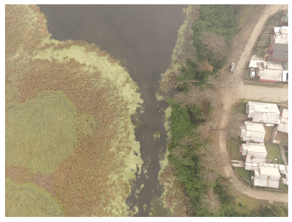
While urban wetlands provide the above mentioned benefits, concerns about their degradation have increased in recent years [13]. Most of the literature on urban wetlands assumes that they are interrelated patches [14] of a landscape mosaic [15] rather than islands separated by inhospitable habitats [16] (see Figure 1).

It is clear from recent research that urban wetlands are under threat as a consequence of the intensification of anthropogenic activities associated with increases in population [17]. As a result of this phenomenon, wetland landscapes are changing, with green spaces becoming increasingly urbanized. These changes in habitats can produce competition and predation in certain species, which would modify the characteristics of the landscape [18]. This produces an increase in the fragmentation of these interrelated pieces of a mosaic and, as a result, diverse proximal patches and the loss of a connection among them, simultaneously affecting the biodiversity contained [19].

In order to deal with this issue, we took inspiration Tobler’s first law of geography [20], which states that if a given patch of the original mosaic, owing to anthropogenic activities, is divided into two patches, then both patches should be related.

This law predicts that regardless of the distance between the two patches, they will always have interrelationships with each other, but the smaller the geographical distance between the patches, the stronger these interrelationships [21].

Thus, our first hypothesis is that the smaller the distances among urban wetlands, the more similar their acoustic environments will be. Under this hypothetical viewpoint, urban wetlands can be considered as habitat patches of a landscape mosaic that have been fractured over time because of the urban growth of the city. By investigating the temporal evolution of sonic events present in each patch, one can estimate the effects of the temporal changes in the city on these patches. In this context, in order to measure whether the sonic structures are similar among habitats, we use only acoustic features, and hence we require a substantial amount of labeled sonic data extracted from field recordings carried out in each patch. However, the process of labeling these recordings is costly and time consuming. The second hypothesis is that the use of supervised deep learning methods such as SEDnet can be faster and more time efficient than the traditional process of labeling field recordings carried out in these natural-urban habitats. We analyze interactions and temporal similarities among the habitat patches depending on their closeness in the space of the city and synchronism of acoustic events throughout the day.

Valdivia is a medium-sized city in the south of Chile that is rich in urban wetlands [22]. We selected and compared three natural–urban habitats of the city. These patches have undergone intervention at varying scales over time, which may be due to their different geographical locations within the city and their interactions with the anthropogenic components of the urbanized landscape [23]. We employ, for feature visualization purposes, the uniform manifold approximation and projection (UMAP) unsupervised algorithm [24] to represent, in a 2D space, the similarity and separability of the acoustic features of the urban wetlands. Moreover, we adopt the concept of Jaccard’s similarity, grouping the patches in pairs to evaluate their synchronicity over time and quantify sonic similarities between the habitats. We highlight that among social species, individuals living in the same group might have synchronized activities (e.g., movements and vocalizations) [25]. We believe that the method used here can be adapted and extended to any kind of environment of biological interest.

In order to optimize the labeling task, we tackle the challenge of complementing manual annotations with the use of new methods that automatically detect sound events of interest [26,27]. We assume here that the samples of sonic events have class labels with no errors annotated by the experts. Unfortunately, manual annotation is an error-prone task, especially when the number of hours of the recording to be labeled increases. However, long field recordings are needed to understand the effects that the changes occurring in the city have on these habitat patches [28]. We employ machine-learning and data-mining methods as they are two of the most accepted techniques for this purpose nowadays [29]. We create a manually labeled dataset consisting of common and characteristic sonic events present in the three natural–urban wetlands. In order to validate our second hypothesis, we used this dataset to train a deep learning model based on SEDnet [30] to automatically detect sonic events in these patches and evaluate its performance using an independent test set.

The paper is organized as follows. Section 2 describes related works in the field of sonic event characterization, with a focus on natural-urban habitats and on the use of technological tools to manipulate field recordings in long periods. In Section 3, we describe the three habitats studied, as well as the materials and methods used in the context of the research. The experimental results are presented in Section 4. In Section 5, we discuss the research findings, and in Section 6 we provide conclusions and possible future developments of the work.

2. Background and Related Works

Farina et al. (2021) [31] specified that, in recent decades, sound has been recognized as a universal semiotic vehicle that represents an indicator of ecological structures and that is a relevant tool for describing how animal dynamics and ecosystem processes are affected by human activities.

Farina [32] compiled the fundamentals of various processes in animal communication, in community aggregation and in long-term monitoring, as well as in several processes of interest in ecology, providing space for soundscape ecology and ecoacoustics.

Bradfer-Lawrence et al. (2019) [33] explored various ecoacoustic practices, such as the use of various acoustic indices that reflect different attributes of the soundscape and recording collection methods.

Gan et al. (2020) [34] explored the problem of acoustic recognition of two frog species by using long-term field recordings and machine-learning methods. Acoustic data were extracted from 48 h of field recordings under different weather conditions. These data were used to conduct experiments and to assess recognition performance. The labeling task of frog chorusing was performed manually by trained ecologists who proposed, as features, spectral acoustic indices extracted from the recordings’ spectrograms.

For recognition experiments, they used the following as supervised learning algorithms: support vector machine (SVM), k-nearest neighbors (kNN) and random forest. The best score reported was 82.9% of accuracy obtained with the SVM classifier and combinations of synthetic and real-life data.

Mehdizadeh et al. (2021) [35] report that there is evidence that certain species at birth produce calls that are important in mother-child communication that are characterized mostly by calls of low frequency, multi-harmonic and with specific temporal pattern. As they grow, these songs grow shorter in duration and their frequency rises. This is an evidence that indicates that the sonic characteristics of these species change with age, and that this should, therefore, be taken into consideration.

De Oliveira et al. (2020) [36] developed a task for the acoustic recognition of birds and specified that this requires large amounts of audio recordings in order to be used by machine-learning methods. In this case, the main problem is the processing time. They addressed this issue by evaluating the applicability of three data reduction methods. Their hypothesis was based on the notion that data reduction could highlight the central characteristics of features without the loss of recognition accuracy. The investigated methods were random sampling, uniform sampling and piecewise aggregate approximation. They used Mel-frequency cepstral coefficients (MFCC) as features and hidden Markov models (HMM) as learning algorithms. The most advantageous method reported was uniform sampling, with a 99.6% relative reduction in training time.

Sophiya and Jothilakshmi (2018) [37] addressed the classification of 15 different acoustic scenes, both outdoors and indoors, and the problem of expensive computation time in the training stage. They used the architecture of a deep multilayer perceptron as the baseline system. For the experiments, they employed the datasets from the 2017 IEEE AASP Challenge on the Detection and Classification of Acoustic Scenes and Events (DCASE) and 40 mbe (log of Mel-scale frequency energy) features as feature vectors, extracted every 40 ms of frame length and overlapped at 50%. They divided the dataset into three parts for training (60%), validation (20%) and testing (20%), and each trained model was evaluated by using a four-fold cross-validation approach. They reported an averaged overall result of 74% accuracy for the baseline system and a computation time of 20 min 40 s. When they used the Apache Spark MLlib platform along with the baseline system, they achieved 79% accuracy and a computation time of 0 min 55 s.

Knight et al. (2020) [38] addressed the problem of how to predict whether the detection of a recognizer of two bird species that uses machine-learning methods is a true or false positive. By means of employing audio recordings, they used HMM, convolutional neural networks (CNN), and a training method with denominated boosted regression trees (BRT). The results for the two species studied (Chordeiles minor and Seiurus aurocapilla) showed a reduction in the number of detections that required validation by 75.7% and 42.9%, respectively, while retaining at least 98% of the true-positive detections.

Lostanlen et al. (2018) [39] developed a method for modeling acoustic scenes and for measuring the similarity between them. They used the bag-of-frame (BoF) approach for acoustic similarity, which models an audio recording using the statistics of short-term audio attributes based on MFCC. The performance of the BoF approach is successful for characterizing sound scenes with little variability in audio content but cannot accurately capture scenes with superimposed sound events.

In the context of Chile, urban wetlands have a highly significant value for the inhabitants of the city of Valdivia, which have been increasing over time. Over the past two decades, wetlands legislation and policy have evolved significantly. There has been debate surrounding this issue, with citizen participation of the main social and environmental scientists from Chilean universities, different social actors, policy makers and private sector representatives [40]. These recent events demonstrate that the majority of the local community are willing to protect, use and plan these natural-urban habitats. In 2020, the Chilean Parliament approved a law that aims to protect urban wetlands declared by the Ministry of the Environment of Chile [41].

As highlighted by Mansell [42] (2018), this recognised high social value of urban wetlands enables inhabitants to gain a sense of belonging to nature even in their sonic dimension. Mansell notes that our sonic environment is an essential element of the cultural politics and of the urban identity that can help us to rethink how the natural-urban habitats are conceptualized and developed.

In addition, as was noted by Yelmi [12] (2016), for any urban identity, the sonic values that define the city connect people to their culture and their lands and relate them to their geographical location, climate and the everyday routine of a community or a region. For this reason, Yelmi states methods for protecting the characteristic sounds of everyday life of the city (e.g., wind, water and market noises) from a sonic viewpoint in order to strengthen the cultural memory of the city.

However, it is very important to understand that despite government efforts, debates and citizen participation, urban wetlands are ecosystems that are extreme fragile and particularly vulnerable to urban changes and anthropogenic pressure, as was mentioned by Chatterjee and Bhattacharyya (2021) [43] (2021). The authors note that severe habitat fragmentations are primary drivers of biodiversity loss, and that mammals are particularly vulnerable to this fragmentation.

3. Materials and Methods

The work presented here is part of a research project supported by the National Fund for Scientific and Technological Development, FONDECYT, Chile (2019–2021), conducted to implement a interdisciplinary platform in order to enhance the sonic heritage of the urban wetlands of Valdivia, Chile, from the application of a new sonic time-lapse method [44,45].

Periodic 5 minute stereo field recordings were carried out every hour during a year in the three wetlands of the city of Valdivia. The collected recordings include a variety of sound sources that characterize the acoustic scene of the wetlands, which can be divided into three categories: anthropophony (human-produced sounds), geophony (geophysical sounds) and biophony (biological sounds).

We believe that the research presented here provides a preliminary analysis of the collected data due to the fact that we only considered ten days of recordings in each habitat, equivalent to 720 processed audio files, representing approximately 3% of a complete dataset. It is worth mentioning that one year of field recordings results in 26,280 generated audio files that need to be processed and analyzed efficiently. The analyzed dataset with annotations comprises more than two days and twelve hours of samples of sonic events with class labels.

3.1. Field Recordings for Long Periods and Sonic Events of Reference

An inherent characteristic of these three natural–urban habitats studied is that the sonic events collected came from distinct sound sources.

These common and characteristic acoustic events are present in each habitat. We analyzed a set of five events of reference ($E_r$) that comprise the vocalizations of birds, amphibians and dogs without distinction of subspecies or ages in addition to rain and mechanical engines, including both fixed sources (e.g., woodchippers commonly present in certain areas of the city) and mobile sources (e.g., motorcycles, cars, buses and trucks). With this acoustic framework in mind, we carried out synchronous field recordings using three water-proof programmable sound recorders, Song Meter SM4 Wildlife Acoustics [46], mounted on tree trunks approximately at 3.0 m above ground level. These robust and affordable digital recorders collected audio samples during the first five minutes of each hour for 5 days (27–31 October 2019) and then 5 more days at a following date (6–10 January 2020). Synchronous recordings of sonic event data in the three wetlands were made by using two omnidirectional microphones per set of equipment at a sampling frequency of 44,100 samples per second so that any sonic event data of up to 22.050 kHz could be distinguished. Each audio recording was saved as a 16-bit PCM uncompressed .wav file.

3.2. Habitat Descriptions

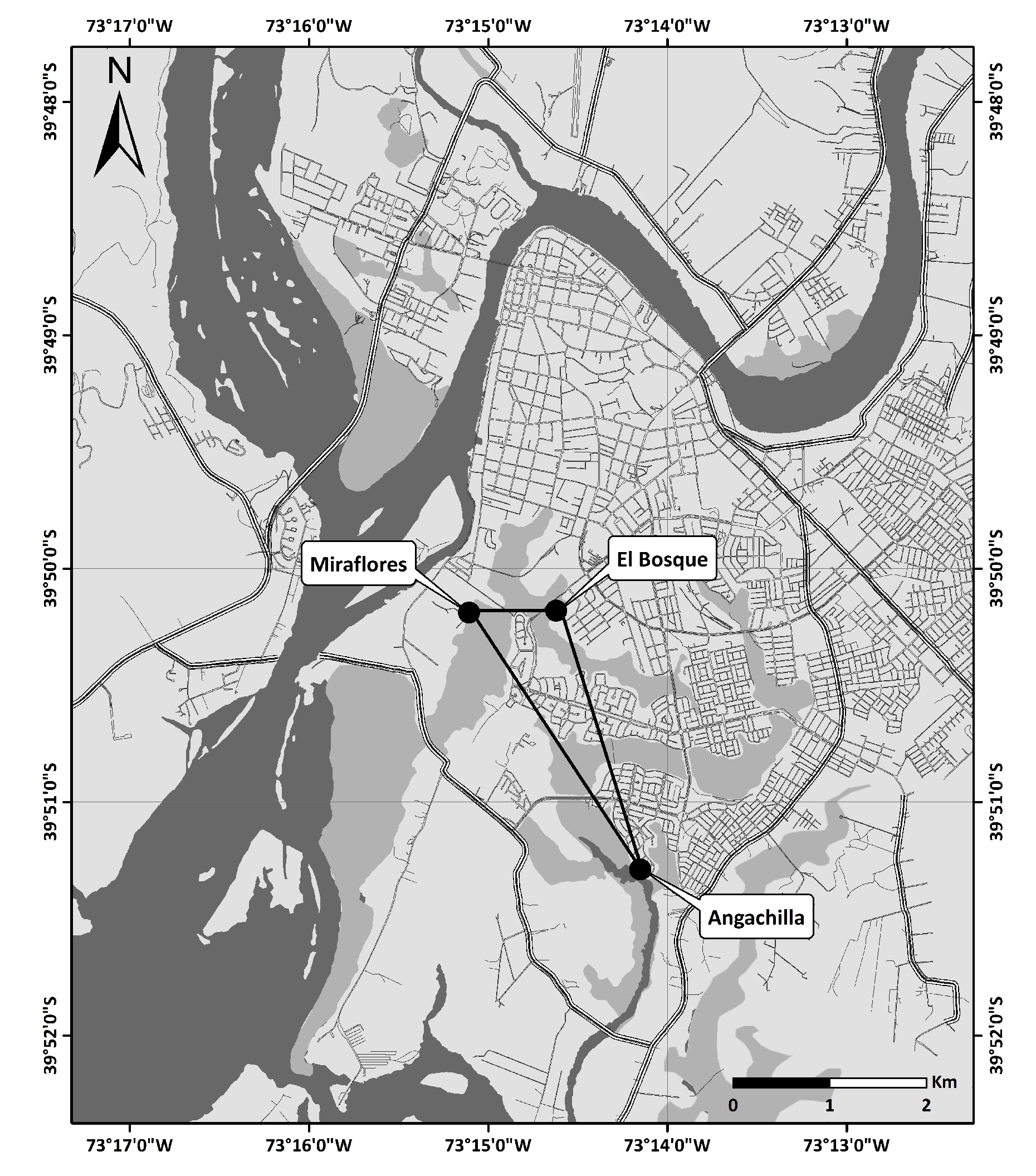
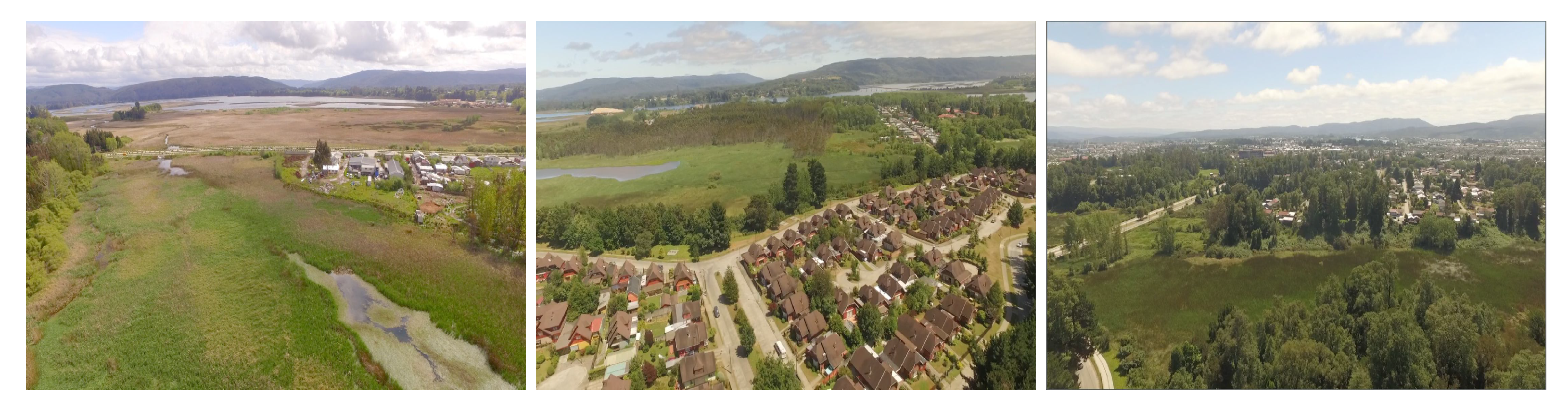
Valdivia is a southern city of Chile ($39°{48}^{\prime }{00}^{″}\mathrm{S}73°{14}^{\prime }{00}^{″}\mathrm{W}$) located at a confluence of several rivers, one of which, the Cruces River, is within one of the aquatic biodiversity hotspots of the world [47]. Within the boundaries of the city are 77 urban wetlands [22]. The experimental part of the study took place at three urban wetlands in Valdivia: Angachilla ($39°{51}^{\prime }{24}^{″}\mathrm{S}73°{14}^{\prime }{06}^{″}\mathrm{W}$), Miraflores ($39°{50}^{\prime }{22}^{″}\mathrm{S}73°{15}^{\prime }{07}^{″}\mathrm{W}$) and El Bosque ($39°{50}^{\prime }{21}^{\prime }\mathrm{S}73°{14}^{\prime }{37}^{″}\mathrm{W}$) (see Figure 2 and Figure 3). The approximate geographical distances between the recording positions at Angachilla–Miraflores, Angachilla–El Bosque and Miraflores–El Bosque were 2300 m, 2040 m and 700 m, respectively. The Angachilla wetland is the farthest habitat from the city center. It is located in an urban sector with patches of green areas with the presence of small mammals as well as a significant number of birds of prey. On the other hand, the Miraflores wetland is located in a mixed residential and industrial area with factories surrounding it, such as shipyards and woodchippers that operate continuously 24 h a day for seven days a week. This wetland has muddy substrates, is characterized by its calm waters, is protected from the wind and has urban swamps grazed by local horses. The El Bosque wetland is located in an urban residential area of the city with a prevalence of hospital, school and commercial activities. It is characterized by the surrounding shallow waters, with little streams and shadowy areas given its high vegetation, which constitute an excellent refuge habitat, especially for groups of birds. Some bird species found in these natural-urban habitats are pequén (Athene cunicularia), chucao (Scelorchilus rubecula) and cisne de cuello negro (Cygnus melancoryphus). Moreover, the amphibian species present include sapo (Eupsophus roseus) and sapito de anteojos (Batrachyla taeniata). Based on the literature, the fauna records in the urban wetlands of Valdivia show that the wetland fauna is dominated by 71 species of birds (76% of the total), as well as 5 species of amphibians (5% of the total). The rest of the fauna diversity comprises mammals, fish, crustaceans and small reptiles. The urban areas of the city of Valdivia are characterized by dwellings with concrete walls, where loud, continuous sounds of low frequency are dominant components of the urban landscape [23,48].

3.3. Manual Labeling Process

The total amount of field recordings used to carry out our analysis of sonic events consists of 720 audio files that are two-channeled (stereo) and stored in .wav format. These audio files were recorded at three natural-urban habitats synchronously. Before the feature extraction stage, we carried out manual labeling to obtain a ground truth for the sonic event analysis. We annotated the reference events ($E_r$) in each of the audio files, which are characteristic and common at each habitat. As a result, our ground truth contains information on the audio file name, wetland name, day and hour of the recording, start and end times of each event and the names of the events in that time interval. In our auditory analysis of the recordings, we found some time intervals containing more than one sonic event; we call this situation a multi-event. Meanwhile, we refer to the presence of a single event as simply a single event. Both multi-events and single-events constitute the classes ($C_p$) that we may find during the auditory analysis of the audio files. The ground truth data cover an approximated total period of two days and twelve hours of annotations.

3.4. Sonic Feature Extraction Process

The feature extraction stage is based on the log energies of Mel-frequency scale triangular filter bank outputs (mbe from here on) [30] that use a short-time Fourier transform process to estimate time-varying spectra. The number of Mel filters used was 40 bands on each audio channel. During this process, each input audio recording was divided into overlapping sequential sample windows called frames. In this study, a fixed window size of 2048 samples was used, which is 46 ms, considering our sampling frequency of 44,100 samples per second and an overlap between subsequent windows of 50%. This provides a reasonable commitment between time and frequency resolution. Prior to the Fourier transform, we used a Hanning window function in each frame. The magnitude spectrum of the Fourier transform was estimated frame by frame using 2048 frequency bins (21.5 Hz per bin).

3.5. Dataset Analysis

After an audio file has been partitioned into small time frames, we establish a criterion for unifying the durations of sonic events to create a class label ($L_c$) and associate it with each frame, taking as reference the known ground truth data [30]. The advantage for using mbe acoustic features to train a classifier and visualize features within a 2D space is that we also used them to analyze temporal changes in quantities and distributions of classes, considering both single events and multi-events throughout the day. 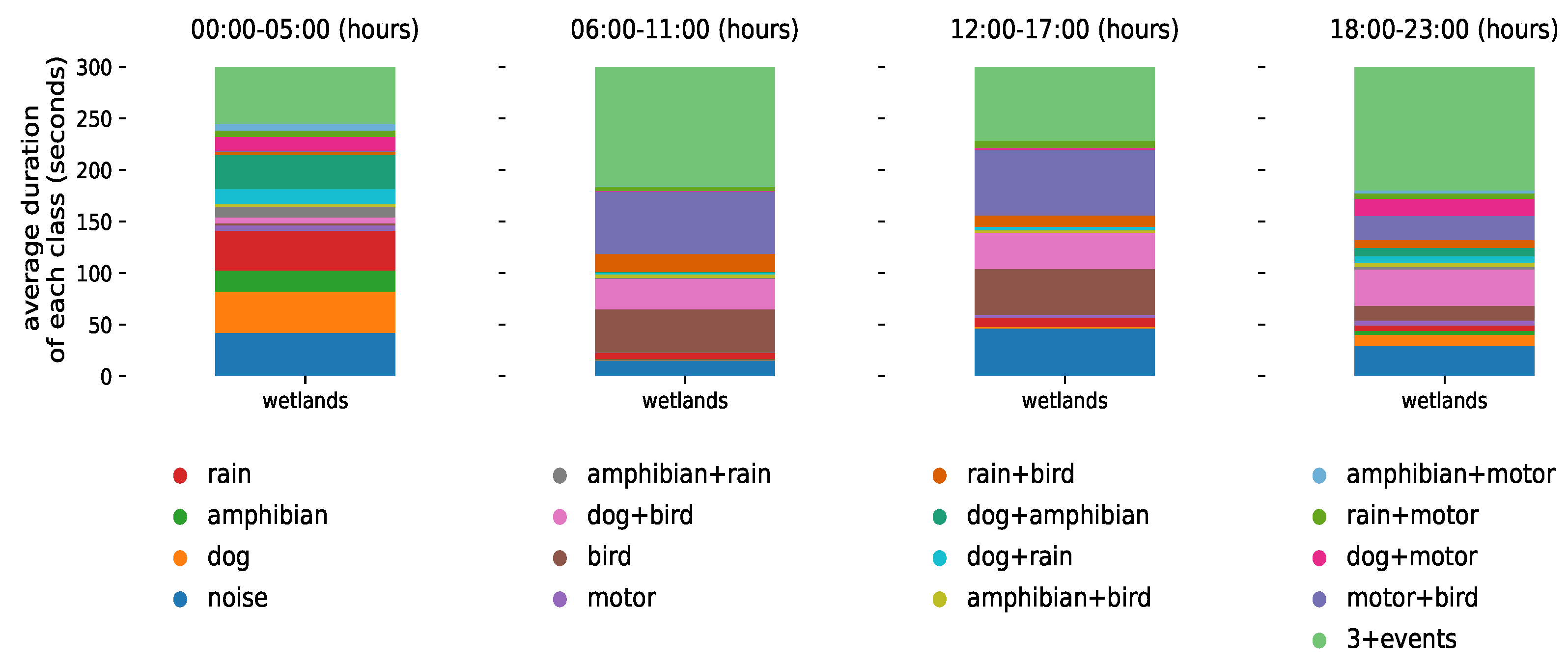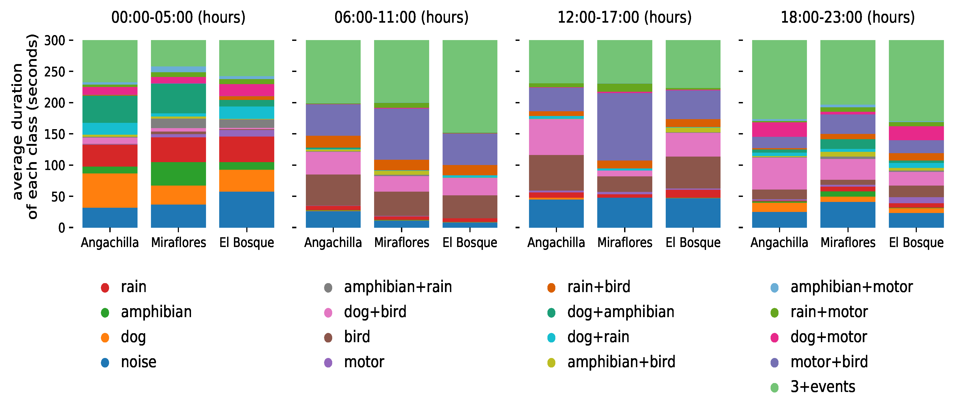Figure 4 shows a summary of the global temporal evolution of the classes (and their quantities) of all the datasets collected at the three urban wetlands during the ten-day experiment. Each day was divided into four six hour periods, with an early morning peak between 00:00 a.m. and 05:00 a.m., a morning peak between 06:00 a.m. and 11:00 a.m., an evening peak between 12:00 p.m. and 17:00 p.m. and a nighttime peak between 18:00 p.m. and 23:00 p.m. We expressed the average duration of each class and all its possible combinations in seconds. The value of 300 s on the ordinate axis corresponds to the period of 5 min during which the audio samples were recorded per hour.

3.6. Data Visualization Using UMAP

Before training the neural network classifier, we propose to visually inspect the data using unsupervised learning techniques. The objective is to explore and assess if the different sonic events, as characterized by their mbe features, form groups or clusters. As these data might be too complex for linear methods, we propose to perform dimensionality reduction using the Uniform Manifold Approximation and Projection (UMAP) [24], a state of the art algorithm that non-linearly projects the data to a low dimensional manifold, aiming to preserve the topology of the original space.

The UMAP algorithm is applied on 1,950,438 frames from 720 recordings belonging to single-events. The input dimensionality is 40, which corresponds to the number of mel filter banks (two channels). The output dimensionality is set to 2. Due to the large volume of data, we consider the high-performance and GPU-ready implementation of the UMAP algorithm found in the cuML library [49]. The hyperparameters for obtaining the low-dimensional embeddings are as follows:

• Size of the local neighborhood: 35;
• Effective minimum distance between embedded points: 0.1;
• Effective scale of embedded points: 1;
• Initialization: spectral embedding.

These hyperparameters were obtained by qualitative assessment of the resulting visualizations.

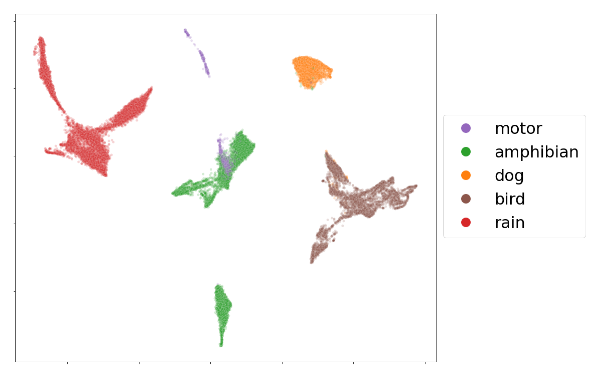
As an example, we present a visualization of the mbe features of seven audio recordings (33,431 frames) containing single events in Figure 5. From the embedding, it is clear that the five labeled classes, birds, amphibians, dogs, rain and motors, can be easily separated by their mbe features. We note, however, that most of the time, the audio data coming from the field recordings show the presence of multi-events, which makes class separation extremely difficult for an event detection model in a machine-learning perspective.

3.7. Sonic Comparisons among Habitats

We compared the three habitat patches, which over the years have changed from natural to urban habitats, by using their sonic characteristics collected in field conditions. Comparisons of similarity or dissimilarity among the patches were based on the Jaccard coefficient (J). These comparisons were carried out in pairs: Angachilla–Miraflores, Angachilla–El Bosque and Miraflores–El Bosque. For the analysis of sonic similarity or dissimilarity between the pairs, we considered Tobler’s first law of geography and supposed that, under this law, two habitat patches might share similarities with each other and that the smaller the geographical distance between the patches, the stronger these similarities. In our analysis, we assumed that we have five reference sonic events, which are denoted as $E_r=\{E_1,\dots ,E_5\}$ with $n_E=5$ as the number of events. We defined the total number of potential classes as $n_C=2^{n_E}$ arising from the different combinations of events, including both the absence of events (noise) as well as single events and multi-events. For a particular day, under field conditions we have 24 audio files (one for each hour of the day). In a frame-by-frame analysis, we associated one of the classes $C_j\in \{C_1,C_2,\dots ,C_{n_C}\}$ where $1\le j\le n_C$ to a particular frame (i-th frame) with its label $L_i$ with $1\le i\le n_L$, where $n_L$ is the number of frames in which all the audio files were divided. In order to compare the temporal variation between a pair of habitats A and B in the particular hour of a determined day, we selected from A its i-th frame, $A_i$, and from B its i-th frame, $B_i$, where i is a frame synchrony index (that is, the index i varies in such a way that $A_i$ and $B_i$ move forward together). We defined $\mathrm{J}(C^A,C^B)$ as the Jaccard similarity coefficient for a particular frame.

$$\mathrm{J}(C^A,C^B)=\frac{|C^A\cap C^B|}{|C^A\cup C^B|}$$

(1)

We interpreted the Jaccard coefficient as the intersection of the classes $C^A$ and $C^B$ divided by their union—that is, the more the two classes overlap when superimposed on each other, the larger their intersection and the greater the similarity coefficient. The values of J can range between 0 and 1, where a result of 1 means that the two classes are identical and a result 0 means that the classes have no sonic characteristics in common. We calculated the average Jaccard coefficient by hour, summing up the coefficients frame by frame and dividing by $n_L$:

$$\overline{\mathrm{J}}=\frac{{\sum }_{i=1}^{n_L}\mathrm{J}(C_i^A,C_i^B)}{n_L}$$

(2)

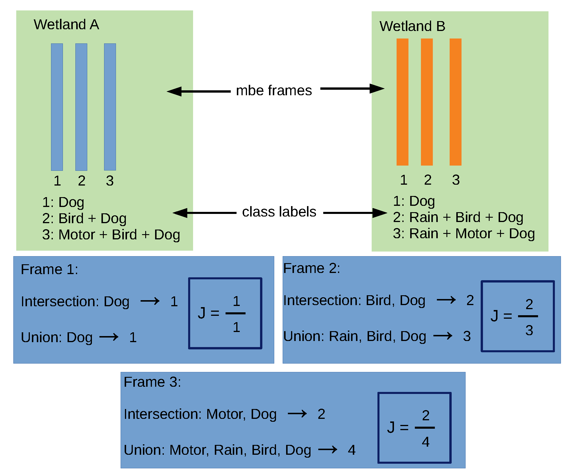
where $C_i^A$ is the class label for the i-th frame of wetland A and $C_i^B$ is the class label for the i-th frame of wetland B. We explained the computation process of J in a frame-by-frame manner, as seen in Figure 6. We take two wetlands, A and B, and use three of their synchronous time frames, where each frame has an associated class label. For instance, the second frames in A and B have, as an intersection, two events in common (Bird and Dog), while they have, as a union, three events detected in the time frame (Rain, Bird and Dog). As a result, J is obtained as the ratio between the intersection and the union of the class labels for the frame.

3.8. Neural Network Model for Sonic Event Detection (SED)

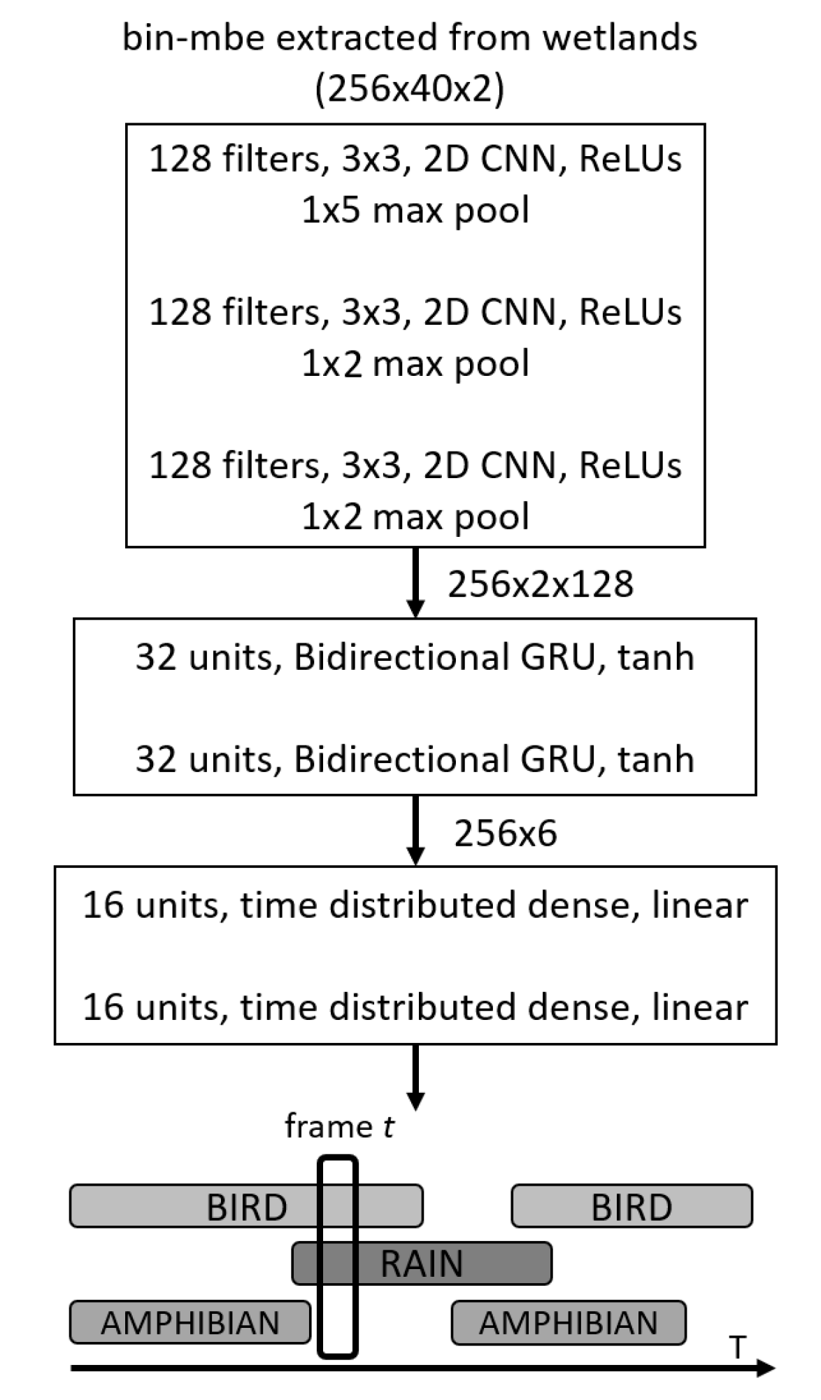
Figure 7 shows a schematic summary of the neural network model in operation. This architecture, which is commonly referred to in the literature as SEDnet [30], is a particular type of convolutional recurrent neural network. Our motivation to use this system is based on the fact that it has shown high capability for recognizing sonic events on real-life datasets [50], achieving first place (minimum error rate) in the third task of the DCASE Challenge 2017 [51]. For this particular case, the input to the model is the set of mbe features previously extracted from the audio files in the feature extraction stage. In what follows, we explain the different processing stages of the model.

The initial stage is composed of three convolutional layers which perform two tasks. First, shift-invariant features can be extracted layer by layer at different time scales; secondly, this can reduce the feature dimensionality, reducing training time and testing time. The Rectified Linear Unit (ReLU) is used as the activation function in these layers. The feature maps are then fed into a second stage based on a special type of recurrent layer called the bidirectional gated recurrent units (GRUs) [52]. The tanh activation function is used in these layers. The GRU layers specialize in learning temporal structures contained in the features and are easier to train in comparison to other recurrent layers. These recurrent units also help predict the onsets and offsets of sonic events. The output of the recurrent layers is proceeded by two fully connected (FC) dense layers with sigmoidal activations in order to predict the presence the probability of sonic events. The output of the SEDnet corresponds to the predicted event probabilities over time, i.e., a vector with one element per event and where all elements are in the range of $[0,1]$. In order to define whether an event is present or absent, we defined a threshold known as the operating point, which indicates that if the event is present its probability is above this point, otherwise the event is absent.

Field recordings containing 720 audio files were used as dataset during the SEDnet training procedure. The dataset was shuffled and splitted in order to assess the generalization capacity of the sonic event detector model. We implemented a four-fold cross validation procedure, where in each fold 75% of the data were used for training and 25% for testing. Moreover, a third of the training data in each fold was selected randomly as validation data. The model is trained by minimizing a distance between a reference and the sonic event predictions. In this case we consider the binary cross-entropy loss as an objective function to detect both sonic single events and multi-events that are commonly present in natural-urban habitats. The adaptive moment estimation (ADAM) method [53] with mini-batches of the data is used to minimize the loss and update the weights of the SEDnet model. The maximum number of training epochs, i.e., complete iterations through the entire training dataset, is set to 500. Early stopping is considered to avoid overfitting. The training stops if the F1-score in the validation set does not improve for 50 epochs. To In order to address overfitting, the dropout regularization technique [54] is also considered. Dropout switches off a random subset of the FC layers neurons every epoch during training. This avoids co-adaptation and improves generalization.

The detection performance of SEDnet depends on several hyperparameters. The following combinations of the most sensible hyperparameters are evaluated using a grid search strategy:

• The size of the minibatch: varied from 32 to 256 in steps of multiples of 2;
• The length of the sequence: varied from 64 to 1024 in steps of multiples of 2;
• The initial learning rate: vested values are 0.0001, 0.001 and 0.01;
• The dropout rate: varied from 0.25 to 0.75 in steps of 0.05.

The best hyperparameter combination is found by maximizing the average F1-score for the four-fold validation partitions.

Metrics and Performance

In order to quantify the performance of the SEDnet model, we used two groups of metrics. The first group includes the multi-event F1-score and the error rate, as proposed in [30]. The F1-score is defined as follows:

$$\mathrm{F}1-\mathrm{score}=\frac{{\sum }_{k=1}^{K}2·TP\left(k\right)}{{\sum }_{k=1}^{K}2·TP\left(k\right)+FP\left(k\right)+FN\left(k\right)}$$

(3)

where

• $TP\left(k\right)$, the number of true positives for event k, is the number of frames in which sound event k is present in both the groundtruth and in the predictions;
• $FP\left(k\right)$, the number of false positives for event k, is the number of frames in which sound event k is present in the predictions but not in the groundtruth;
• $FN\left(k\right)$, the number of false negatives for event k, is the number of frames in which sound event k is present in the groundtruth but not in the predictions.

Note that in order to compute these metrics, we need to set a threshold for the detection probabilities given by the SEDnet model. This threshold can be set in a event by event basis, i.e., we can adjust the sensitivity of different sound events independently. Unless specified, this threshold is set to $0.5$ for all events. After thresholding, a binary decision representing either the presence or the absence of the sound event is obtained. From these metrics, we can write the multi-event error rate as follows:

$$error\_rate=\frac{{\sum }_{k=1}^{K}min(FP\left(k\right),FN\left(k\right))+max(0,FN\left(k\right)-FP\left(k\right))+max(0,FP\left(k\right)-FN\left(k\right))}{{\sum }_{k=1}^{K}N\left(k\right)}$$

(4)

where $N\left(k\right)$ is the total number of labels of event k present in groundtruth. A good model should have an error rate close to zero and a F1-score close to one.

The second group of metrics includes the True Positive Ratio ($TPR\left(k\right)$), False Positive Rate ($FPR\left(k\right)$) and Cross-Trigger Rate ($CTR\left(k\right)$) for sound event k, as proposed in [55]. These are defined as $TPR\left(k\right)=TP\left(k\right)/N\left(k\right)$, $FPR=FP\left(k\right)/T_N$ and $CTR=CT\left(k\right)/\sum {\Delta }_L$, respectively. The cross-triggers ($CT$) represent a subset of the $FP$ that match another labeled event of the set of events, and $\sum {\Delta }_L$ is the sum of the differences between offset and onset for each label. From these equations, we computed the effective $FPR$ ($eFPR$) that combines $FPR$ and $CTR$ through the parameter ${\alpha }_{\mathrm{CT}}$:

$$\mathrm{eFPR}\left(k\right)=\left\{x\right|x=FPR\left(k\right)+{\alpha }_{\mathrm{CT}}·\mathrm{mean}\left({\mathrm{CTR}\left(\mathrm{k}\right)}_e\right),\forall e\in E_r\}$$

(5)

where $E_r$ is the set of sound events of reference. In this case we use ${\alpha }_{\mathrm{CT}}=1$ to consider all the CTR values.

The $TPR\left(k\right)$, $FPR\left(k\right)$ and $eFPR\left(k\right)$ can be computed for a set of thresholds $\tau =[0,\dots ,1]$ or operating points to obtain the polyphonic sound detection receiver operating characteristic (PSD-ROC) curves. These curves provide a more complete comparison between different models and also allow us to search for the optimal threshold values for the different events. Finally, we also consider the area under the PSD-ROC curves as a summary statistic of the performance of the model under all possible operating points.

4. Results

The results of the calculations of the hourly average values of $\overline{\mathrm{J}}$ for the ten days of activity in the experiments are summarized in

Table 1. Temporal variations of average Jaccard coefficient $\overline{\mathrm{J}}$ in four periods of six hours.

Jaccard Coefficients	Periods (hours)				Mean
between Wetlands	00:00–05:00	06:00–11:00	12:00–17:00	18:00–23:00
Angachilla–Miraflores	0.415	0.526	0.428	0.402	0.443
Angachilla–El Bosque	0.392	0.531	0.459	0.449	0.458
Miraflores–El Bosque	0.359	0.556	0.443	0.414	0.443

. We present these temporal variations in four six-hour periods, with an early morning peak between 00:00 a.m. and 05:00 a.m., a morning peak between 06:00 a.m. and 11:00 a.m., an evening peak between 12:00 p.m. and 17:00 p.m. and a nighttime peak between 18:00 p.m. and 23:00 p.m.

Additionally, we disaggregated the temporal evolution of the classes by its geographical origin (wetland), as seen in Figure 8. We maintain the same time-periods used in Table 1 to facilitate comparison of the information among the habitats.

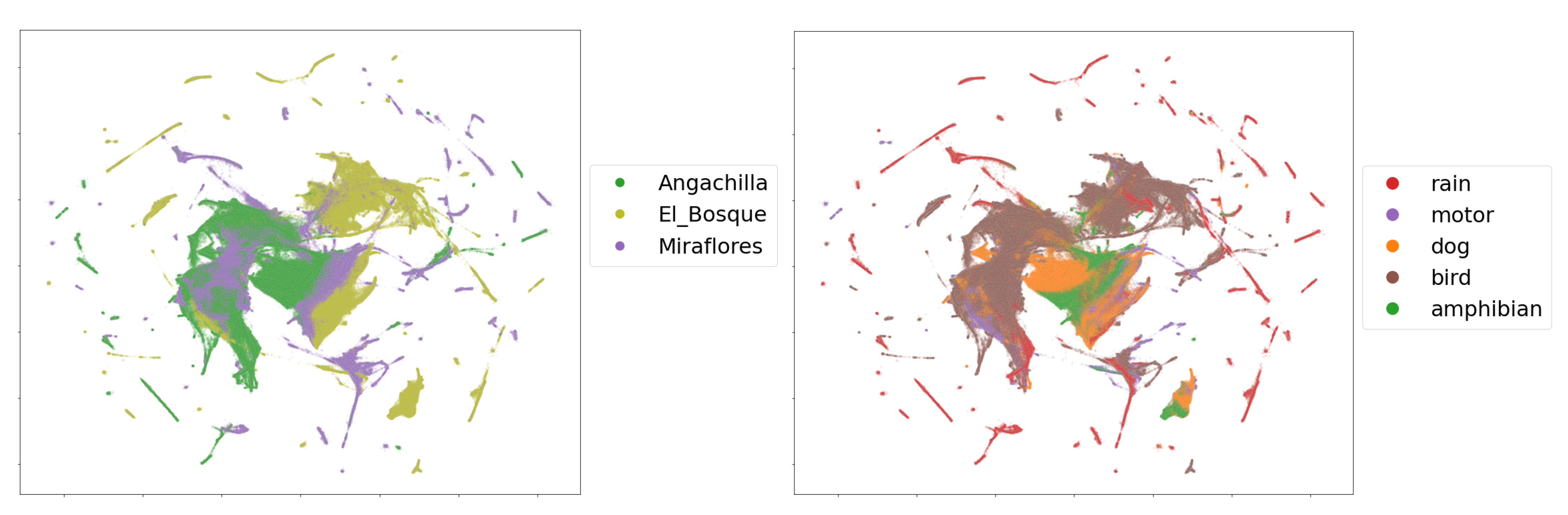
Figure 9 shows the two dimensional embedding obtained by applying the procedure described in Section 3.6 over the complete dataset of mbe features. The upper and lower subfigures show the embeddings of the frames colored by their geographical origin and labeled single-event, respectively.

The quality of the experimental results of SEDnet is assessed by using the F1-score and error rate metrics. We conducted exhaustive experiments to compare the detection performance of SEDnet by tuning the hyper-parameters and the number of audio files for training. The results presented here are based on the best set of hyper-parameters, which are as follows:

• Learning rate: 0.001;
• Batch size: 32;
• Dropout probability: 0.5;
• Sequence length: 1024 frames.

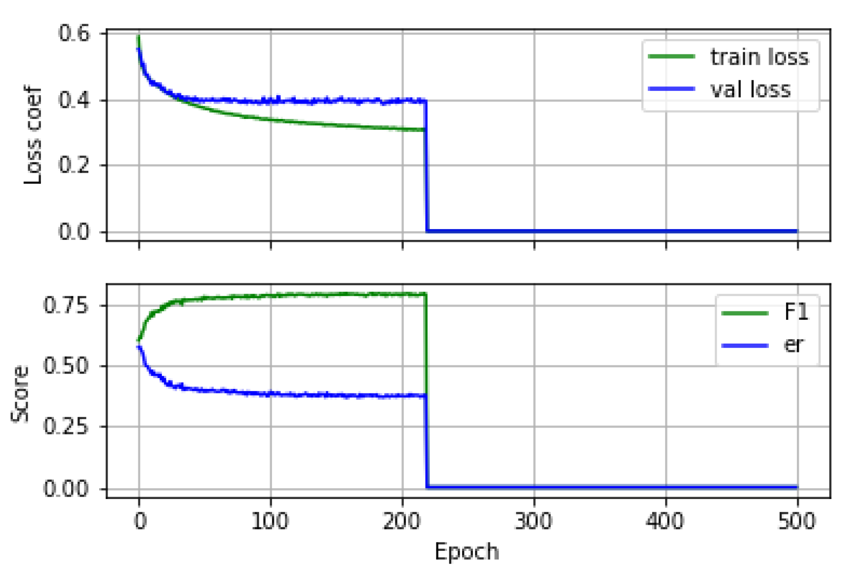
An example of the training and validation learning curves and the evolution of the performance metrics during training is shown in Figure 10.

The average values of the F1-score and the error rate obtained from the four folds are provided in

Table 2. Average F1-score and average error rate for the best fold and average labeling time.

SEDnet	F1-Score	Error Rate
Average 4-folds	0.784	0.391
Best fold	0.790	0.377

. In addition, for the best fold (according to training), we show the F1-score and error rate.

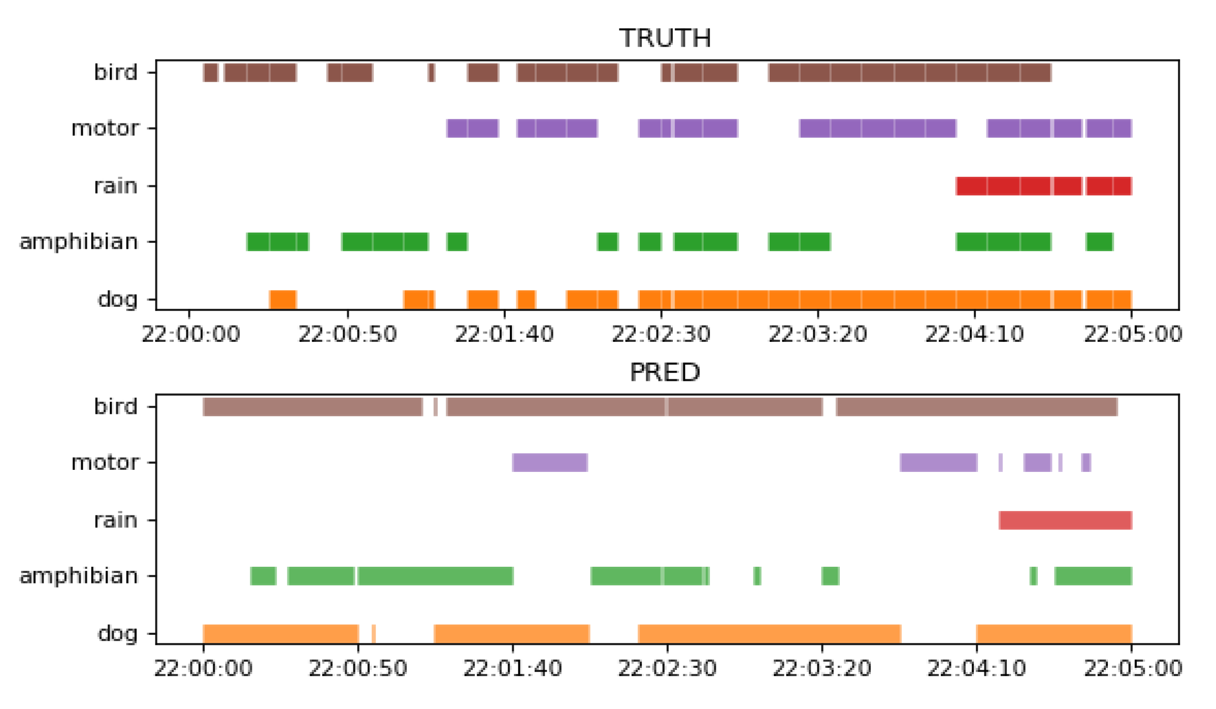
Figure 11 shows a comparison between the ground truth of a 5 min recording from the test set and the corresponding SEDnet prediction using the best model from Table 2.

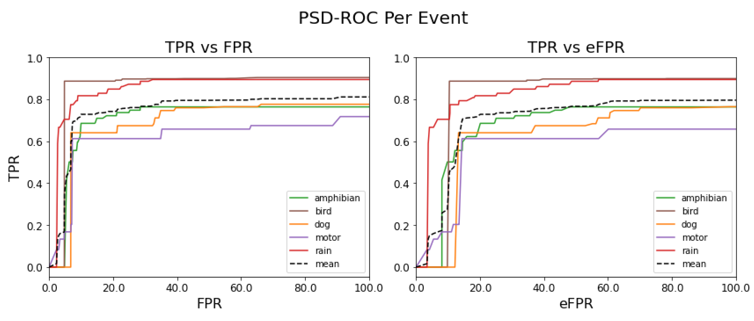
All the results presented so far were obtained with the default threshold of $0.5$. We explore the performance as a function of the threshold or operating points using PSD-ROC curves. Figure 12 shows the PSD-ROC curves per sound event (colored solid lines) and the average PSD-ROC curve (black dashed line).

Table 3. Areas under the five PSD-ROC curves and the mean value.

AUC	Amphibian	Bird	Dog	Motor	Rain	Mean
TPR vs. FPR	67.800	82.345	65.837	59.112	81.847	71.000
TPR vs. eFPR	65.368	78.875	69.186	55.282	80.864	68.000

shows the areas under these PSD-ROC curves.

Finally, in terms of computational efficiency, the best model was able to detect sound events from an audio file (5 min) in a time of 14.49 ± 0.17 s.

5. Discussion

The Jaccard similarity analysis found differences among the three habitat patches, which also differ in the temporal evolution of their sonic classes arising from the different combinations of natural and urban events in the early morning, morning, evening and at night. These differences partially support our first hypothesis. As observed in Table 1, only the habitat patches Miraflores and El Bosque, which possess the shortest geographical distance (700 m), had a reasonable similarity in their sonic characteristics composition (average coefficient of Jaccard = 0.556). This occurred particularly in the morning period between 06:00 a.m. and 11:00 a.m., reaching the highest degree of agreement with Tobler’s law, confirming our first hypothesis. However, in contrast with Tobler’s prediction, in the early morning between 00:00 and 05:00 a.m., these two habitat patches exhibited the lowest similarity degree (average coefficient of Jaccard = 0.359), refuting our first hypothesis in this period. The low similarity between Miraflores and El Bosque in the early morning would suggest a temporal variation in the composition, structure and diversity of the sonic classes. The Miraflores and El Bosque wetlands had a high presence of sonic single events in the early morning, as observed in Figure 8. Unlike the morning period in these same habitats, the presence of the motor and bird single events, as well as that of the sonic class containing the (motor + bird) combination, was almost negligible in the early morning.

This led us to concentrate on the other classes that were still present in the early morning, especially the behavior of the amphibian class. This class is clearly present as a single event, and its combination with the dog event is also present in an important sonic class, (dog + amphibian). As can be observed in Figure 8, 62% of the amphibian class occurred in the Miraflores wetland, while only 20% occurred in the El Bosque wetland. The sonic class that contains the (dog + amphibian) combination occurred predominantly in the Miraflores wetland, with a presence of 47º%, while in the El Bosque wetland it occurred at a rate of only 10%. Similarly, the noise class with unidentifiable sounds or no events was more predominant in the El Bosque wetland (46%) than in the Miraflores wetland (29%). The greater presence of the amphibian event in the Miraflores wetland compared with the El Bosque wetland, together with a higher percentage of the noise class in the El Bosque wetland in comparison to the Miraflores wetland, would justify the lowest Jaccard coefficient in the early morning.

Our findings lead us to reconsider our first hypothesis in light of the temporal variation of sonic classes. As one of our objectives was to highlight the importance of both the green habitats within the city and the sonic events in these habitats, we analyzed the temporal associations between single events and multi-events, both in quantities and in distributions of classes throughout the day, without distinguishing among the habitats. Figure 4 shows the complexity of these sonic associations collected in the three habitat patches during the ten days of activity covered by the experiments. We found that the early morning period between 00:00 and 05:00 a.m. had the greatest presence of single events, especially rain, amphibians and dogs. Similarly, the greatest presence of multi-events, three or more events simultaneously, occurred in the morning (06:00–11:00 h) and at night (18:00–23:00 h), and these were evident over many seconds. This could be due to the presence of periodic anthropogenic activities, which are associated with the start and end of daily activities in the city, especially daily peaks of intense vehicle traffic, that have an impact on the natural habitat. When we disaggregated the data of the global temporal evolution of classes at the level of wetlands, as observed in Figure 8, we found, through the single-event analysis at the early morning period, that the Miraflores wetland had a greater number of sonic events of amphibians (62%) compared with the El Bosque wetland (20%), as explained above, as well as in comparison to the Angachilla wetland (18%).

Similarly, the Angachilla wetland had a greater number of sonic events of dogs (46%) compared with the El Bosque (29%) and Miraflores (25%) wetlands. Furthermore, as observed in Figure 8, one of the most apparent sonic changes observed in these three habitats between the early morning and morning periods was associated with sonic patterns of amphibian and bird activity. Specifically, the amphibian event occurred earlier at dawn compared with the bird event, which leads us to define the offset time of the daily sonic activity of amphibians in the early morning and the onset time of the daily activity of birds in the morning. Our results are consistent with those of previous studies that demonstrate that birds avoid exposure to artificial light at night [56], and that the calling activity of amphibians starts around sunset and extends to the first half of the night [57].

One non-natural sonic event that was present in the data shown in Figure 8 was the motor event along with its combination with the bird event, which is represented in the (motor + bird) sonic class. As observed in the figure and for the three habitats, in the morning (06:00–11:00 a.m.), 45% of the (motor + bird) class occurred in the Miraflores wetland, 28% in the El Bosque wetland and 27% in the Angachilla wetland. Meanwhile, in the evening (12:00–17:00 p.m.), 56% of the (motor + bird) class occurred in the Miraflores wetland, 24% in the El Bosque wetland and 20% in the Angachilla wetland. Finally, at night (18:00–23:00 p.m.), 45% of the (motor + bird) class occurred in the Miraflores wetland, 29% in the El Bosque wetland and 26% in the Angachilla wetland. We deduce from this result that the habitat patch associated with the greatest presence of the (motor + bird) class was the Miraflores wetland in the morning, in the evening and at night. Our result is consistent with the location of this habitat in an urban mixed residential and industrial area, with the presence of factories working around it that operate 24 h a day, indicating a strong influence of the motor event.

In the comparison by wetlands according to geographical origin, we observed in Figure 9 (left) that there are sets of characteristics that overlap between habitats as well as distant groups. The Angachilla wetland shows features that are mostly grouped. The El Bosque wetland not only shares features with the other two wetlands but also shows its own group of features as if it were a single independent group, while the Miraflores wetland is the one that is more dispersed in terms of its features. These results indicated that there are acoustic similarities, which are reflected in the groups that share features. This can be important for our first hypothesis. However, there is clearly a number of features of each wetland separated from the others, which shows that there are also differences between them. If we relate these results to the $\overline{\mathrm{J}}$ index, we will observe that the urban and natural features are reflected in the embedding of the El Bosque wetland and the Angachilla wetland, respectively, while the composition of heterogeneous features of the Miraflores wetland would justify its greater dispersion compared to the other two wetlands.

In this same embedding, we observed the separation between features coming from the labeled single-events (Figure 9 (right) ). If we inspect the rain event in the figure, we observe that its features are highly dispersed; this could be due to the different intensities that this event naturally shows. Likewise, the motor event has features that are not very concentrated among themselves. The features of the dog event, on the other hand, are concentrated mainly in the center of the figure with a large presence of features associated with the Angachilla wetland. The case of the bird event has features that extend through the three wetlands as if they were a single habitat. For the amphibious event, we appreciated only two large groups, which are concentrated in the El Bosque and Miraflores wetlands. In summary, these results indicate that there are acoustic differences between the three wetlands analyzed. However, we particularly find clear similarities in the case of birds with a homogeneous presence in the three wetlands, showing that this event does not discriminate spatiality within the city.

An analysis of Table 2 showed an average computation time for labeling each audio recording of 14.49 s using an independent test set. This computation time was obtained while employing the best fold of the trained model, for which its F1-score was 0.79% with an error rate of 0.377%. Note that an expert who is skilled in both listening to and making annotations of sonic events in field recordings would take 25 min or even more per audio file. In other words, in the time that an expert can label a complete field recording, SEDnet can label approximately 107 field recordings.

As can be observed in Figure 11, SEDnet model detects both single events as multi-events with a certain degree of precision. This help us to validates our second hypothesis.

In terms of the detection capacity of the best model obtained, we observe that, for the bird and rain events, the usefulness of the model reaches the highest performance and this is reflected in Figure 12 (left). On the contrary, for the motor event, the usefulness of the model is the lowest and this as can be observed in Figure 12 (left), while for the amphibian and dog events, the usefulness of the model is very close to the mean, as observed in Table 3.

When comparing the effects of the cross-triggers per event, we observe in Figure 12 (right) that the performance of the model is mostly reduced, as observed in Table 3, with the exception of the dog event, i.e., this is the sound event that the model confuses the least. In other words, the event thresholds relax and the model begins to underperform by confusing events. In summary, we observe, in the figure on the left, the detection capacity of the SEDnet model, while the figure on the right allows us to infer how much the model is becoming confused between the reference events.

6. Conclusions

From the sonic comparisons among three natural-urban hybrid habitats, we can conclude that our first hypothesis should be reconsidered in light of the temporal variations of the sonic classes. The city’s daily cycles of anthropogenic activity and the natural rhythms of the habitats affect this oscillating sonic structure within wetlands.

From the labeling optimization, we can confirm the possibility of simplifying the process of labeling in the field recordings by using tools such as SEDnet. This model, apart from optimizing the labeling process, could have various applications or purposes, such as studying species migrations, the relationships between species in the event of competition or predation or helping to improve regulations related to this type of habitats. However, one must always consider the trade-off between labeling time and precision. Although the achieved performances of the sonic event detector, which are reflected in the PSD-ROC curves and the AUC values, are associated with a certain degree of uncertainty, the performance could continue to be improved in the future. In particular, the bird, motor and rain events should be studied in carefully controlled trials in order increase the detection rate. These events presented high intra-class variations, which were reflected in UMAP embeddings.

Finally, it is worth it to note that the background noise in the field recordings, both during the day and at night, can vary in the three habitats. In this work, this variation was not considered and could affect the discrimination of the model. With regard to microphones, it is important to also consider that they are omnidirectional with an enhancement in the low frequencies, and this is a typical band of the motor events, which can also affect the model. Moreover, the class unbalance problem was not considered in this work, and it could affect the performance of the model.

In the future, both SEDnet and UMAP could benefit from the implementation of other tools to complement their actual performances. This could involve covering a greater number of days that represent the sonic variations throughout the year with the presence of the four seasons. This increase in the number of recordings should have a positive effect on the model. Likewise, the use of an optimal operating point per event of reference in the SEDnet model should also be considered as a future work.

The results of this paper evidenced the most predominant sonic characteristics within the urban wetlands of the city. These characteristics constitute an essential part of daily life, confirming their sonic value relative to all people living in urban spaces. This value, despite being considered intangible, must be preserved for future generations.