Abstract
Thanks to the development of deep learning, various sound source separation networks have been proposed and made significant progress. However, the study on the underlying separation mechanisms is still in its infancy. In this study, deep networks are explained from the perspective of auditory perception mechanisms. For separating two arbitrary sound sources from monaural recordings, three different networks with different parameters are trained and achieve excellent performances. The networks’ output can obtain an average scale-invariant signal-to-distortion ratio improvement (SI-SDRi) higher than 10 dB, comparable with the human performance to separate natural sources. More importantly, the most intuitive principle—proximity—is explored through simultaneous and sequential organization experiments. Results show that regardless of network structures and parameters, the proximity principle is learned spontaneously by all networks. If components are proximate in frequency or time, they are not easily separated by networks. Moreover, the frequency resolution at low frequencies is better than at high frequencies. These behavior characteristics of all three networks are highly consistent with those of the human auditory system, which implies that the learned proximity principle is not accidental, but the optimal strategy selected by networks and humans when facing the same task. The emergence of the auditory-like separation mechanisms provides the possibility to develop a universal system that can be adapted to all sources and scenes.
1. Introduction
Sound source separation is an essential part of machine listening and is beneficial to many real-life audio applications. Speech separation often serves as the front end of high-level processing, such as automatic speech recognition [1,2] and hearing-aids system [3]. Environmental sound separation is critical in anomalous sound monitoring [4,5,6] and intelligent noise assessment [7]. Music separation is also necessary for audio information retrieval and automatic music transcription [8].
Many source separation models with different characteristics have been developed in recent decades and can be divided into two types. One, the computational auditory scene analysis (CASA), mimics the auditory system to separate sources [9], while the other treats the source separation as a supervised learning problem and solves it through developing statistical models [10]. The first approach (CASA models) tends to separate sources based on auditory separation mechanisms. Early models were focused on the extraction of some acoustic attributes, such as pitch [11], onset [12], and amplitude modulation [13] and were subsequently based on the proximity, similarity, or common fate of these attributes. Most of these models are biologically plausible and easy to be explained. However, the current understanding of auditory neuroscience is insufficient to develop a system as intelligent as humans. These models are usually effective for simple stimuli but cannot adapt to natural sources in complex acoustic scenes. The second approach develops supervised models based on the task optimization on a specific training dataset. Thanks to the development of deep learning, recently proposed deep source separation systems have made significant progress [10,14,15,16], which has begun to perform at the human level for natural source separation. The second approach has attracted significant attention because of its excellent performance, and it is also used here to solve the problem of two source separation from monaural recordings. However, unlike many studies focused on pursuing better network structures or parameters for improving separation performances, this study centers on the underlying separation mechanisms of these deep supervised networks.
Source separation is one typical example of an ill-posed perceptual problem, especially in monaural recordings without directional cues. There are many assignment solutions of components in a mixture, only one of which matches reality. Therefore, implicit separation mechanisms must be exploited by networks to solve this problem. The research on the network separation mechanism is still in its infancy, especially for deep networks. What about the separation mechanism of trained networks? Do networks rely on general principles similar to humans or categorical patterns to separate sources?
In our previous efforts to explain the deep separation network [17,18] from the perspective of auditory perception, results showed that some general principles had been learned by one specific network spontaneously. However, only one parameter setting and one network structure were tested [17], leaving the open question of whether the auditory behavior of networks is an accident or an inevitable choice when facing the separation task. This paper will answer this question by exploring the mechanisms of the three most advanced deep separation networks. The auditory separation mechanisms are briefly introduced in Section 2. In Section 3, three deep networks with different structures are trained by a universal dataset, including speech, music, and environmental sound. Then the separation mechanisms of different networks are explored through a series of classical psychoacoustic experiments in Section 4.
Results demonstrate, to our knowledge for the first time, that different deep networks will spontaneously learn similar auditory-like separation mechanisms without any other prior auditory knowledge on networks. This finding shows that the strategy selected by humans may be the optimal solution for the separation problem. It implies that the ultimate destination of deep learning may be to find an optimal solution similar to humans.
2. Separation Mechanisms of the Human Auditory System
In most cases, humans can separate and track sounds of interest from complex scenes without effort. In human auditory scene analysis, source separation is based on two mechanisms: primitive and schema-based mechanisms [19]. The primitive analysis is a natural, bottom-up process, which groups components based on Gestalt principles such as proximity, similarity, continuation, and common fate. On the other hand, schema-based analysis, a top-down process, relies on stored knowledge or attention. It is often regarded as advanced cognitive progress that incorporates human’s own understanding and interpretation. In this study, primitive mechanisms are our primary concern rather than schema-based mechanisms.
Among primitive mechanisms, the most intuitive principle, proximity, is explored. If components are proximate in time or frequency, they are more likely to be considered as arising from the same source. Due to the essential role of proximity in auditory scene analysis, many experiments have been conducted spanning physiological acoustics and psychoacoustics communities. The frequency-to-place theory [20] in the cochlea provides physiological supports. Components with a small frequency interval cannot produce individual peak responses along the basilar membrane, which cannot be perceived as two sources. In psychoacoustics, Van Noorden [21] proposed the famous temporal coherence boundary through classic auditory streaming experiments, proving that components with large distances in the time-frequency domain are more likely to be assigned to two auditory streams.
After training networks, whether the proximity principle is effective in different network structures and parameters is investigated through a series of experiments and compared with the human auditory system in Section 4.
3. Model
3.1. Structure
For source separation, various deep networks have made significant progress, especially the recently proposed end-to-end time-domain separation networks. They follow one unified framework: encoder-separator-decoder. In this study, three typical and excellent networks in the field of speech separation are trained: Convolutional Time-domain Audio Separation Network (ConvTasNet) [15], Dual-Path Recurrent Neural Network (DPRNN) [22], and Dual-Path Transformer Network (DPTNet) [23]. They all reported state-of-the-art performances on many public speech separation datasets and have great potential towards the universal source separation problem. Although with comparable performance, there is a considerable gap in the network structures. ConvTasNet, DPRNN, and DPTNet are based on the three most commonly used architectures in the field of speech processing: Convolutional Neural Network (CNN), Recurrent Neural Network (RNN), and Transformer, respectively. CNN [24] is one typical feed-forward architecture, which is especially suited for visual pattern recognition due to the properties of translation invariance and weight sharing. RNN [10] processes the input as a sequence based on recurrent connections, useful for learning temporal dynamics. Transformer [25] is a recently proposed architecture, which is one sequence transduction model based on multi-headed self-attention. It is more parallelizable and requires less training time than CNN and RNN. In addition, the introduction of the residual path, skip-connection path, and dual-path makes networks more complex and flexible, incorporating more differences. The details of the three networks are shown in Figure 1, where (a) is the framework of separation networks, and (b,c,d) represent the separator in ConvTasNet, DPRNN, and DPTNet, respectively.
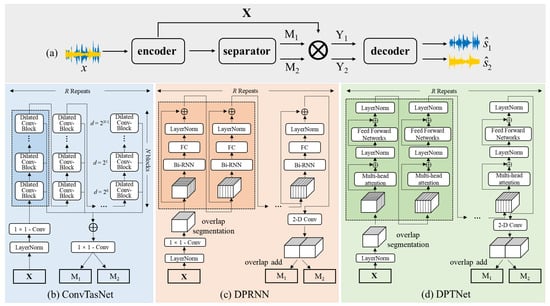
Figure 1.
The structures of three networks, where (a) indicates the unified framework for source separation networks: encoder-separator-decoder, (b–d) indicate the separator in ConvTasNet [15], DPRNN [22], and DPTNet [23], respectively.
The encoder in source separation systems is used to transform the time domain waveform into a non-negative 2-D intermediate representation (X), which is implemented by a 1-D convolutional layer and a rectified linear unit (ReLU) layer. The kernel size (also called window size) in the convolutional layer controls the frame rate of the mixture. It is an essential parameter that affects network performance and is also explored in the section on separation mechanisms. Then separator, the main body of the network, estimates masks for two sources (M1 and M2). The estimated masks are multiplied with X to obtain 2-D representations of each source (Y1 and Y2). Finally, the time-domain signal is reconstructed through the decoder, implemented by a 1-D transposed convolutional layer.
The separator can be implemented through a variety of network structures. The separator in ConvTasNet is a fully convolutional network. At first, input is processed by a global layer normalization (LayerNorm) and a 1 × 1 convolutional layer, indicating a 1-D convolution with a kernel size of 1. It determines the channels for the following modules and is regarded as the bottleneck layer. The main body of ConvTasNet contains R repeated modules (dashed box), and each module is composed of N stacked Dilated Conv-Blocks with exponentially increased dilation factors. Each Dilated Conv-Block is a cascade of 1 × 1 convolution, PReLU, normalization, depth-wise dilated convolution, PReLU, normalization layer. Two 1 × 1 convolutional layers serve as the residual path and the skip-connection path, where the output of the residual path is the input of the next block, and the skip-connection paths of all blocks are summed up and used as the input to a 1 × 1 convolutional layer and a nonlinear activation layer to estimate two masks (M1 and M2).
For the separator in DPRNN, one segmentation stage firstly splits the input X into chunks with overlap and concatenates them to form a 3-D tensor. Then the 3-D tensor is fed to R repeated dual-path recurrent neural modules (dashed box). Each module consists of two submodules that process recurrent connections in different dimensions: intra-chunk and inter-chunk submodules. Each submodule is composed of a Bi-RNN, fully connected layer, and normalization layer. The intra-chunk submodule processes information in each chunk, while the inter-chunk submodule processes global information across chunks. Finally, two estimated 3-D tensors are transformed to 2-D masks through overlap-add methods.
The separator in DPTNet applies the improved Transformer [25] into the dual-path structure. Each improved Transformer (dashed box) includes an intra-Transformer and an inter-Transformer, and each Transformer is composed of a multi-head attention module and a feed-forward network. The multi-head attention module contains multiple scaled dot-product attention modules, an effective self-attention structure. The feed-forward network consists of an RNN followed by a ReLU layer and a fully connected layer.
In this study, these three networks are trained on the same dataset, and whether networks with huge structural differences will learn the same separation mechanisms is explored in Section 4.
3.2. Dataset
In separating two sound sources from a single channel, the network input is the addition of two single sources with different signal-to-noise ratios (SNRs). Because we want to create a similar separation challenge experienced by humans, various types of sounds are considered to build a universal dataset, including speech from LibriSpeech [26], music without vocals from MUSAN [27], and environmental sounds (e.g., animal calls, cars, aircraft, etc.) from the BBC sound effects dataset [28]. All clips were downsampled to 16 kHz and cut to 3 s length. Speech, music, and environmental sounds have the same proportion in our single-source dataset, each with 15,000 clips.
Two source clips were selected randomly and mixed with random signal-to-noise ratios (SNRs) between −5 dB and +5 dB to create mixtures. Mixing clips from the same speaker, the same music tracker, and the same environmental source (e.g., the same car) was not allowed in order to prevent confusion. Overall, there were six different types of mixtures (speech + speech, speech + music, speech + environmental sounds, music + music, music + environmental sounds, and environmental sounds + environmental sounds). The mixture dataset was limited to 180,000 clips (150 h), 70% for training, 20% for cross-validation, and 10% for testing.
3.3. Experiment Configurations
The commonly used scale-invariant source-to-distortion ratio (SI-SDR) [29] is regarded as the training target and evaluation metric. SI-SDR is the difference between the given true source and the estimated source in the time domain,
where , and < > indicates the inner product.
All experiments are based on the Asteroid toolbox [30]. Adam is used as the optimizer with an initial learning rate of 0.001 for 100 epochs. The learning rate is halved if the performance in the validation dataset is not improved in three consecutive epochs. Gradient clipping with a maximum L2-norm of five is applied during training. Except for the window size of filters varied as one important parameter that affects network performance, other hyperparameters of three networks are the same as optimal models reported by three networks [15,22,23] and are shown in Table 1.

Table 1.
Hyperparameters of three networks in our experiments, where “N/A” indicates this parameter is not used in this network.
3.4. Results
The average SI-SDR improvements (SI-SDRi, dB) of the three networks on the test dataset are shown in Table 2. In general, all networks achieved promising results, with DPTNet performing slightly better. Taking one mixture with SI-SDRi of about the average value as an example, spectrograms of the mixture, two clear sources (a female speaker and birds), and two estimated sources obtained by ConvTasNet with 32 sample window size are shown in Figure 2. The SI-SDR improvements of the two estimated sources are 9.39 dB and 12.92 dB, respectively. It can be seen that except for some fine components, most components are well separated and reconstructed. From the perspective of human hearing, these two sources are also well separated and with great intelligibility.
Table 2.
Average SI-SDR improvement (dB) on the test dataset for different networks with different window sizes.
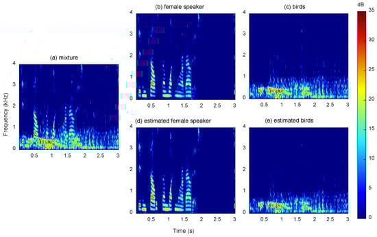
Figure 2.
The spectrogram of (a) mixture, (b,c) two clear sources, (d,e) two estimated sources obtained by ConvTasNet with 32 samples, where two sources are from a female speaker and birds.
In addition to the average SI-SDRi in the entire dataset, the performances of three networks for mixtures with six different types are shown by spider charts with numerical labels in Figure 3. For the separation of speech and other sounds (speech and speech, speech and music, and speech and environmental sounds), the results of the three networks are all significantly better. It means that no matter what kind of network structure is adopted, they can separate sounds with clear structures such as speech. The limited separation between and within environmental sounds and music may be attributed to the following reasons: the music sound here refers to the music pieces rather than individual tones played by one instrument, consisting of a series of instrument tracks. If two music pieces with the same genre are mixed, it is difficult even for humans to separate them. Another reason is that the amount of conveyed information in environmental sounds may not be the same as that of speech, resulting in more difficulties in the separation.
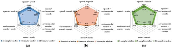
Figure 3.
SI-SDR improvement (dB) of different types for mixtures in the test dataset for (a) ConvTasNet, (b) DPRNN, (c) DPTNet.
As an important parameter that affects network performance, results with different window sizes are also explored. For ConvTasNet, the window size is set to 32, 64, and 128 samples, corresponding to 2, 4, and 8 ms for 16 kHz sample rate, respectively. Due to the introduction of the dual-path processing, the window size is further decreased to two samples in DPRNN and DPTNet, which is extremely hard for traditional fully convolutional layers. Results show that regardless of network structures, separation performances increase as window size decreases. For ConvTasNet and DPTNet, the effect of window size is noticeable, especially for the separation of speech and other sources. For DPRNN, the effect is relatively small and reflected in environmental sounds and music separation. The effect of window size is explained from the perspective of the frequency resolution in Section 4.
4. Separation Mechanisms of Networks
These three trained networks already have the ability to separate universal natural sound sources and with comparable performance in the above natural source dataset. In addition to separation performance, the underlying mechanisms of networks are the primary concern in our study. Do networks learn general principles as human beings? What are the differences in the separation mechanisms learned by different networks? Do the network parameters that affect the separation performance have an impact on the learned principles?
This section answers these questions by exploring the most intuitive primitive principle: proximity. Auditory scene analysis is usually divided into simultaneous and sequential organization [9]. Simultaneous organization groups concurrent components across frequencies, while sequential organization links successive components across time. In this section, the effects of proximity principles in the simultaneous and sequential organization are explored through two classic psychoacoustic experiments and compared with the human auditory system.
4.1. Methods and Stimuli
According to cues to be explored, a series of artificial stimuli are designed as the network input. The network performances (SI-SDRi) are regarded as indicators to analyze the underlying separation mechanisms. There are two main reasons for choosing these simple artificial tones for testing rather than natural sound sources. On the one hand, these stimuli are more controllable, providing the possibility to explore individual cues learned by networks. On the other hand, networks have never been trained by these stimuli. Their separation only relies on general principles learned from unrelated natural sources rather than pattern matching specifically trained sources. All experiments are conducted on these networks trained in Section 3 and without any other fine-tuning and operations.
As shown in Figure 4, two kinds of stimuli are used in simultaneous and sequential organization experiments, respectively. The stimuli for simultaneous organization are two pure tones with different frequency intervals (ΔFs), where tone A varies from 0.1 kHz to 2 kHz in steps of 10 Hz, and ΔF varies from 0 to 2 kHz in steps of 10 Hz. The duration is set to 3 s, including 200 ms raised cosine onset and offset ramps to reduce transient effects. Each frequency component has equal amplitude.
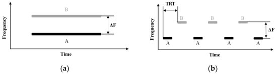
Figure 4.
The schematic spectrogram of the stimuli used in two experiments: (a) simultaneous organization experiments, where A and B indicate two concurrent tones with different frequency intervals (ΔFs). (b) sequential organization experiments, where alternating tones A and B indicate two tones with different frequency intervals (ΔFs) and tone repetition times (TRTs).
The stimuli used in sequential organization experiments are two alternating tones, A and B, with different frequency intervals (ΔFs) and tone repetition times (TRTs, the onset to onset of two adjacent pure tones), as shown in Figure 4b. In order to compare with the temporal coherence boundary, the parameters in van Noorden’s psychoacoustic experiments were replicated. The duration of pure tones A and B is 40 ms, including 5 ms raised cosine onset and offset ramp to reduce transient effects. Pure tone B is fixed at 1 kHz, and ΔF varies from 0 to 15 semitones. The semitone scale is one of the most commonly used scales in psychoacoustic experiments. A semitone is one-twelfth of an octave, and an octave is an interval between one tone and another with double frequency. If is one semitone higher than , . TRT varies from 50 to 200 ms. Each sequence contains a total of 10 A-B tones, and each tone has equal amplitude.
4.2. Proximity in Simultaneous Grouping
For the human auditory system, the perception of two simultaneous tones is one classic simultaneous masking phenomenon, in which the just noticeable level of one sound (maskee) is raised by the presence of another sound (masker) [31]. It can be quantified by the masking amount (dB), which is the raised amount of the just noticeable level [32]. In this study, the masking amount of two pure tones is calculated by MPEG psychoacoustic model 1 [33]. The maximum value of masking amount occurs when the frequencies of two tones are in immediate proximity, and then the masking amount decreases as ΔF increases. When the masking amount is reduced to 0 dB, there is no masking between masker and maskee. The corresponding ΔF is regarded as the separable threshold and drawn by a white dashed curve in Figure 5. For the human auditory system, if ΔF between two components lies under this curve, it will be affected by the masking effect and cannot be perceived as two sources. In contrast, the area above this curve is regarded as the separable range. This separable threshold indicates that the spectral analysis in the human auditory system follows the proximity principle and is good at low frequencies than higher frequencies.
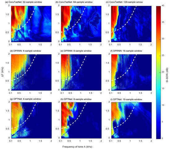
Figure 5.
SI-SDRi (dB) as a function of the frequency of tone A (kHz) and ΔF (kHz), where (a–i) represent results of three well-trained networks (ConvTasNet, DPRNN, and DPTNet) with three different parameters, respectively. The dashed white curve is the ΔF separable threshold at each frequency in the human auditory system.
Results of simultaneous organization experiments for three different networks with three different window sizes are shown in Figure 5. SI-SDRi (dB) is the function of the frequency of tone A and ΔF, where warmer color indicates a better separation. In general, all networks exhibit similar behavioral characteristics as human beings. When ΔF between two tones is large, and tone A is at a lower frequency range (top left corner of each subgraph), components are more likely to be separated. The network separation relies on the frequency proximity of components. More importantly, the separable frequency range (the warmer area) decreases rapidly with frequency increases. The network separation ability at low frequencies is better than at high frequencies. It is highly consistent with the human auditory system, especially for ConvTasNet with a 32-sample window, DPRNN with a 4-sample window, and DPTNet with a 4-sample window. They learn the proximity principle with a similar effective range as humans. For the effective ranges, there are two slight differences worth our attention. One is that networks perform better than humans at low frequencies of 0.1 kHz to 0.2 kHz. The other one is at about 1 kHz, where components still can be separated by humans but cannot be separated by networks.
Although similar auditory behavior characteristics are exhibited, the cues learned by networks with different parameters are slightly different. It has been established in Section 3 that the selection of parameters can affect network performance. The way and extent of parameters’ impact on networks are explored in this experiment. The performance of separating these two simultaneous components with only different frequencies indicates the network frequency resolution. Results show that regardless of network structures, as the window length increases, the frequency selectivity ability of the network decreases. It indicates that the networks with smaller temporal windows have better time resolution and higher frequency resolution. It is the opposite of traditional time-frequency analysis (such as STFT), in which a high spectral resolution requires a long temporal window, resulting in lower temporal resolution. The excellent time-frequency resolution characteristics in these networks can be attributed to the encoder-separator-decoder framework, which convolves with mixtures in the time-domain to obtain the 2-D intermediate representations instead of STFT. For the separator, the introduction of dilated convolution with increasing dilation factors in ConvTasNet ensures a large enough receptive field. Furthermore, the dual-path structure in DPRNN and DPTNet brings a dynamic receptive field, which retains more time-domain information while having higher frequency resolution.
Another phenomenon worth attention is an inseparable blue line with a slope of 1 in the bottom left corner in almost every subgraph. It indicates that when ΔF is equal to the frequency of tone A, the separation of two pure concurrent tones is more difficult. This phenomenon is consistent with the harmonic constraints in the human auditory system, which is also a critical principle for auditory scene analysis [34]. When components have a harmonic relationship (the frequency of one component is twice that of another component), they will be regarded as coming from the same sound source and inseparable in perception.
Furthermore, the harmonicity effect line occurs at low frequencies for all networks. For the human auditory system, higher-order harmonics also cannot be resolved and results in less harmonic constraints at high frequencies. In addition, the harmonic effect line lies in the inseparable range, which is under the white dashed curve. It indicates that although the surrounding points cannot be separated due to the proximity principle, these cases that are in harmonic will be more challenging to separate. It reflects the interaction of proximity and harmonicity principles. The significance of the harmonic effect line in each subgraph reflects the network’s weights impacted on proximity and harmonicity principles. For ConvTasNet, the harmonic effect line is not significant enough. It may be because the network is more sensitive to the proximity principle, while for DPRNN and DPTNet, the harmonic effect lines can be seen effortlessly. For DPRNN with a 4-sample window, there is even another inseparable line with a 3:1 frequency ratio.
In summary, there are three contributions from this experiment. First, regardless of network structures and parameters, the proximity principle in frequency is learned spontaneously by these networks. There is no correlation between these networks because their structure and parameters are different. After training on the same dataset in Section 3, all networks showed similar performance in this proximity experiment, which is also consistent with the performance of the human auditory system (the white dashed curve). It implies that the learned principles are not accidental but the optimal strategies selected by networks when facing the same separation task. Second, the comparison of networks with different parameters helps us understand the resolution ability of networks. It illustrates that a network with a small window size has a better frequency resolution and explains why networks with smaller window sizes perform better for universal source separation in Section 3. It provides experimental support for parameter selection and subsequent network optimization and benefits the explanation of the “black box” of networks. Third, in addition to the proximity principle, other factors such as harmonicity also contribute to the segregation or integration of components. The interaction between different cues is also worthy of our attention.
4.3. Proximity in Sequential Grouping
Results of sequential organization experiments for alternating tones A and B are shown in Figure 6. In general, no matter which structure and parameter are used, the proximity in time and frequency for sequential grouping is learned by all networks. When ΔF is large, and TRT is short (top left corner of each subgraph), sequences A and B are more likely to be separated. The temporal coherence boundary proposed by van Noorden [21] through psychoacoustical experiments is shown by the white dashed curve in Figure 6. For the human auditory system, when the tone interval is higher than the temporal coherence boundary, they will be perceived as two sources. Therefore, for proximity in the sequential grouping, the networks also show a high degree of consistency with humans.
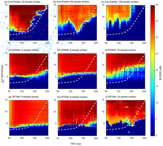
Figure 6.
SI-SDRi (dB) as a function of TRT (ms) and ΔF (semitones), where (a–i) represent results of three well-trained networks (ConvTasNet, DPRNN, and DPTNet) with three different parameters, respectively. The dashed white curve indicates the temporal coherence boundary in the human auditory system.
Although the proximity principle is embodied in each subgraph, there are some differences in different structures and parameters. ConvTasNet with a 32-sample window fits best with the temporal coherence boundary. As the window size increases, the separation range on TRT and ΔF decreases. DPRNN and DPTNet are more sensitive to frequency intervals rather than time intervals. DPTNet with a 4-sample window will separate components larger than a certain frequency interval (about five semitones) regardless of the time interval. In general, the performances of DPRNN and DPTNet are better than ConvTasNet for this sequential grouping experiment.
In our previous attempt [18] to unravel underlying separation principles learned by networks, results showed that the proximity principle could be learned by ConvTasNet with different encoders. Furthermore, in this study, the proximity principle is still effective for different network structures and parameters. It indicates that in the face of such tasks, the separation based on proximity principles may be one optimal and inevitable choice. No matter what kind of network, even the human ear, the same separation mechanisms will eventually be chosen to solve this problem.
5. Discussion
Recently, many networks have been proposed and have made significant progress, even reaching human-level performance [10]. However, the study of the underlying mechanisms is still in its infancy [35]. In this study, different from the visualization of filter or feature map in intermediate layers, the mechanisms of network behavior in the higher level are explained. The effects of network structure and parameters on frequency resolution are quantitatively analyzed through the proximity experiment, providing a new method to explain the “black box” of deep networks from the perspective of auditory perception mechanisms.
To our knowledge, it is the first demonstration that regardless of network structures and parameters, the same auditory separation mechanisms are learned by networks from unrelated nature sources. These networks based on CNN, RNN, or Transformer are purely statistical models and do not specifically model the auditory periphery and cortical processing or extract specific auditory attributes. Although only the proximity principle is explored in this study due to the limited space, the emergence of the harmonic effect line in the simultaneous experiment suggests that networks are likely to learn other auditory-like principles. In addition, the difference in network frequency-selective ability at low and high frequencies also illustrates the biological plausibility of the networks. It motivates us to think further about the deep networks and auditory system.
Is the destination of deep separation networks to learn the same mechanisms as human beings? All three networks with different structures in our study have achieved this in some respects spontaneously. This result implies that the behavior characteristics of human auditory scene analysis can be understood as consequences of optimization for the selective listening task in natural environments. Humans may have chosen the optimal strategy under environmental constraints. When facing the same challenges, networks also tend to learn this optimal strategy from statistical regularities. Francl and McDermott [36] illustrated that a deep network replicated some key characteristics of human sound localization. Kell et al. [35] demonstrated that a deep network optimized to recognize speech and music replicated some human auditory behavior and predicted brain responses. In our study, in the separation task, networks also mimic the human auditory system spontaneously.
6. Conclusions and Future Work
In this study, an ill-posed perceptual problem, two sources separation in monaural recordings, is addressed. Three different networks with different parameters are trained by a universal dataset and achieve excellent performances. More importantly, the most intuitive principle, proximity, is explored in simultaneous and sequential grouping experiments, respectively. Results show that the behavior characteristics of all networks are highly consistent with that of the human auditory system. If components are proximate in frequency or time, they are not easily separated by networks. Furthermore, the frequency resolution at low frequencies is better than at high frequencies.
This study has a profound impact on deep learning and the auditory system. Instead of imitating specific structures such as the auditory periphery or cortex, the higher-level behavior characteristics of humans are simulated through optimization processes. Because networks are based on general principles similar to those in humans, it is possible to develop a universal system that can be adapted to all sources and various scenes or even adapted to multiple tasks simultaneously, such as the joint task of separation and recognition. It provides the possibility to achieve the remarkable ability of the human ear in many aspects such as separation, recognition, and location through deep learning and lays a scientific foundation for solving the holy grail of machine listening.
Our study is the first step that explores the underlying mechanisms from the auditory system, while the network structures and parameters cannot be exhausted. More principles (such as common fate) and the interaction of principles also deserve further exploration. In addition, it is still an open question whether the characteristics of the training dataset determine the principles learned by networks. If certain components, such as those at high frequencies in datasets, are deliberately strengthened, the network may also be sensitive to the high-frequencies. It is similar to the schema-based principles in the human auditory system, which rely on knowledge or attention. It provides the possibility that a more flexible network in specific scenes can be obtained.
Author Contributions
Conceptualization, H.L. and L.W.; methodology, H.L.; software, H.L.; validation, J.L., B.W., and B.Z.; formal analysis, L.W.; investigation, H.L.; resources, J.L.; data curation, B.Z.; writing—original draft preparation, H.L.; writing—review and editing, K.C.; visualization, H.L.; supervision, K.C.; project administration, K.C.; funding acquisition, K.C. All authors have read and agreed to the published version of the manuscript.
Funding
This research was funded by the Open Fund of State Key Laboratory of Power Grid Environmental Protection, grant number GYW51201001554.
Conflicts of Interest
The authors declare no conflict of interest.
References
- Narayanan, A.; Wang, D.L. Investigation of speech separation as a front-end for noise robust speech recognition. IEEE Trans. Audio Speech Lang. Process. 2014, 22, 826–835. [Google Scholar] [CrossRef]
- Ephrat, A.; Mosseri, I.; Lang, O.; Dekel, T.; Wilson, K.; Hassidim, A.; Freeman, W.T.; Rubinstein, M. Looking to listen at the cocktail party: A speaker-independent audio-visual model for speech separation. ACM Trans. Graph. 2018, 37, 1–11. [Google Scholar] [CrossRef]
- Borgström, B.J.; Brandstein, M.S.; Ciccarelli, G.A.; Quatieri, T.F.; Smalt, C.J. Speaker separation in realistic noise environments with applications to a cognitively-controlled hearing aid. Neural Netw. 2021, 140, 136–147. [Google Scholar] [CrossRef] [PubMed]
- Adavanne, S.; Politis, A.; Nikunen, J.; Virtanen, T. Sound event localization and detection of overlapping sources using convolutional recurrent neural networks. IEEE J. Sel. Top. Signal Process. 2019, 13, 34–48. [Google Scholar] [CrossRef]
- Anwar, M.Z.; Kaleem, Z.; Jamalipour, A. Machine learning inspired sound-based amateur drone detection for public safety applications. IEEE Trans. Veh. Technol. 2019, 68, 2526–2534. [Google Scholar] [CrossRef]
- Marchegiani, L.; Posner, I. Leveraging the urban soundscape: Auditory perception for smart vehicles. In Proceedings of the IEEE International Conference on Robotics and Automation, Singapore, 29 May–3 June 2017; pp. 6547–6554. [Google Scholar]
- Li, H.; Chen, K.; Seeber, B.U. ConvTasNet-based anomalous noise separation for intelligent noise monitoring. In Proceedings of the 2021 International Congress and Exposition of Noise Control Engineering, Washington, DC, USA, 1–5 August 2021; pp. 2044–2051. [Google Scholar]
- Sawata, R.; Uhlich, S.; Takahashi, S.; Mitsufuji, Y. All for one and one for all: Improving music separation by bridging Networks. In Proceedings of the IEEE International Conference on Acoustics, Speech and Signal Processing (ICASSP), Toronto, ON, Canada, 6–11 June 2021; pp. 51–55. [Google Scholar]
- Wang, D.; Brown, G.J. Computational Auditory Scene Analysis: Principles, Algorithms, and Applications; Wiley-IEEE Press: Hoboken, NJ, USA, 2006; ISBN 9781848210318. [Google Scholar]
- Wang, D.; Chen, J. Supervised speech separation based on deep learning: An overview. IEEE/ACM Trans. Audio Speech Lang. Process. 2018, 26, 1702–1726. [Google Scholar] [CrossRef] [PubMed]
- Grossberg, S.; Govindarajan, K.K.; Wyse, L.L.; Cohen, M.A. ARTSTREAM: A neural network model of auditory scene analysis and source segregation. Neural Netw. 2004, 17, 511–536. [Google Scholar] [CrossRef] [PubMed]
- Hu, G.; Wang, D. Auditory segmentation based on onset and offset analysis. IEEE Trans. Audio Speech Lang. Process. 2007, 15, 396–405. [Google Scholar] [CrossRef]
- Hu, G.; Wang, D. Monaural speech segregation based on pitch tracking and amplitude modulation. IEEE Trans. Neural Netw. 2004, 15, 1135–1150. [Google Scholar] [CrossRef] [PubMed]
- Kavalerov, I.; Wisdom, S.; Erdogan, H.; Patton, B.; Wilson, K.; Le Roux, J.; Hershey, J.R. Universal sound separation. In Proceedings of the IEEE Workshop on Applications of Signal Processing to Audio and Acoustics, New Paltz, NY, USA, 20–23 October 2019; pp. 175–179. [Google Scholar]
- Luo, Y.; Mesgarani, N. Conv-TasNet: Surpassing ideal Time-Frequency magnitude masking for speech separation. IEEE/ACM Trans. Audio Speech Lang. Process. 2019, 27, 1256–1266. [Google Scholar] [CrossRef] [PubMed]
- Kang, S.; Park, J.-S.; Jang, G.-J. Improving singing voice separation using curriculum learning on recurrent neural networks. Appl. Sci. 2020, 10, 2465. [Google Scholar] [CrossRef]
- Li, H.; Chen, K.; Li, R.; Liu, J.; Wan, B.; Zhou, B. Auditory-like simultaneous separation mechanisms spontaneously learned by a deep source separation network. Appl. Acoust. 2022, 188, 108591. [Google Scholar] [CrossRef]
- Li, H.; Chen, K.; Seeber, B.U. Auditory filterbanks benefit universal sound source separation. In Proceedings of the IEEE International Conference on Acoustics, Speech and Signal Processing (ICASSP), Toronto, ON, Canada, 6–11 June 2021; pp. 181–185. [Google Scholar]
- Bregman, A.S. Auditory Scene Analysis: The Perceptual Organization of Sound; MIT Press: Cambridge, UK, 1990; ISBN 0-262-02297-4. [Google Scholar]
- Fastl, H.; Zwicker, E. Psychoacoustics: Facts and Models, 3rd ed.; Springer Science & Business Media: New York, NY, USA, 2007; ISBN 9783642084638. [Google Scholar]
- van Noorden, L.S. Temporal Coherence in the Perception of Tone Sequences; Technische Hogeschool Eindhoven: Eindhoven, The Netherlands, 1975. [Google Scholar]
- Luo, Y.; Chen, Z.; Yoshioka, T. Dual-Path RNN: Efficient long sequence modeling for time-domain single-channel speech separation. In Proceedings of the IEEE International Conference on Acoustics, Speech and Signal Processing (ICASSP), Barcelona, Spain, 4–8 May 2020; pp. 46–50. [Google Scholar]
- Chen, J.; Mao, Q.; Liu, D. Dual-Path Transformer network: Direct context-aware modeling for end-to-end monaural speech separation. In Proceedings of the INTERSPEECH, Shanghai, China, 25–29 October 2020; pp. 2642–2646. [Google Scholar]
- Shrestha, A.; Mahmood, A. Review of deep learning algorithms and architectures. IEEE Access 2019, 7, 53040–53065. [Google Scholar] [CrossRef]
- Vaswani, A.; Brain, G.; Shazeer, N.; Parmar, N.; Uszkoreit, J.; Jones, L.; Gomez, A.N.; Kaiser, Ł.; Polosukhin, I. Attention Is All You Need. In Proceedings of the Neural Information Processing Systems, Long Beach, CA, USA, 4–7 December 2017; pp. 5998–6008. [Google Scholar]
- Panayotov, V.; Chen, G.; Povey, D.; Khudanpur, S. Librispeech: An ASR corpus based on public domain audio books. In Proceedings of the IEEE International Conference on Acoustics, Speech and Signal Processing (ICASSP), South Brisbane, QLD, Australia, 19–24 April 2015; pp. 5206–5210. [Google Scholar]
- Snyder, D.; Chen, G.; Povey, D. MUSAN: A music, speech, and noise corpus. arXiv 2015, arXiv:1510.08484. [Google Scholar]
- BBC. BBC Sound Effects—Research & Education Space. Available online: http://bbcsfx.acropolis.org.uk/ (accessed on 23 June 2020).
- Roux, J.L.; Wisdom, S.; Erdogan, H.; Hershey, J.R. SDR—Half-baked or well done? In Proceedings of the IEEE International Conference on Acoustics, Speech and Signal Processing (ICASSP), Brighton, UK, 12–17 May 2019; pp. 626–630. [Google Scholar]
- Pariente, M.; Cornell, S.; Cosentino, J.; Sivasankaran, S.; Tzinis, E.; Heitkaemper, J.; Olvera, M.; Stöter, F.-R.; Hu, M.; Martín-Doñas, J.M.; et al. Asteroid: The PyTorch-based audio source separation toolkit for researchers. In Proceedings of the INTERSPEECH, Shanghai, China, 25–29 October 2020; pp. 2637–2641. [Google Scholar]
- ANSI S1.1-1994; American National Standard Acoustical Terminology. American National Standards Institute: New York, NY, USA, 1994.
- Gelfand, S.A. Hearing: An Introduction to Psychological and Physiological Acoustics, 4th ed.; Informa Healthcare: London, UK, 2004; ISBN 9780824757274. [Google Scholar]
- ISO/IEC 11172-3; Information Technology—Coding of Moving Pictures and Associated Audio for Digital Storage Media at Up to 1.5 Mbits/s—Part 3: Audio. ISO/IEC: Geneva, Switzerland, 1993; pp. 1–154.
- Micheyl, C.; Oxenham, A.J. Pitch, harmonicity and concurrent sound segregation: Psychoacoustical and neurophysiological findings. Hear. Res. 2010, 266, 36–51. [Google Scholar] [CrossRef] [PubMed][Green Version]
- Kell, A.J.E.; Yamins, D.L.K.; Shook, E.N.; Norman-Haignere, S.V.; McDermott, J.H. A Task-optimized neural network replicates human auditory behavior, predicts brain responses, and reveals a cortical processing hierarchy. Neuron 2018, 98, 630–644.e16. [Google Scholar] [CrossRef]
- Francl, A.; McDermott, J.H. Deep neural network models of sound localization reveal how perception is adapted to real-world environments. bioRxiv 2020, 1–46. [Google Scholar] [CrossRef]
Publisher’s Note: MDPI stays neutral with regard to jurisdictional claims in published maps and institutional affiliations. |
© 2022 by the authors. Licensee MDPI, Basel, Switzerland. This article is an open access article distributed under the terms and conditions of the Creative Commons Attribution (CC BY) license (https://creativecommons.org/licenses/by/4.0/).