
Retrieval of Chlorophyll-a Concentrations in the Coastal Waters of the Beibu Gulf in Guangxi Using a Gradient-Boosting Decision Tree Model

Abstract
:1. Introduction
2. Materials and Methods
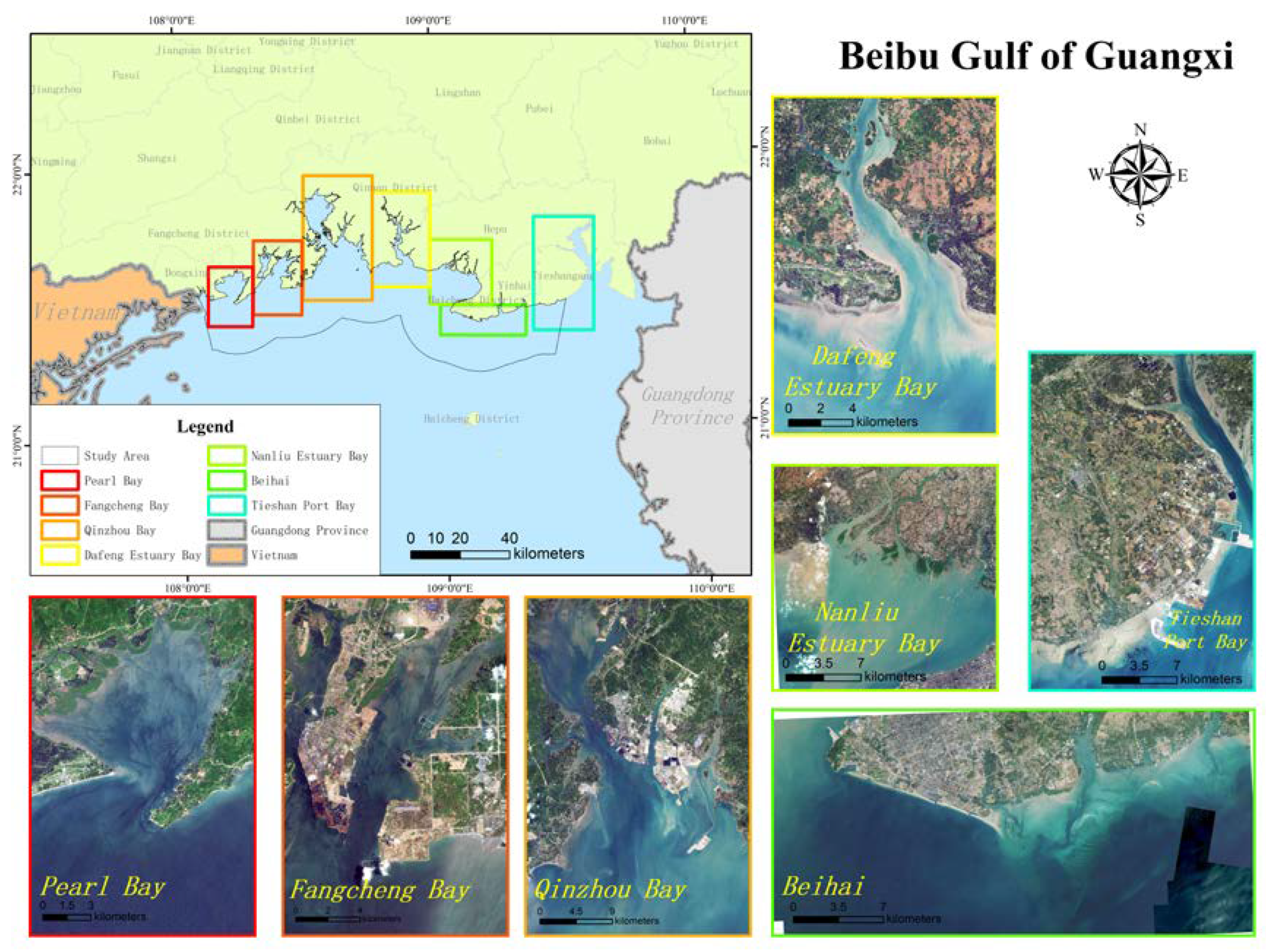
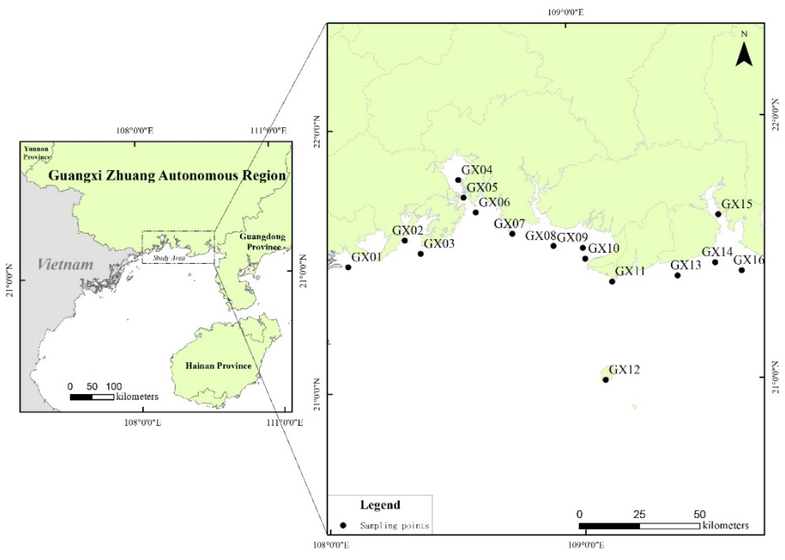
2.1. Study Area
2.2. Dataset
2.2.1. In Situ Data
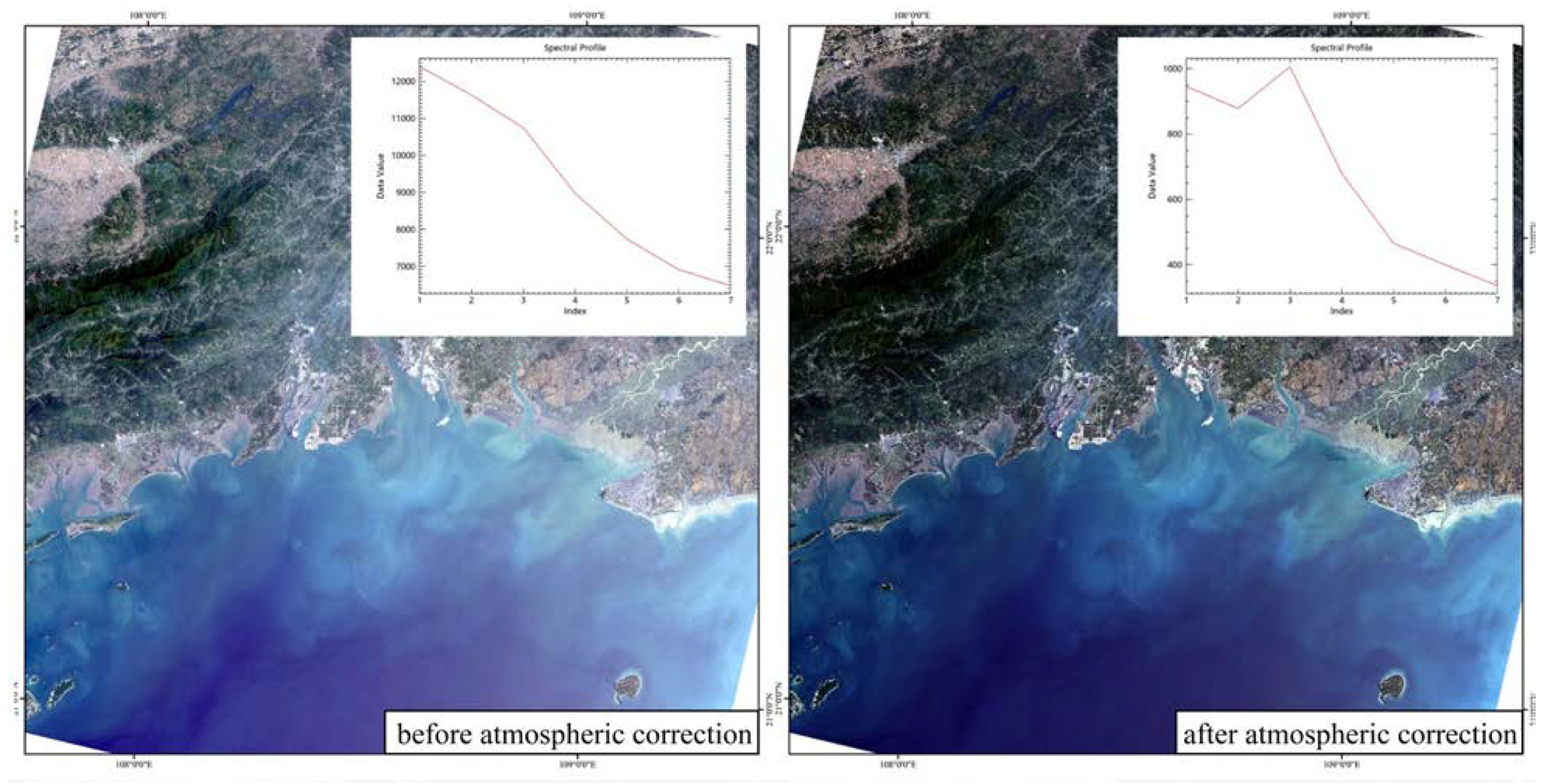
2.2.2. Satellite Data Acquisition and Pre-Processing
2.2.3. Calibration Dataset
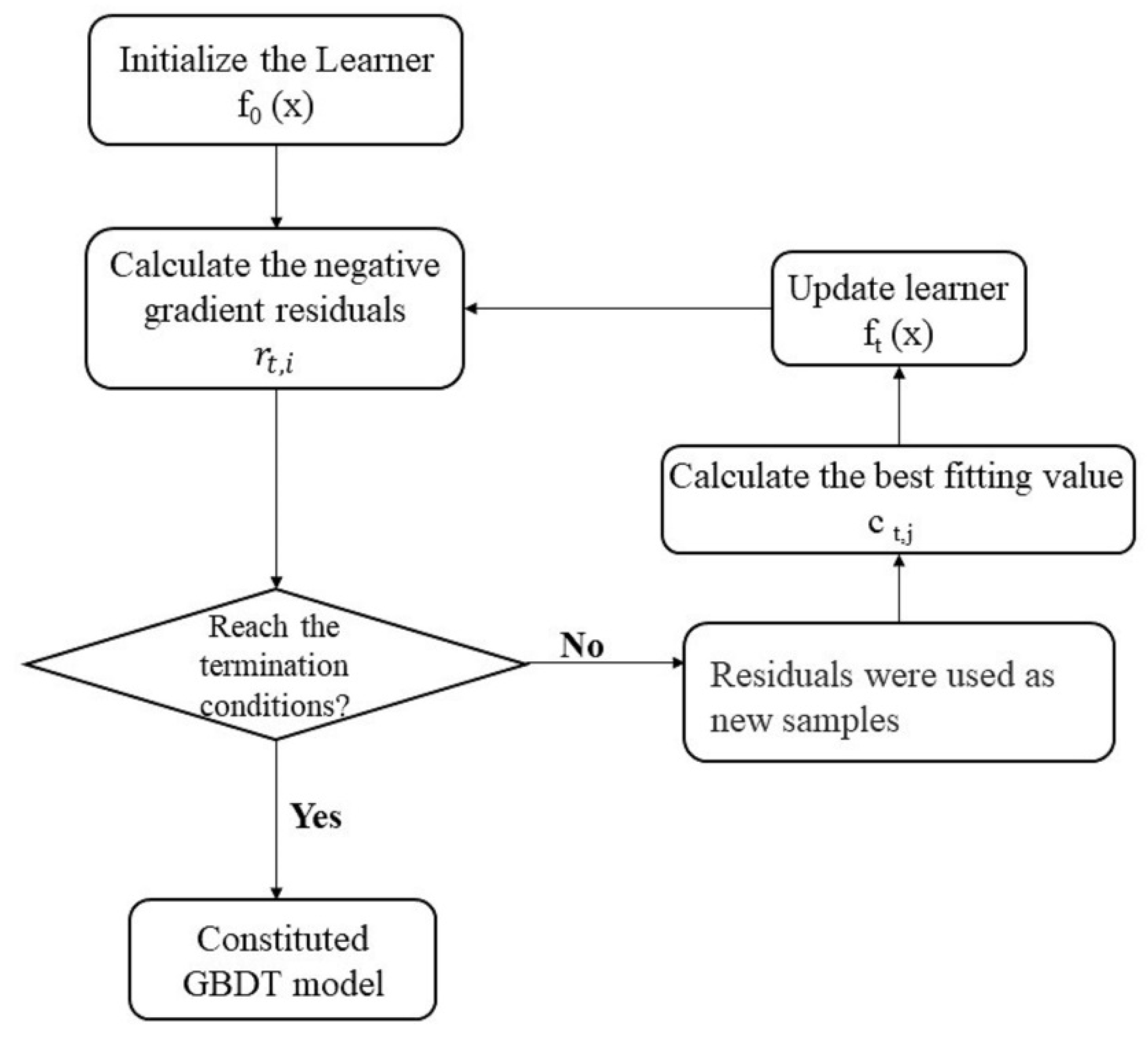
2.3. GBDT Model
3. Results
3.1. Performance Assessment
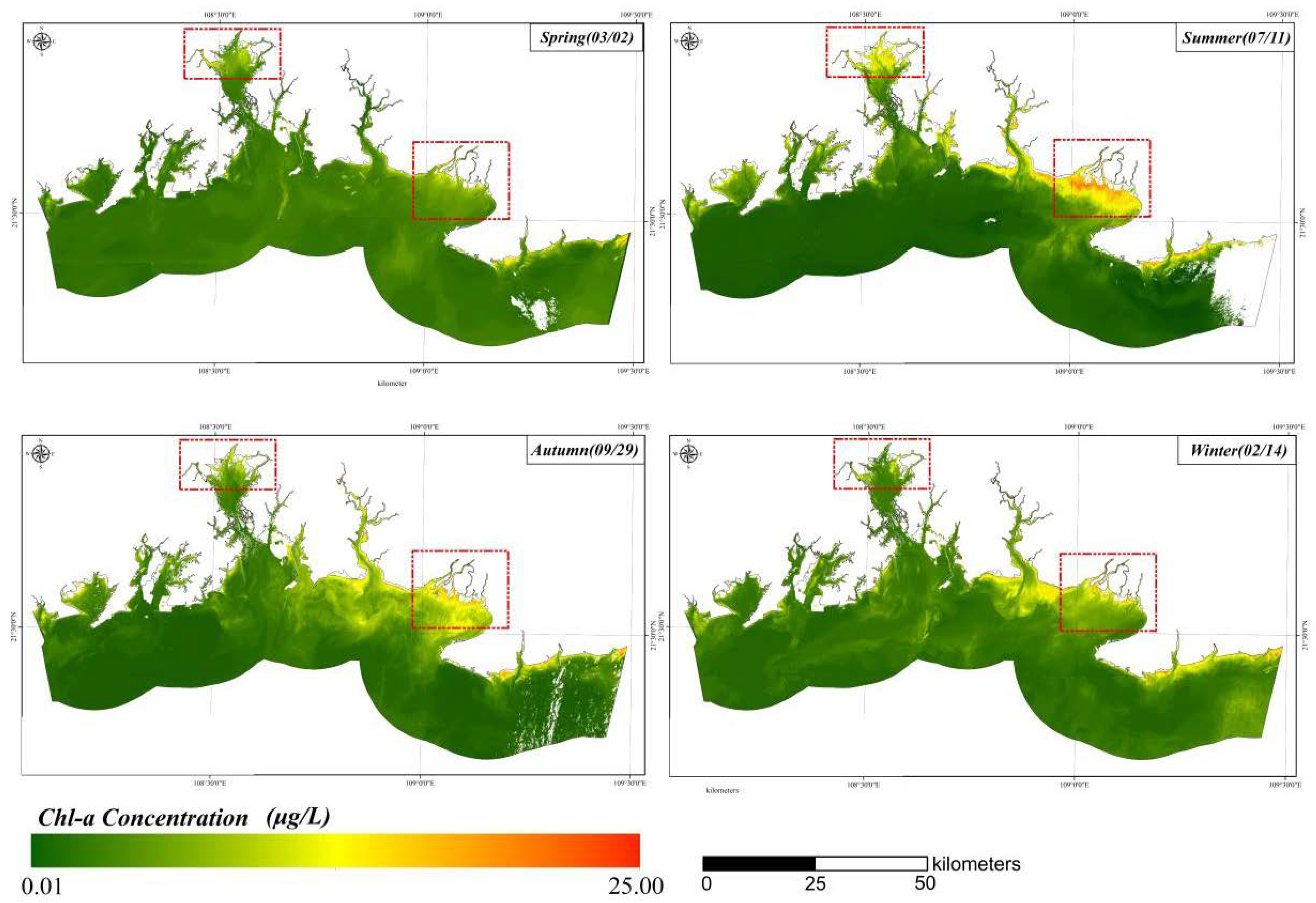
3.2. Spatial–Temporal Distribution of Chl-a
3.2.1. Spatial Variations of Chl-a
3.2.2. Temporal Variations of Chl-a
3.3. Theil–Sen and Mann-Kendall Trend Analysis
4. Discussion
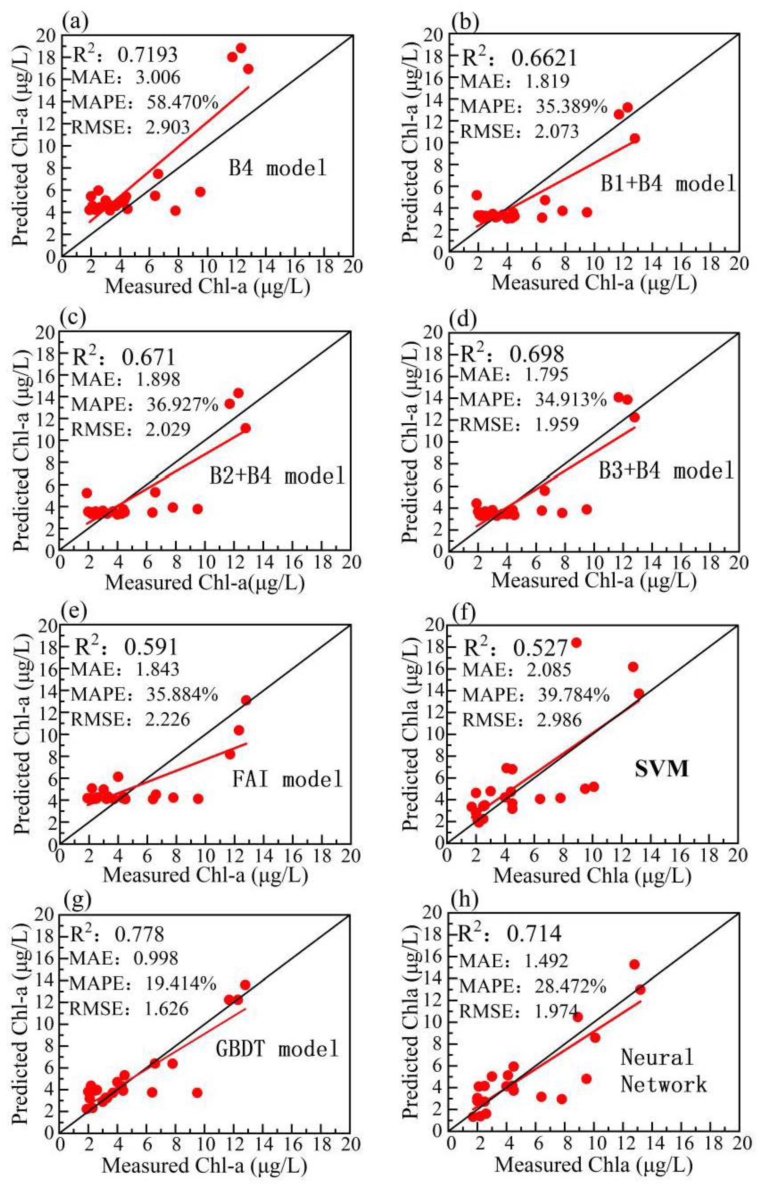
4.1. Comparison of Different Models
4.2. Spatial and Temporal Distribution of Chl-a
4.2.1. Spatial Difference of Chl-a
4.2.2. Temporal Variation of Chl-a
5. Conclusions
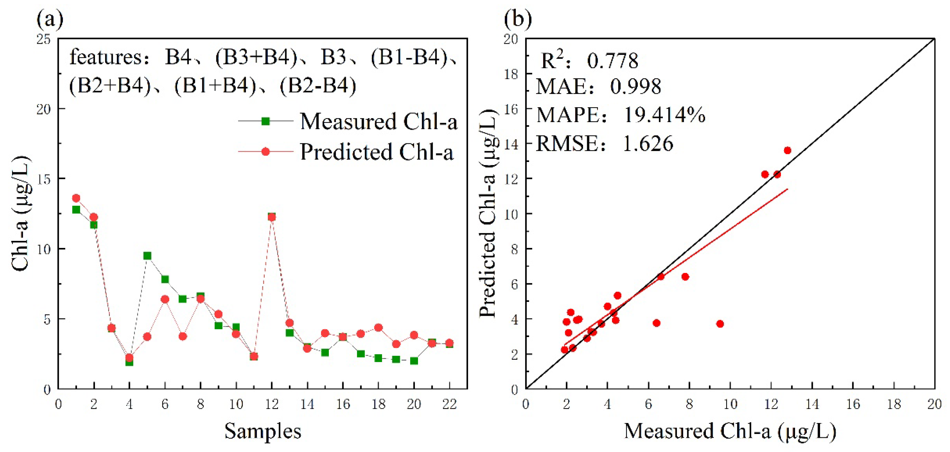
- Compared with the performance of different models, the GBDT model can significantly improve the accuracy of Chl-a concentration inversion, proving that it can be a new method for remote sensing inversion of the water quality parameters. When B4, B3 + B4, B3, B1 − B4, B2 + B4, B1 + B4, and B2 − B4 were considered the characteristic variables of the GBDT model, the inversion accuracy of the model was the highest (MAE = 0.998 μg/L, MAPE = 19.413%, RMSE = 1.626 μg/L, and R2 = 0.778).
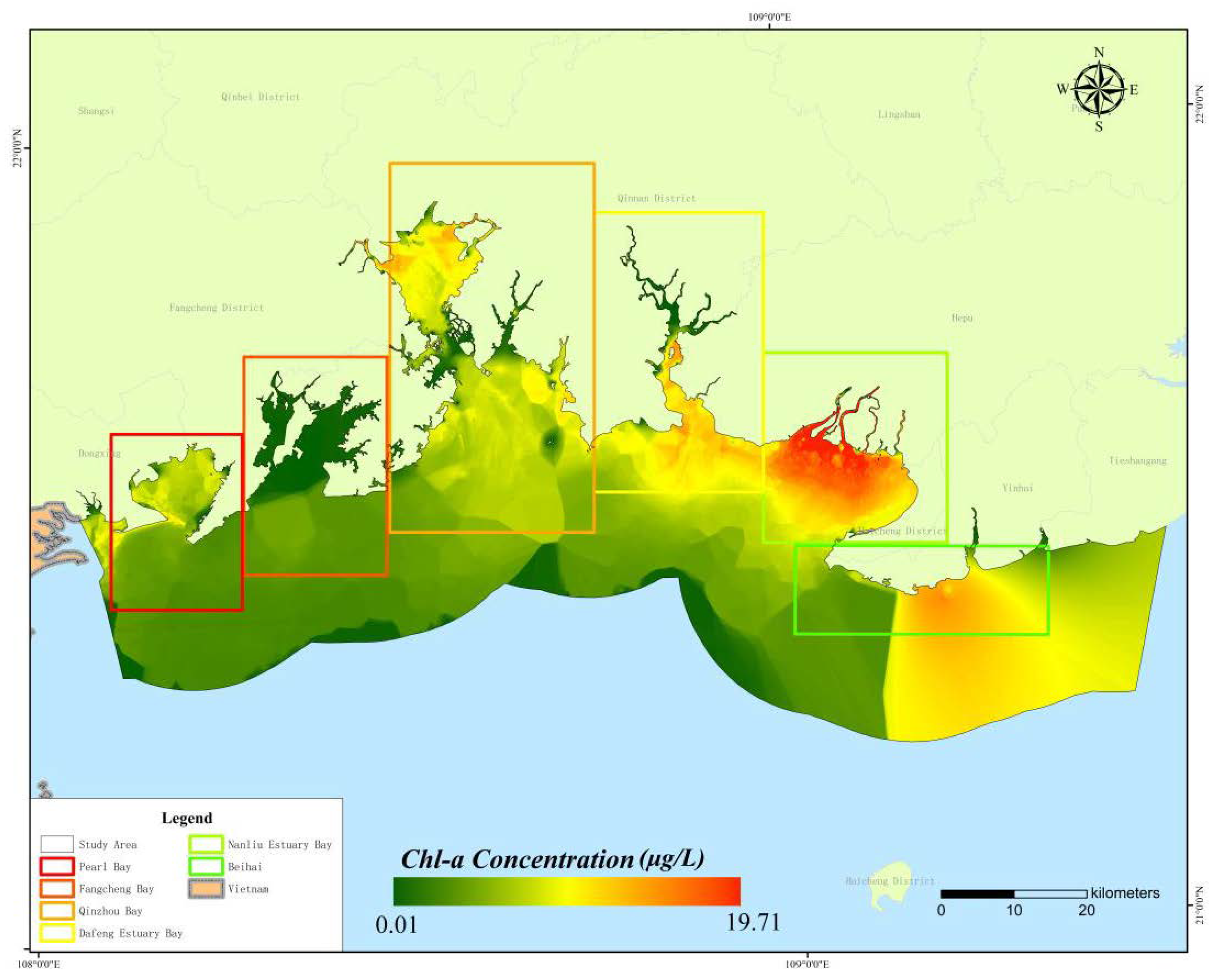
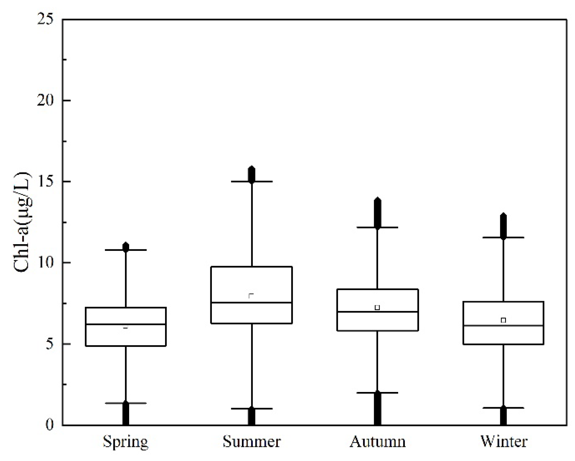
- The spatial distribution of the Chl-a concentration was highest in the nearshore and lowest in the offshore waters in the Beibu Gulf in Guangxi. The Chl-a concentration was highest in the summer, and the concentration in autumn was lower, while concentrations in spring and winter were the lowest. The ranking of Chl-a concentrations, from high to low, across multiple bays was as follows: Nanliu River Estuary Bay, Dafeng River Estuary Bay, Qinzhou Bay, Beihai Pearl Harbor, and Fangcheng Bay.
Author Contributions
Funding
Institutional Review Board Statement
Informed Consent Statement
Data Availability Statement
Conflicts of Interest
References
- Brooks, B.W.; Lazorchak, J.M.; Howard, M.D.A.; Johnson, M.V.; Morton, S.L.; Perkins, D.A.K.; Reavie, E.D.; Scott, G.I.; Smith, S.A.; Steevens, J.A. Are harmful algal blooms becoming the greatest inland water quality threat to public health and aquatic ecosystems? Environ. Toxicol. Chem. 2016, 35, 6–13. [Google Scholar] [CrossRef]
- Carmichael, W.W. Health effects of toxin-producing cyanobacteria: “The CyanoHABs”. Hum. Ecol. Risk Assess. 2001, 7, 1393–1407. [Google Scholar] [CrossRef]
- Carvalho, L.; McDonald, C.; de Hoyos, C.; Mischke, U.; Phillips, G.; Borics, G.; Poikane, S.; Skjelbred, B.; Solheim, A.L.; Van Wichelen, J.; et al. Sustaining recreational quality of European lakes: Minimizing the health risks from algal blooms through phosphorus control. J. Appl. Ecol. 2013, 50, 315–323. [Google Scholar] [CrossRef] [Green Version]
- Duan, H.; Ma, R.; Xu, X.; Kong, F.; Zhang, S.; Kong, W.; Hao, J.; Shang, L. Two-Decade Reconstruction of Algal Blooms in China’s Lake Taihu. Environ. Sci. Technol. 2009, 43, 3522–3528. [Google Scholar] [CrossRef]
- Gao, D.; Li, C.; Liu, G.; Zhang, H. The species composition and distribution of phytoplankton in the Beibu Bay. J. Zhanjiang Ocean Univ. 2001, 21, 13–18. [Google Scholar]
- Dörnhöfer, K.; Klinger, P.; Heege, T.; Oppelt, N. Multi-sensor satellite and in situ monitoring of phytoplankton development in a eutrophic-mesotrophic lake. Sci. Total Environ. 2018, 612, 1200–1214. [Google Scholar] [CrossRef]
- Li, X.; Wei, A.; Jiang, S.; Wang, T.; Ji, X.; Zhang, Y.; Jiao, X. Retrieval of chlorophyll-a and total suspended matter concentrations from sentinel-3OLCI imagery by C2RCC algorithm in south yellow sea. Environ. Monit. 2020, 12, 6–12. [Google Scholar]
- Li, Y.; Huang, J.; Wei, Y.; Lu, W. Inversing Chlorophyll Concentration of Taihu Lake by Analytic Model. Natl. Remote Sens. Bull. 2006, 10, 169–175. [Google Scholar]
- Yang, W.; Chen, J.; Mausushita, B. Algorithm for Estimating Chlorophyll-a Concentration in Case II Water Body Based on Bio-Optical Model. Spectrosc. Spectr. Anal. 2009, 29, 38–42. [Google Scholar]
- Chang, N.; Imen, S.; Vannah, B. Remote Sensing for Monitoring Surface Water Quality Status and Ecosystem State in Relation to the Nutrient Cycle: A 40-Year Perspective. Crit. Rev. Environ. Sci. Technol. 2015, 45, 101–166. [Google Scholar] [CrossRef]
- Sagan, V.; Peterson, K.T.; Maimaitijiang, M.; Sidike, P.; Sloan, J.; Greeling, B.A.; Maalouf, S.; Adams, C. Monitoring inland water quality using remote sensing: Potential and limitations of spectral indices, bio-optical simulations, machine learning, and cloud computing. Earth-Sci. Rev. 2020, 205, 103187. [Google Scholar] [CrossRef]
- Cao, Z.; Ma, R.; Duan, H.; Pahlevan, N.; Melack, J.; Shen, M.; Xue, K. A machine learning approach to estimate chlorophyll-a from Landsat-8 measurements in inland lakes. Remote Sens. Environ. 2020, 248, 111974. [Google Scholar] [CrossRef]
- Xue, K.; Zhang, Y.; Duan, H.; Ma, R.; Loiselle, S.; Zhang, M. A Remote Sensing Approach to Estimate Vertical Profile Classes of Phytoplankton in a Eutrophic Lake. Remote Sens. 2015, 7, 14403–14427. [Google Scholar] [CrossRef] [Green Version]
- Pyo, J.; Duan, H.; Baek, S.; Kim, M.S.; Jeon, T.; Kwon, Y.S.; Lee, H.; Cho, K.H. A convolutional neural network regression for quantifying cyanobacteria using hyperspectral imagery. Remote Sens. Environ. 2019, 233, 111350. [Google Scholar] [CrossRef]
- Liu, H.; Yan, L. Back-Propagation Network Model for Predicting the Change of Eutrophication of Qiandao Lake. Bull. Sci. Technol. 2008, 24, 411–416. [Google Scholar]
- Li, S.; Song, K.; Wang, S.; Liu, G.; Wen, Z.; Shang, Y.; Lyu, L.; Chen, F.; Xu, S.; Tao, H.; et al. Quantification of chlorophyll-a in typical lakes across China using Sentinel-2 MSI imagery with machine learning algorithm. Sci. Total Environ. 2021, 778, 146271. [Google Scholar] [CrossRef] [PubMed]
- Deng, L.; Zhou, W.; Cao, W.; Zheng, W.; Wang, G.; Xu, Z.; Li, C.; Yang, Y.; Hu, S.; Zhao, W. Retrieving Phytoplankton Size Class from the Absorption Coefficient and Chlorophyll A Concentration Based on Support Vector Machine. Remote Sens. 2019, 11, 1054. [Google Scholar] [CrossRef] [Green Version]
- Peterson, K.T.; Sagan, V.; Sidike, P.; Cox, A.L.; Martinez, M. Suspended Sediment Concentration Estimation from Landsat Imagery along the Lower Missouri and Middle Mississippi Rivers Using an Extreme Learning Machine. Remote Sens. 2018, 10, 1503. [Google Scholar] [CrossRef] [Green Version]
- Gonzalez Vilas, L.; Spyrakos, E.; Torres Palenzuela, J.M. Neural network estimation of chlorophyll a from MERIS full res-olution data for the coastal waters of Galician rias (NW Spain). Remote Sens. Environ. 2011, 115, 524–535. [Google Scholar] [CrossRef]
- Pahlevan, N.; Smith, B.; Schalles, J.; Binding, C.; Cao, Z.; Ma, R.; Alikas, K.; Kangro, K.; Gurlin, D.; Nguyen, H.; et al. Seamless retrievals of chlorophyll-a from Sentinel-2 (MSI) and Sentinel-3 (OLCI) in inland and coastal waters: A ma-chine-learning approach. Remote Sens. Environ. 2020, 240, 111604. [Google Scholar] [CrossRef]
- Wang, Q.; Chen, D.; Gao, X.; Wang, F.; Li, J.; Liao, W.; Wang, Z.; Xie, G. Microscopic pore structures of tight sandstone reservoirs and their diagenetic controls: A case study of the Upper Triassic Xujiahe Formation of the Western Sichuan Depression, China. Mar. Petrol. Geol. 2020, 113, 104119. [Google Scholar] [CrossRef]
- Sagi, O.; Rokach, L. Approximating XGBoost with an interpretable decision tree. Inform. Sci. 2021, 572, 522–542. [Google Scholar] [CrossRef]
- Zhang, J.; Liang, Q.; Jiang, R.; Li, X. A Feature Analysis Based Identifying Scheme Using GBDT for DDoS with Multiple Attack Vectors. Appl. Sci. 2019, 9, 4633. [Google Scholar] [CrossRef] [Green Version]
- Wang, C.; Zhang, J.; Yu, G. Cluster Analysis of Pedestrian Mobile Channels in Measurements and Simulations. Appl. Sci. 2019, 9, 886. [Google Scholar] [CrossRef] [Green Version]
- Kawatani, T.; Yamaguchi, T.; Sato, Y.; Maita, R.; Mine, T. Prediction of Bus Travel Time over Intervals between Pairs of Adjacent Bus Stops Using City Bus Probe Data. Int. J. Intell. Transp. Syst. Res. 2021, 19, 456–467. [Google Scholar]
- Hou, C.; Cao, B.; Fan, J. A data-driven method to predict service level for call centers. IET Commun. 2021, 2, 1–12. [Google Scholar] [CrossRef]
- Sun, R.; Wang, G.; Cheng, Q.; Fu, L.; Chiang, K.; Hsu, L.; Ochieng, W.Y. Improving GPS Code Phase Positioning Accuracy in Urban Environments Using Machine Learning. IEEE Internet Things J. 2021, 8, 7065–7708. [Google Scholar] [CrossRef]
- Huang, P.; Wang, L.; Hou, D.; Lin, W.; Yu, J.; Zhang, G.; Zhang, H. A feature extraction method based on the entropy-minimal description length principle and GBDT for common surface water pollution identification. J. Hydroinform. 2021, jh2021060. [Google Scholar] [CrossRef]
- Zhao, D.; Zhu, L.; Sun, H.; Li, J.; Wang, W. Fengyun-3D/MERSI-II Cloud Thermodynamic Phase Determination Using a Machine-Learning Approach. Remote Sens. 2021, 13, 2251. [Google Scholar] [CrossRef]
- Zou, Y.; Chen, Y.; Deng, H. Gradient Boosting Decision Tree for Lithology Identification with Well Logs: A Case Study of Zhaoxian Gold Deposit, Shandong Peninsula, China. Nat. Resour. Res. 2021, 1–21. [Google Scholar] [CrossRef]
- Li, R.; Cui, L.; Zhao, Y.; Zhou, W.; Fu, H. Long-term trends of ambient nitrate (NO3−) concentrations across China based on ensemble machine-learning models. Earth Syst. Sci. Data 2021, 13, 2147–2163. [Google Scholar] [CrossRef]
- Chen, J.; Huang, G.; Chen, W. Towards better flood risk management: Assessing flood risk and investigating the potential mechanism based on machine learning models. J. Environ. Manag. 2021, 293, 112810. [Google Scholar] [CrossRef]
- Wang, J.; Li, P.; Ran, R.; Che, Y.; Zhou, Y. A Short-Term Photovoltaic Power Prediction Model Based on the Gradient Boost Decision Tree. Appl. Sci. 2018, 8, 689. [Google Scholar] [CrossRef] [Green Version]
- Zhang, T.; He, W.; Zheng, H.; Cui, Y.; Song, H.; Fu, S. Satellite-based ground PM2.5 estimation using a gradient boosting decision tree. Chemosphere 2021, 268, 128801. [Google Scholar] [CrossRef] [PubMed]
- Meng, R.; Shen, W.; Ji, Q.; Rao, Y.; Hao, L. The application of GBDT model in remote sensing water depth introverse. Environ. Ecol. 2021, 3, 1–5. [Google Scholar]
- Zhang, W.; Wei, Q.; Wu, T.; Lin, J.; Shao, G.; Ding, M. Prediction models of reference crop evapotranspiration based on gradient boosting decision tree(GBDT) algorithm in Jiangsu province. Jiangsu J. Agric. Sci. 2020, 36, 1169–1180. [Google Scholar]
- Li, S.; Huang, H.; Dai, Z. Climate Change and Its Adaptation in Beibu Gulf of Guangxi in Recent 60 Years. Ocean Dev. Manag. 2017, 34, 50–55. [Google Scholar]
- Xu, J. Preliminary study on Marine water quality monitoring system in Guangxi Beibu Gulf and its application in emergency monitoring. Sci. Technol. Assoc. Forum 2012, 11, 136–137. [Google Scholar]
- Friedman, J.H. Greedy Function Approximation: A Gradient Boosting Machine. Ann. Stat. 2001, 29, 1189–1232. [Google Scholar] [CrossRef]
- Huo, S.; He, Z.; Su, J.; Xi, B.; Zhu, C. Using artificial neural network models for eutrophication prediction. Procedia Environ. Sci. 2013, 18, 310–316. [Google Scholar] [CrossRef] [Green Version]
- Li, Y. Remote Sensing Retrieval Model for Chlorophyll-A Concentration of Water in Backwater Area, Three Gorges Reservioir. Master’s Thesis, China University of Geosciences, Beijing, China, 2017. [Google Scholar]
- Ye, H.; Yang, C.; Tang, S.; Chen, C. The phytoplankton variability in the Pearl River estuary based on VIIRS imagery. Cont. Shelf Res. 2020, 207, 104228. [Google Scholar] [CrossRef]
- Hu, C. A novel ocean color index to detect floating algae in the global oceans. Remote Sens. Environ. 2009, 113, 2118–2129. [Google Scholar] [CrossRef]
- Song, K.; Li, L.; Wang, Z.; Liu, D.; Zhang, B.; Xu, J.; Du, J.; Li, L.; Li, S.; Wang, Y. Retrieval of total suspended matter (TSM) and chlorophyll-a (Chl-a) concentration from remote-sensing data for drinking water resources. Environ. Monit. Assess. 2012, 184, 1449–1470. [Google Scholar] [CrossRef] [PubMed]
- Yang, B.; Zhong, Q.; Zhang, C.; Lu, D.; Liang, Y.; Li, S. Spatio-temporal variations of chlorophyll a and primary productivity and its influence factors in Qinzhou Bay. Acta Sci. Circumstantiae 2015, 35, 1333–1340. [Google Scholar]
- Li, P.; Guo, Z.; Mo, H.; Wang, D.; Lin, M. Temporal and spatial distribution of Guangxi inshore nutrients and evaluation of its potential eutrophication. Trans. Oceanol. Limnol. 2018, 3, 148–156. [Google Scholar]
- Yu, Y.; Xing, X.; Liu, H.; Yuan, Y.; Wang, Y.; Chai, F. The variability of chlorophyll-a and its relationship with dynamic factors in the basin of the South China Sea. J. Mar. Syst. 2019, 200, 103230. [Google Scholar] [CrossRef]
- Huynh, H.T.; Alvera-Azcarate, A.; Beckers, J. Analysis of surface chlorophyll a associated with sea surface temperature and surface wind in the South China Sea. Ocean Dynam. 2020, 70, 139–161. [Google Scholar] [CrossRef]
- Wang, Y. Composite of Typhoon-Induced Sea Surface Temperature and Chlorophyll-a Responses in the South China Sea. J. Geophys. Res.-Ocean. 2020, 125, e2020JC016243. [Google Scholar] [CrossRef]
- Chen, B.; Xu, G.; Ya, H.; Chen, X.; Xu, Z.; Shi, M. Transactions of oceanology and limnology. Trans. Oceanol. Limnol. 2020, 2, 43–54. [Google Scholar]
- Liu, D.; Zhao, Q. Study on the spatial and temporal distribution of chlorophyll a concentration in Beibu gulf. J. Mar. Sci. 2019, 37, 95–102. [Google Scholar]


| Date | Cloud Cover | Date | Cloud Cover |
|---|---|---|---|
| 7 December 2020 | 22.26 | 28 October 2017 | 0.13 |
| 5 November 2020 | 12.66 | 2 March 2017 | 0.09 |
| 2 September 2020 | 18.40 | 14 February 2017 | 0.28 |
| 27 April 2020 | 14.75 | 28 December 2016 | 1.07 |
| 23 February 2020 | 9.22 | 9 October 2016 | 3.60 |
| 5 December 2019 | 9.63 | 3 June 2016 | 15.18 |
| 18 October 2019 | 15.99 | 23 October 2015 | 0.64 |
| 2 October 2019 | 5.56 | 7 October 2015 | 11.35 |
| 15 August 2019 | 15.80 | 1 June 2015 | 21.82 |
| 11 May 2019 | 34.00 | 14 April 2015 | 1.01 |
| 20 February 2019 | 33.79 | 1 August 2014 | 16.62 |
| 18 December 2018 | 26.23 | 14 June 2014 | 14.28 |
| 31 October 2018 | 0.03 | 21 January 2014 | 0.05 |
| 29 September 2018 | 4.98 | 5 January 2014 | 1.24 |
| 11 July 2018 | 19.78 | 20 December 2013 | 0.42 |
| 9 June 2018 | 1.89 | 4 December 2013 | 0.03 |
| 1 February 2018 | 1.89 | 2 November 2013 | 5.83 |
| Dates | Site Number | Concentration (μg/L) | Reflectance | ||||||
|---|---|---|---|---|---|---|---|---|---|
| B1 | B2 | B3 | B4 | B5 | B6 | B7 | |||
| 14 April 2015 | GX05 | 5.30 | 0.077 | 0.070 | 0.084 | 0.059 | 0.038 | 0.029 | 0.024 |
| 23 October 2015 | GX04 | 2.80 | 0.085 | 0.075 | 0.083 | 0.054 | 0.030 | 0.012 | 0.006 |
| 28 December 2016 | GX02 | 3.20 | 0.070 | 0.061 | 0.074 | 0.048 | 0.017 | 0.005 | 0.003 |
| 14 February 2017 | GX02 | 2.00 | 0.078 | 0.068 | 0.070 | 0.040 | 0.023 | 0.008 | 0.005 |
| 11 July 2018 | GX13 | 8.80 | 0.119 | 0.116 | 0.127 | 0.108 | 0.108 | 0.108 | 0.088 |
| Feature | Correlation Coefficient | Feature | Correlation Coefficient | Feature | Correlation Coefficient |
|---|---|---|---|---|---|
| B4 | 0.763 ** | B2 − B3 | −0.694 ** | B4 + B7 | 0.674 ** |
| B3 + B4 | 0.751 ** | B4/B1 | 0.691 ** | B4 + B6 | 0.668 ** |
| B3 | 0.725 ** | B4 + B5 | 0.689 ** | B3 + B7 | 0.664 ** |
| B1 − B4 | −0.724 ** | B1 − B3 | −0.686 ** | B3 + B6 | 0.660 ** |
| B2 + B4 | 0.717 ** | B2 + B3 | 0.686 ** | B4/B2 | 0.647 ** |
| B1 + B4 | 0.706 ** | B3 + B5 | 0.680 ** | FAI | −0.614 ** |
| B2 − B4 | −0.704 ** | B1 + B3 | 0.675 ** | B1/B4 | −0.609 ** |
| Feature Variables | MAE (μg/L) | MAPE (%) | RMSE (μg/L) | R2 |
|---|---|---|---|---|
| B4 | 2.641 | 51.365 | 3.616 | 0.043 |
| B4, B3 + B4 | 1.416 | 27.539 | 1.970 | 0.685 |
| B4, B3 + B4, B3 | 1.387 | 26.988 | 1.912 | 0.695 |
| B4, B3 + B4, B3, B1 − B4 | 1.284 | 24.968 | 1.793 | 0.729 |
| B4, B3 + B4, B3, B1 − B4, B2 + B4 | 1.247 | 24.250 | 1.731 | 0.755 |
| B4, B3 + B4, B3, B1 − B4, B2 + B4, B1 + B4 | 1.303 | 25.355 | 1.752 | 0.752 |
| B4, B3 + B4, B3, B1 − B4, B2 + B4, B1 + B4, B2 − B4 | 0.998 | 19.414 | 1.626 | 0.778 |
| Bay | Minimum Value (μg/L) | Maximum Value (μg/L) | Average (μg/L) |
|---|---|---|---|
| Pearl Bay | 1.283 | 10.082 | 5.031 |
| Fangcheng Bay | 1.571 | 5.034 | 3.372 |
| Qinzhou Bay | 1.508 | 13.003 | 6.600 |
| Dafeng Estuary Bay | 1.570 | 12.410 | 8.198 |
| Nanliu Estuary Bay | 0.836 | 19.703 | 11.469 |
| Beihai | 2.883 | 13.131 | 7.461 |
| Trend of Chl-a Concentration | Area (km2) |
|---|---|
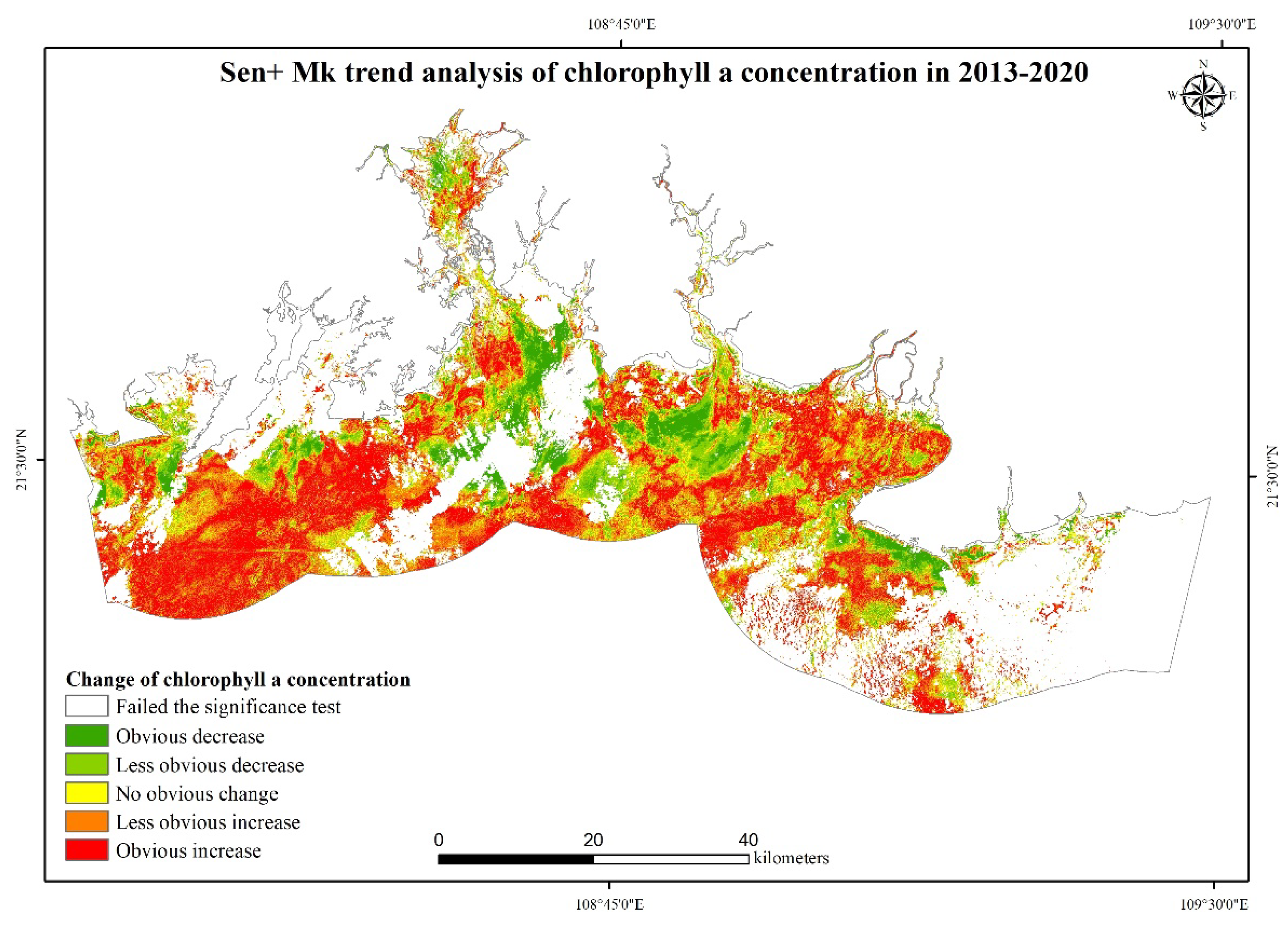
| Obvious decrease | 193.550 |
| Less obvious decrease | 356.720 |
| No obvious change | 383.690 |
| Less obvious increase | 724.450 |
| Obvious increase | 761.490 |
| Failed the significance test | 1721.900 |
| Model | Variables | MAE (μg/L) | MAPE (%) | RMSE (μg/L) | R2 |
|---|---|---|---|---|---|
| Single band | B3 | 3.381 | 65.758 | 3.705 | 0.563 |
| B4 | 3.006 | 58.470 | 2.903 | 0.719 | |
| Band ratio | B4/B1 | 1.967 | 38.261 | 1.935 | 0.706 |
| Band combination | B2 + B3 | 2.035 | 39.582 | 2.248 | 0.637 |
| B2 + B4 | 1.898 | 36.927 | 2.029 | 0.671 | |
| B3 + B4 | 1.795 | 34.913 | 1.959 | 0.698 | |
| Water index | FAI | 1.843 | 35.884 | 2.226 | 0.591 |
| SVM | B4, B3 + B4, B3, B1 − B4, B2 + B4, B1 + B4, B2 − B4 | 2.085 | 39.784 | 2.986 | 0.527 |
| GBDT model | B4, B3 + B4, B3, B1 − B4, B2 + B4, B1 + B4, B2 − B4 | 0.998 | 19.414 | 1.626 | 0.778 |
| Neural network | B4, B3 + B4, B3, B1 − B4, B2 + B4, B1 + B4, B2 − B4 | 1.492 | 28.472 | 1.974 | 0.714 |
| Date | Temperature | Wind Direction | Wind Strength |
|---|---|---|---|
| 14 April 2015 | 14.3 | SE | <3 |
| 23 October 2015 | 27.2 | S | <3 |
| 3 June 2016 | 31.2 | S | <3 |
| 28 December 2016 | 18 | N | 1 |
| 14 February 2017 | 17.44 | N | 1 |
| 2 March 2017 | 17.22 | SW | 1 |
| 28 October 2017 | 25.72 | N | 3–4 |
Publisher’s Note: MDPI stays neutral with regard to jurisdictional claims in published maps and institutional affiliations. |
© 2021 by the authors. Licensee MDPI, Basel, Switzerland. This article is an open access article distributed under the terms and conditions of the Creative Commons Attribution (CC BY) license (https://creativecommons.org/licenses/by/4.0/).
Share and Cite
Yao, H.; Huang, Y.; Wei, Y.; Zhong, W.; Wen, K. Retrieval of Chlorophyll-a Concentrations in the Coastal Waters of the Beibu Gulf in Guangxi Using a Gradient-Boosting Decision Tree Model. Appl. Sci. 2021, 11, 7855. https://doi.org/10.3390/app11177855
Yao H, Huang Y, Wei Y, Zhong W, Wen K. Retrieval of Chlorophyll-a Concentrations in the Coastal Waters of the Beibu Gulf in Guangxi Using a Gradient-Boosting Decision Tree Model. Applied Sciences. 2021; 11(17):7855. https://doi.org/10.3390/app11177855
Chicago/Turabian StyleYao, Huanmei, Yi Huang, Yiming Wei, Weiping Zhong, and Ke Wen. 2021. "Retrieval of Chlorophyll-a Concentrations in the Coastal Waters of the Beibu Gulf in Guangxi Using a Gradient-Boosting Decision Tree Model" Applied Sciences 11, no. 17: 7855. https://doi.org/10.3390/app11177855
APA StyleYao, H., Huang, Y., Wei, Y., Zhong, W., & Wen, K. (2021). Retrieval of Chlorophyll-a Concentrations in the Coastal Waters of the Beibu Gulf in Guangxi Using a Gradient-Boosting Decision Tree Model. Applied Sciences, 11(17), 7855. https://doi.org/10.3390/app11177855