
Performance Assessment of an Energy–Based Approximation Method for the Dynamic Capacity of RC Frames Subjected to Sudden Column Removal Scenarios


Abstract
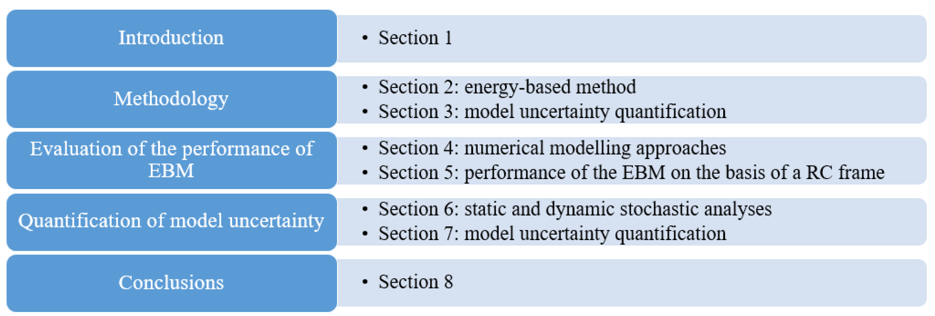
:1. Introduction
2. Energy–Based Method
- The moving sub–structure, subjected to a column failure, is assumed to behave like a single degree of freedom (SDOF) system [17,18,23]. The response is controlled by a single deformation mode and the mode keeps constant during the dynamic response. Therefore, the energy of the whole system can be linked to the energy of a point, i.e., every point in the system reaches its maximum displacement response at a same time. However, this never happens in a real structure as the existing infinite number of deformation modes will reach their maximum response at different moments. Consequently, the stored strain energy counted by the EBM is overestimated alongside its calculated deflections [23]. For a structural frame system subjected to an exterior column removal scenario, a non–single deformation response may occur due to complex load redistribution mechanisms (e.g., overturn), such as the results by [4,13,46] in relation to the exterior or side column removal scenarios.
- All the energy introduced into a system by the loads is switched into pure strain energy. The EBM neglects the energy dissipated by damping or other mechanisms. Therefore, the maximum deflection response will be overestimated. Moreover, it is still a controversial issue regarding how to model the damping mechanism for a sudden column removal scenario [19,47,48], e.g., viscous damping or Coulomb damping [23]. For instance, the studies have identified drawbacks associated with the use of Rayleigh damping based on initial stiffness, in which the initial stiffness may introduce in the unwanted artificial viscous forces [14,49]. This is because the stiffness term involved in the Rayleigh damping should also be updated accordingly when a system responds in the inelastic stage [48].
- The strain energy storage capacities of a system for a given displacement in static and dynamic situations are different [50]. The EBM cannot take this into account. However, the influence of the strain rate is low according to both previous experimental results [10] and numerical studies [19,23], as the maximum strain rates occur only in a small area and during a short time duration for sudden column removals.
3. Quantification of the Model Uncertainty Associated to the Application of EBM
- (a)
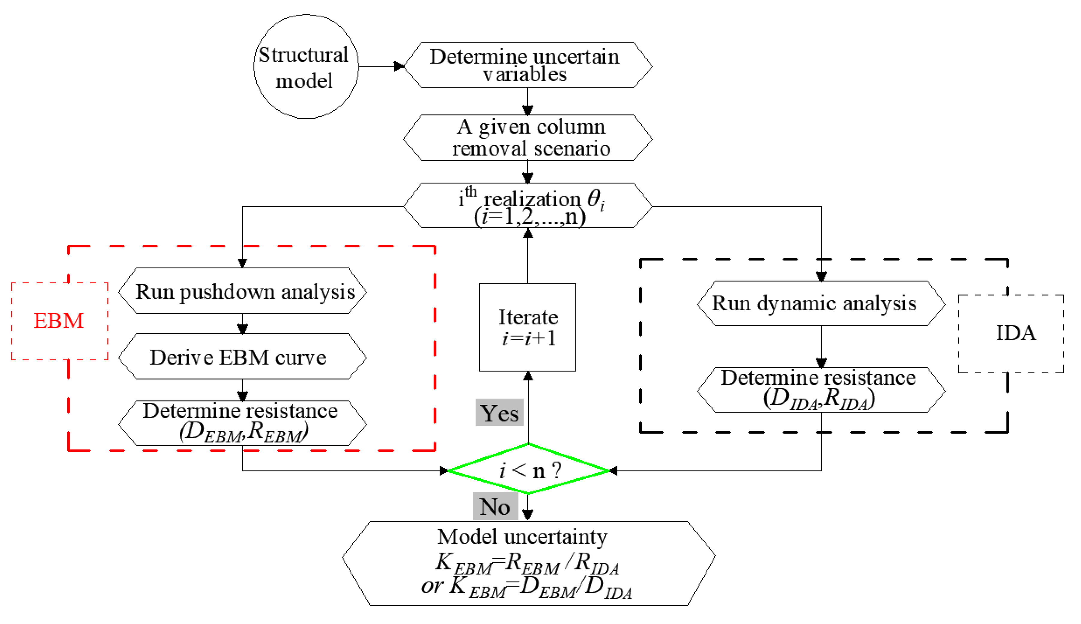
- Initially, the appropriate random variables and a column removal scenario are selected.
- (b)
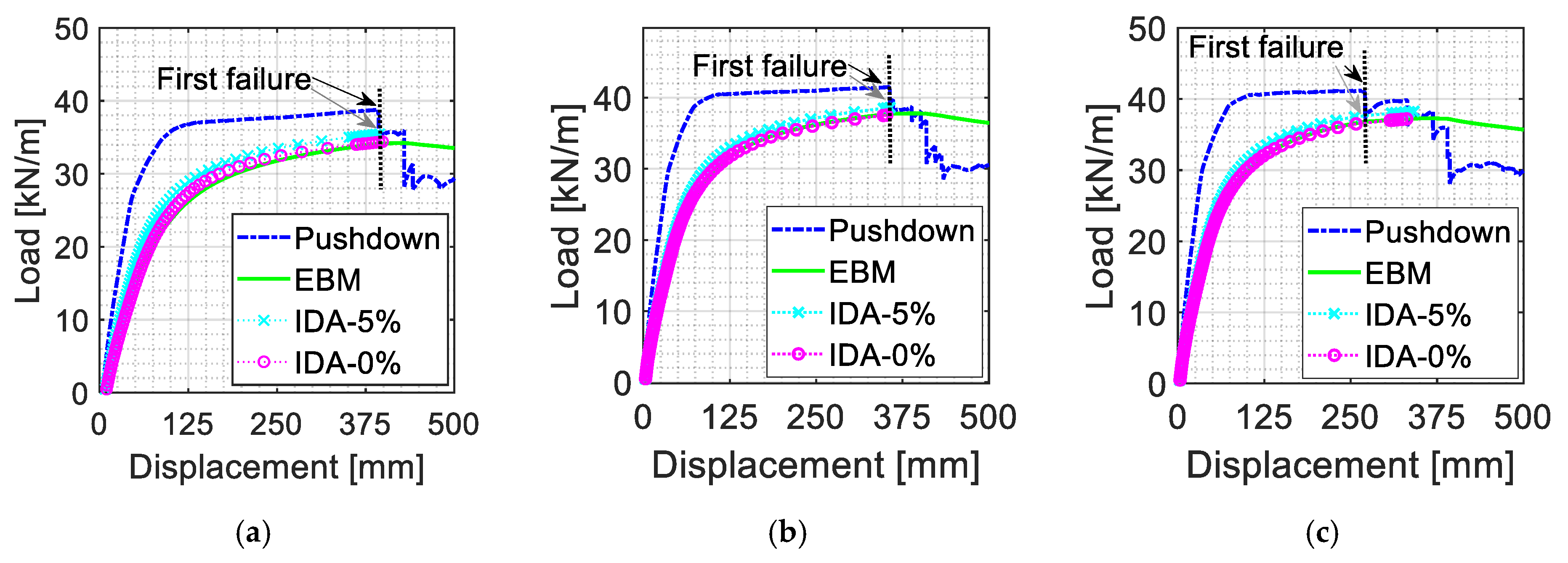
- Subsequently, both the non–linear static and dynamic analyses are carried out. In case of the former, the pushdown curve is subsequently used to derive the EBM curve and the corresponding dynamic resistance for every realization (the left branch in Figure 3). In case of the latter, incremental dynamic analyses (IDA) are executed to accurately determine the dynamic resistance for every realization (the right branch in Figure 3).
- (c)
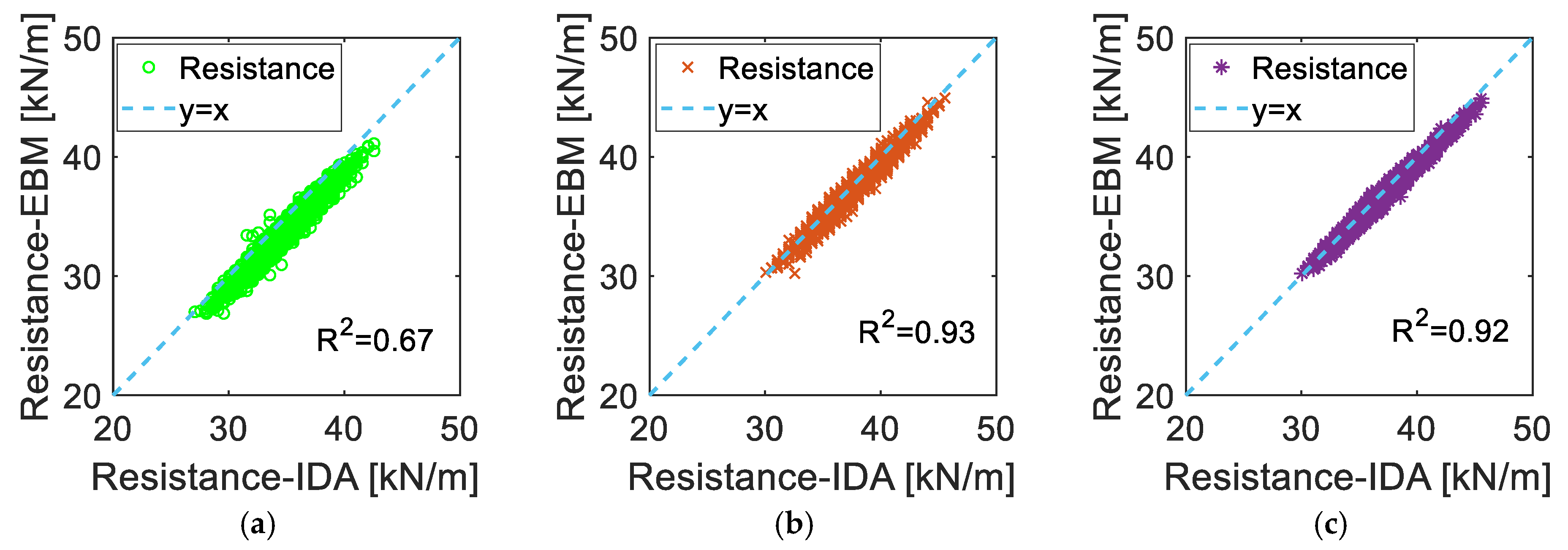
- Eventually, the model deviation for the EBM comparing to the IDA are calculated for both the resistances and the corresponding displacements:
4. Progressive Collapse Simulation Approaches for RC Structures
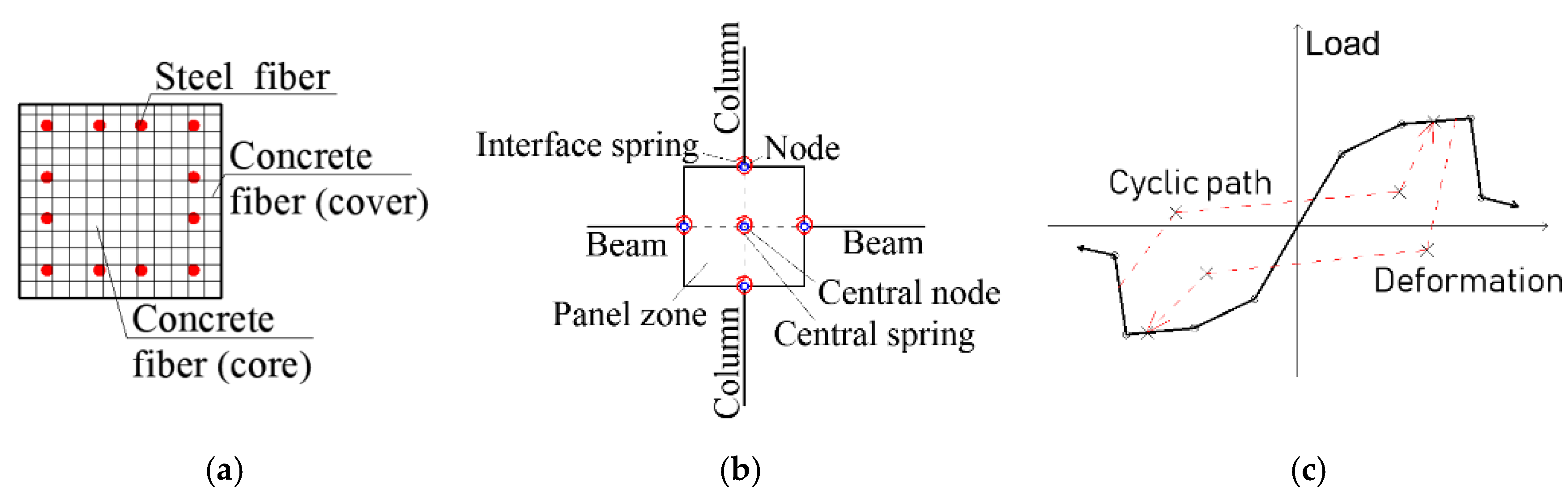
4.1. Finite Element Modelling
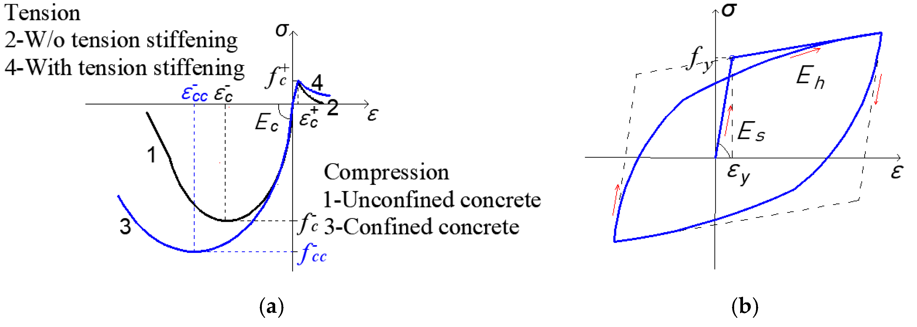
4.2. Material Models
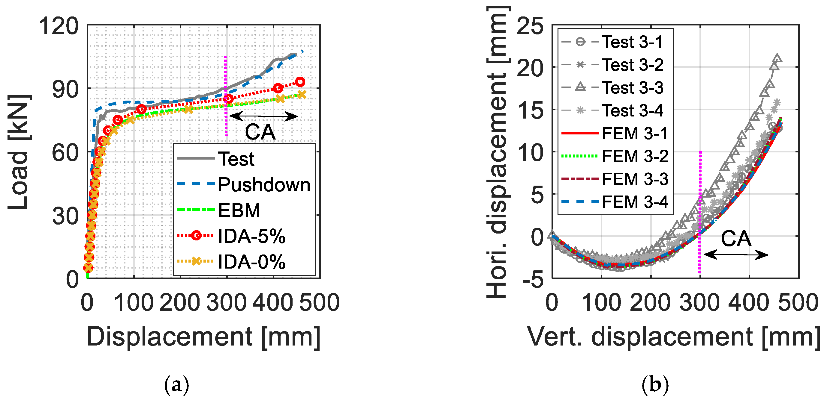
4.3. Validation of the Modelling Techniques
5. RC Frame Model Used for Model Uncertainty Quantification
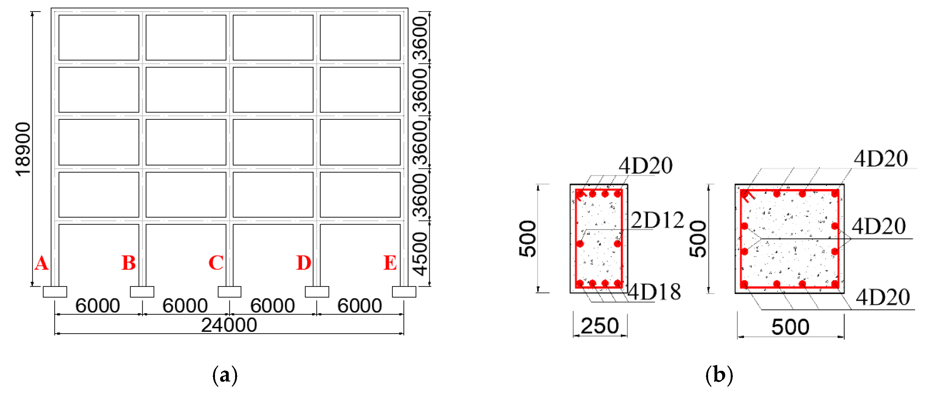
5.1. Description of the Structural Model
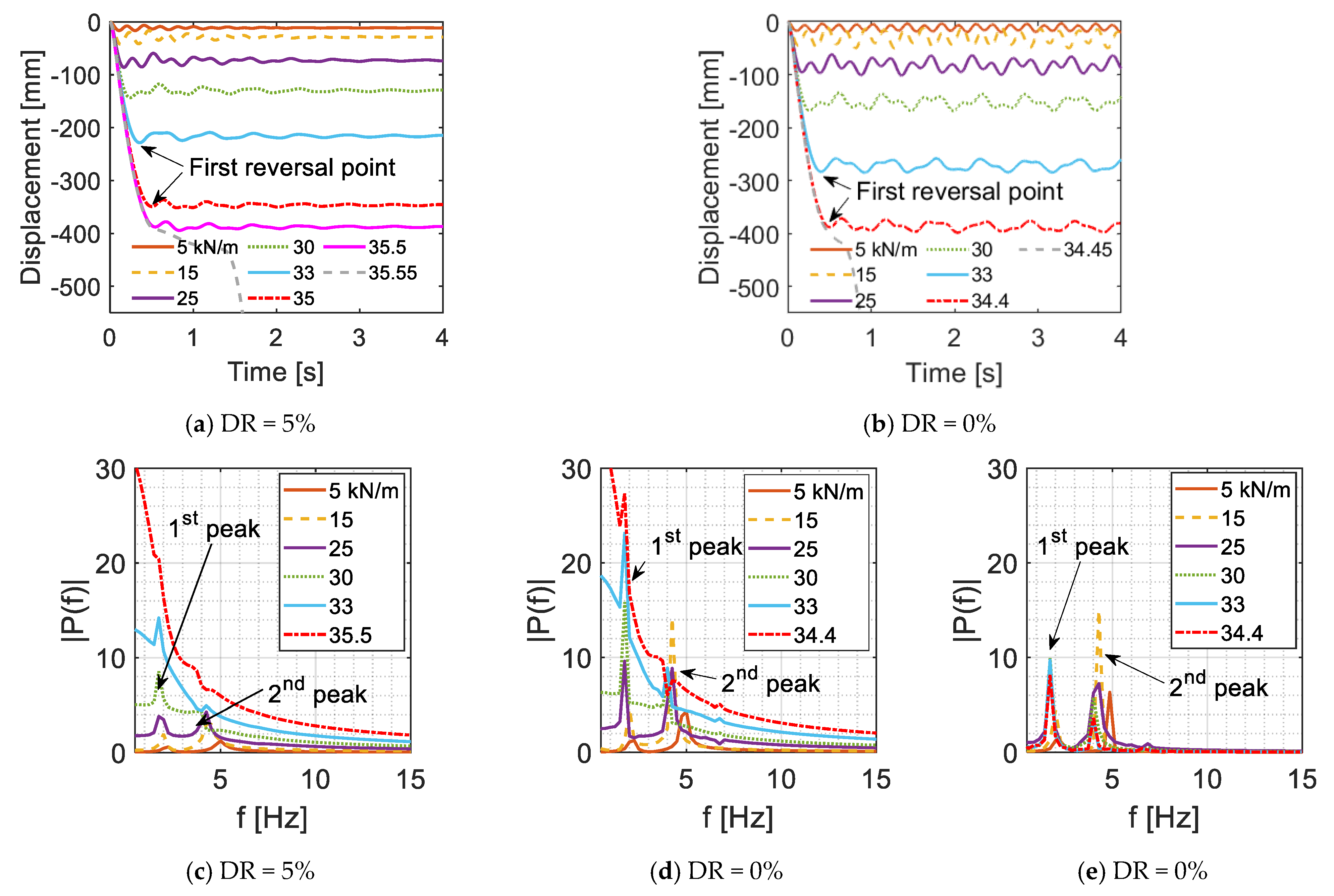
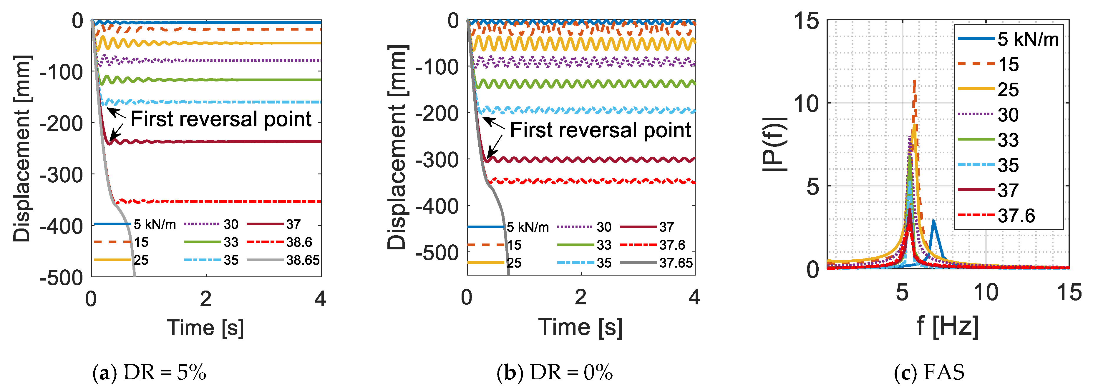
5.2. Dynamic Non–Linear Time History Analysis (NTHA)
5.3. Non–Linear Static Analysis
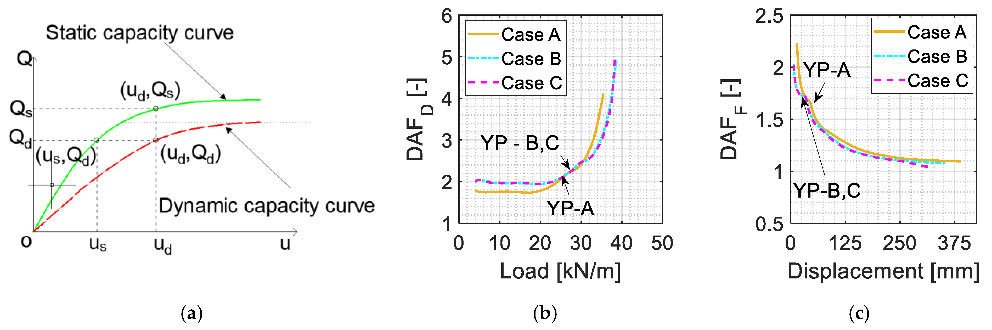
5.4. Dynamic Amplification Factor
5.5. Energy–Based Method
6. Stochastic Analysis
6.1. Probabilistic Models of Random Variables
6.2. Stochastic Analysis
7. Model Uncertainty Quantification of the EBM vs. IDA Analyses
- (1)
- Perform stochastic static non–linear analyses with specified random variables and column removal scenarios.
- (2)
- Apply the EBM (Equation (1)) to calculate dynamic ultimate capacities R according to the static capacity curves from step 1.
- (3)
- Evaluate the failure probability Pf through the following limit state function Z:
8. Conclusions
Author Contributions
Funding
Institutional Review Board Statement
Informed Consent Statement
Conflicts of Interest
References
- Adam, J.M.; Parisi, F.; Sagaseta, J.; Lu, X.Z. Research and practice on progressive collapse and robustness of building structures in the 21st century. Eng. Struct. 2018, 173, 122–149. [Google Scholar] [CrossRef]
- Botte, W.; Droogné, D.; Caspeele, R. Reliability-based resistance of RC element subjected to membrane action and their sensitivity to uncertainties. Eng. Struct. 2021, 238, 112259. [Google Scholar] [CrossRef]
- Parisi, F.; Scalvenzi, M. Progressive collapse assessment of gravity-load designed European RC buildings under multi-column loss scenarios. Eng. Struct. 2020, 209, 110001. [Google Scholar] [CrossRef]
- Parisi, F.; Scalvenzi, M.; Brunesi, E. Performance limit states for progressive collapse analysis of reinforced concrete framed buildings. Struct. Concr. 2019, 20, 68–84. [Google Scholar] [CrossRef] [Green Version]
- Zhang, L.; Li, H.H.; Wang, W. Retrofit Strategies against Progressive Collapse of Steel Gravity Frames. Appl. Sci. 2020, 10, 4600. [Google Scholar] [CrossRef]
- Droogné, D.; Botte, W.; Caspeele, R. A multilevel calculation scheme for risk-based robustness quantification of reinforced concrete frames. Eng. Struct. 2018, 160. [Google Scholar] [CrossRef]
- Faridmehr, I.; Baghban, M.H. An Overview of Progressive Collapse Behavior of Steel Beam-to-Column Connections. Appl. Sci. 2020, 10, 6003. [Google Scholar] [CrossRef]
- Qian, L.P.; Li, Y.; Diao, M.Z.; Guan, H.; Lu, X.Z. Experimental and Computational Assessments of Progressive Collapse Resistance of Reinforced Concrete Planar Frames Subjected to Penultimate Column Removal Scenario. J. Perform. Constr. Facil. 2020, 34, 04020019. [Google Scholar] [CrossRef]
- Adam, J.M.; Buitrago, M.; Bertolesi, E.; Sagaseta, J.; Moragues, J.J. Dynamic performance of a real-scale reinforced concrete building test under a corner-column failure scenario. Eng. Struct. 2020, 210, 110414. [Google Scholar] [CrossRef]
- Russell, J.M.; Owen, J.S.; Hajirasouliha, I. Experimental investigation on the dynamic response of RC flat slabs after a sudden column loss. Eng. Struct. 2015, 99, 28–41. [Google Scholar] [CrossRef]
- Qian, K.; Li, B. Investigation into Resilience of Precast Concrete Floors against Progressive Collapse. Aci Struct. J. 2019, 116, 171–182. [Google Scholar] [CrossRef]
- DoD. Design of Buildings to Resist Progressive Collapse. Unified Facilities Criteria (UFC) 4-023-03. 2016. Available online: https://www.wbdg.org/ffc/dod/unified-facilities-criteria-ufc/ufc-4-023-03 (accessed on 10 August 2021).
- Biagi, V.D.; Kiakojouri, F.; Chiaia, B.; Sheidaii, M.R. A Simplified Method for Assessing the Response of RC Frame Structures to Sudden Column Removal. Appl. Sci. 2020, 10, 3081. [Google Scholar] [CrossRef]
- Zheng, Z.; Tian, Y.; Yang, Z.B.; Lu, X.Z. Hybrid Framework for Simulating Building Collapse and Ruin Scenarios Using Finite Element Method and Physics Engine. Appl. Sci. 2020, 10, 4408. [Google Scholar] [CrossRef]
- Chen, X.X.; Xie, W.; Xiao, Y.F.; Chen, Y.G.; Li, X.J. Progressive Collapse Analysis of SRC Frame-RC Core Tube Hybrid Structure. Appl. Sci. 2018, 8, 2316. [Google Scholar] [CrossRef] [Green Version]
- Brunesi, E.; Nascimbene, R.; Parisi, F.; Augenti, N. Progressive collapse fragility of reinforced concrete framed structures through incremental dynamic analysis. Eng. Struct. 2015, 104, 65–79. [Google Scholar] [CrossRef]
- Xu, G.Q.; Ellingwood, B.R. An energy-based partial pushdown analysis procedure for assessment of disproportionate collapse potential. J. Constr. Steel Res. 2011, 67, 547–555. [Google Scholar] [CrossRef]
- Izzuddin, B.A.; Vlassis, A.G.; Elghazouli, A.Y.; Nethercot, D.A. Progressive collapse of multi-storey buildings due to sudden column loss—Part I: Simplified assessment framework. Eng. Struct. 2008, 30, 1308–1318. [Google Scholar] [CrossRef] [Green Version]
- Ding, L.; Van Coile, R.; Botte, W.; Caspeele, R. Quantification of model uncertainties of the energy-based method for dynamic column removal scenarios. Eng. Struct. 2021, 237, 112057. [Google Scholar] [CrossRef]
- Main, J.A. Composite Floor Systems under Column Loss: Collapse Resistance and Tie Force Requirements. J. Struct. Eng. 2014, 140, A4014003. [Google Scholar] [CrossRef] [Green Version]
- Yu, X.H.; Qian, K.; Lu, D.G.; Li, B. Progressive Collapse Behavior of Aging Reinforced Concrete Structures Considering Corrosion Effects. J. Perform. Constr. Facil. 2017, 31, 04017009. [Google Scholar] [CrossRef]
- Huang, M.; Huang, H.; Hao, R.; Chen, Z.; Li, M.; Deng, W. Studies on secondary progressive collapse-resistance mechanisms of reinforced concrete subassemblages. Struct. Concr. 2021. [Google Scholar] [CrossRef]
- Herraiz, B.; Vogel, T.; Russell, J. Energy-based method for sudden column failure scenarios: Theoretical, numerical and experimental analysis. In IABSE Workshop Helsinki 2015: Safety, Robustness and Condition Assessment of Structures; International Association for Bridge and Structural Engineering IABSE: Helsinki, Finland, 2015; pp. 70–77. [Google Scholar]
- Dusenberry, D.O.; Hamburger, R.O. Practical means for energy-based analyses of disproportionate collapse potential. J. Perform. Constr. Facil. 2006, 20, 336–348. [Google Scholar] [CrossRef]
- Liu, M.; Pirmoz, A. Energy-based pulldown analysis for assessing the progressive collapse potential of steel frame buildings. Eng. Struct. 2016, 123, 372–378. [Google Scholar] [CrossRef]
- Tsai, M.H.; Lin, B.H. Dynamic amplification factor for progressive collapse resistance analysis of an RC building. Struct. Des. Tall Spec. Build. 2009, 18, 539–557. [Google Scholar] [CrossRef]
- Ding, L.; Botte, W.; Van Coile, R.; Caspeele, R. Model Uncertainty Quantification for Column Removal Scenario Calculations Using the Energy-based Method. In Proceedings of the 13th FIB International PhD-Symposium in Civil Engineering, Paris, France, 26–28 August 2020. [Google Scholar]
- Ding, L.; Botte, W.; Van Coile, R.; Caspeele, R. Evaluation of the energy-based method for dynamic analysis under a sudden column removal scenario. In Proceedings of the FIB Symposium 2020: Concrete Structures for Resilient Society, Shanghai, China, 22–24 November 2020. [Google Scholar]
- Bao, Y.; Main, J.A.; Noh, S.Y. Evaluation of structural robustness against column loss: Methodology and application to RC frame buildings. J. Struct. Eng. 2017, 143, 04017066. [Google Scholar] [CrossRef] [Green Version]
- Ding, L.; Botte, W.; Van Coile, R.; Caspeele, R. Robustness-evaluation of a stochastic dynamic system and the instant equivalent extreme-value event: The PDEM-based structural reliability evaluation of a dynamic system. Beton Und Stahlbetonbau 2018, 113, 33–37. [Google Scholar] [CrossRef]
- Nagavedu Jayakumar, Y.; Kanchi, B.R. Probabilistic studies on mechanics-based shear capacity models for reinforced concrete beams with stirrups. Struct. Concr. 2020, 21, 376–392. [Google Scholar] [CrossRef]
- Gino, D.; Castaldo, P.; Giordano, L.; Mancini, G. Model uncertainty in non-linear numerical analyses of slender reinforced concrete members. Struct. Concr. 2021, 22, 845–870. [Google Scholar] [CrossRef]
- Botte, W.; Vereecken, E.; Taerwe, L.; Caspeele, R. Assessment of posttensioned concrete beams from the 1940s: Large-scale load testing, numerical analysis and Bayesian assessment of prestressing losses. Struct. Concr. 2021. [Google Scholar] [CrossRef]
- Biondini, F.; Frangopol, D.M. Time-variant redundancy and failure times of deteriorating concrete structures considering multiple limit states. Struct. Infrastruct. Eng. 2017, 13, 94–106. [Google Scholar] [CrossRef]
- Vereecken, E.; Botte, W.; Lombaert, G.; Caspeele, R. VoI-Based Optimization of Structural Assessment for Spatially Degrading RC Structures. Appl Sci. 2021, 11, 4994. [Google Scholar] [CrossRef]
- He, J.R.; Chen, J.B.; Ren, X.D.; Li, J. A shake table test study of reinforced concrete shear wall model structures exhibiting strong non-linear behaviors. Eng. Struct. 2020, 212, 110481. [Google Scholar] [CrossRef]
- Chen, J.B.; He, J.R.; Ren, X.D.; Li, J. Stochastic Harmonic Function Representation of Random Fields for Material Properties of Structures. J. Eng. Mech. 2018, 144, 04018049. [Google Scholar] [CrossRef]
- Thienpont, T.; Van Coile, R.; Caspeele, R.; De Corte, W. Burnout resistance of concrete slabs: Probabilistic assessment and global resistance factor calibration. Fire Saf. J. 2021, 119, 103242. [Google Scholar] [CrossRef]
- Jovanović, B.; Van Coile, R.; Hopkin, D.; Elhami Khorasani, N.; Lange, D.; Gernay, T. Review of current practice in probabilistic structural fire engineering: Permanent and live load modelling. Fire Technol. 2020. [Google Scholar] [CrossRef]
- Vereecken, E.; Botte, W.; Lombaert, G.; Caspeele, R. A Bayesian inference approach for the updating of spatially distributed corrosion model parameters based on heterogeneous measurement data. Struct. Infrastruct. Eng. 2020, 1–17. [Google Scholar] [CrossRef]
- Kamiński, M.; Świta, P. Structural stability and reliability of the underground steel tanks with the stochastic finite element method. Arch. Civ. Mech. Eng. 2015, 15, 593–602. [Google Scholar] [CrossRef]
- Bredow, R.; Kamiński, M. Computer analysis of dynamic reliability of some concrete beam structure exhibiting random damping. Int. J. Appl. Mech. Eng. 2021, 26. [Google Scholar] [CrossRef]
- Sørensen, J.D.; Rizzuto, E.; Narasimhan, H.; Faber, M.H. Robustness: Theoretical framework. Struct. Eng. Int. 2012, 22, 66–72. [Google Scholar] [CrossRef] [Green Version]
- Feng, D.; Xie, S.; Xu, J.; Qian, K. Robustness quantification of reinforced concrete structures subjected to progressive collapse via the probability density evolution method. Eng. Struct. 2020, 202, 109877. [Google Scholar] [CrossRef]
- JCSS. Risk Assessment in Engineering: Principles, System Representation and Risk Criteria; Narasimhan, H., Faber, M.H., Eds.; Joint Committee on Structural Safety (JCSS), 2009; Available online: https://www.jcss-lc.org/risk-assessment-in-engineering/ (accessed on 10 August 2021).
- Feng, D.; Wang, Z.; Wu, G. Progressive collapse performance analysis of precast reinforced concrete structures. Struct. Des. Tall Spec. Build. 2019, 28, e1588. [Google Scholar] [CrossRef]
- Wang, C.H.; Xiao, J.Z.; Liang, C.F. Study on nonlinear damping behavior of damaged recycled aggregate concrete beams. Struct. Concr. 2021. [Google Scholar] [CrossRef]
- Charney, F.A. Unintended consequences of modeling damping in structures. J. Struct. Eng. 2008, 134, 581–592. [Google Scholar] [CrossRef]
- Hall, J.F. Problems encountered from the use (or misuse) of Rayleigh damping. Earthq. Eng. Struct. Dyn. 2006, 35, 525–545. [Google Scholar] [CrossRef]
- Gao, X.; Zhou, L.; Ren, X.; Li, J. Rate effect on the stress–strain behavior of concrete under uniaxial tensile stress. Struct. Concr. 2020, 22, E815–E830. [Google Scholar] [CrossRef]
- Mazzoni, S.; McKenna, F.; Scott, M.H.; Fenves, G.L. OpenSees command language manual. Pac. Earthq. Eng. Res. (PEER) Cent. 2006, 264. [Google Scholar]
- Feng, D.; Ren, X. Implicit gradient-enhanced force-based Timoshenko fiber element formulation for reinforced concrete structures. Int. J. Numer. Methods Eng. 2020. [Google Scholar] [CrossRef]
- Ceresa, P.; Petrini, L.; Pinho, R. Flexure-Shear Fiber Beam-Column Elements for Modeling Frame Structures Under Seismic Loading—State of the Art. J. Earthq. Eng. 2007, 11, 46–88. [Google Scholar] [CrossRef]
- Vecchio, F.J.; Collins, M.P. The Modified Compression-Field Theory for Reinforced-Concrete Elements Subjected to Shear. J. Am. Concr. Inst. 1986, 83, 219–231. [Google Scholar]
- Lowes, L.N.; Altoontash, A. Modeling reinforced-concrete beam-column joints subjected to cyclic loading. J. Struct. Eng. 2003, 129, 1686–1697. [Google Scholar] [CrossRef]
- Wu, J.Y.; Li, J.; Faria, R. An energy release rate-based plastic-damage model for concrete. Int. J. Solids Struct. 2006, 43, 583–612. [Google Scholar] [CrossRef] [Green Version]
- Mander, J.B.; Priestley, M.J.N.; Park, R. Theoretical Stress-Strain Model for Confined Concrete. J. Struct. Eng. 1988, 114, 1804–1826. [Google Scholar] [CrossRef] [Green Version]
- Stevens, N.J.; Uzumeri, S.M.; Will, G.T. Constitutive model for reinforced concrete finite element analysis. Struct. J. 1991, 88, 49–59. [Google Scholar]
- Esmaeiltabar, P.; Vaseghi, J.; Khosravi, H. Nonlinear macro modeling of slender reinforced concrete shear walls. Struct. Concr. 2019, 20, 899–910. [Google Scholar] [CrossRef]
- Feng, D.; Kolay, C.; Ricles, J.M.; Li, J. Collapse simulation of reinforced concrete frame structures. Struct. Des. Tall Spec. Build. 2016, 25, 578–601. [Google Scholar] [CrossRef]
- fib. fib Model Code for Concrete Structures 2010; Ernst & Sohn, Wiley: Berlin, Germany, 2013. [Google Scholar] [CrossRef]
- Lu, X.; Lu, X.Z.; Guan, H.; Ye, L.P. Collapse simulation of reinforced concrete high-rise building induced by extreme earthquakes. Earthq. Eng. Struct. Dyn. 2013, 42, 705–723. [Google Scholar] [CrossRef] [Green Version]
- Yi, W.J.; He, Q.F.; Xiao, Y.; Kunnath, S.K. Experimental study on progressive collapse-resistant behavior of reinforced concrete frame structures. Aci Struct. J. 2008, 105, 433–439. [Google Scholar]
- CEN. Eurocode 2: Design of Concrete Structures—Part 1-1: General Rules and Rules for Buildings; British Standard Institution: London, UK, 2004. [Google Scholar]
- CEN. Eurocode 1: Actions on Structures-Part 1-1: General Actions-Densities, Self-Weight, Imposed Loads for Buildings; European Committee for Standardization: Brussel, Belgium, 2002. [Google Scholar]
- JCSS. Probabilistic model code. Jt. Comm. Struct. Saf. 2001. Available online: https://www.jcss-lc.org/jcss-probabilistic-model-code/ (accessed on 10 August 2021).
- Tsai, M.H.; Lin, B.H. Investigation of progressive collapse resistance and inelastic response for an earthquake-resistant RC building subjected to column failure. Eng. Struct. 2008, 30, 3619–3628. [Google Scholar] [CrossRef]
- Peng, Y.B.; Ding, L.C.; Chen, J.B. Performance evaluation of base-isolated structures with sliding hydromagnetic bearings. Struct. Control Health Monit. 2019, 26, e2278. [Google Scholar] [CrossRef] [Green Version]
- Peng, Y.B.; Ding, L.C.; Chen, J.B.; Liu, J.T.; Villaverde, R. Shaking Table Test of Seismic Isolated Structures with Sliding Hydromagnetic Bearings. J. Struct. Eng. 2020, 146, 04020174. [Google Scholar] [CrossRef]
- Lee, M.; Yoo, M.; Jung, H.S.; Kim, K.H.; Lee, I.W. Study on Dynamic Behavior of Bridge Pier by Impact Load Test Considering Scour. Appl. Sci. 2020, 10, 6741. [Google Scholar] [CrossRef]
- Tsai, M.H. An analytical methodology for the dynamic amplification factor in progressive collapse evaluation of building structures. Mech. Res. Commun. 2010, 37, 61–66. [Google Scholar] [CrossRef]
- Brunesi, E.; Nascimbene, R. Extreme response of reinforced concrete buildings through fiber force-based finite element analysis. Eng. Struct. 2014, 69, 206–215. [Google Scholar] [CrossRef]
- Holický, M.; Sýkora, M. Stochastic models in analysis of structural reliability. In Proceedings of the International Symposium on Stochastic Models in Reliability Engineering, Life Sciences and Operation Management, Beer Sheva, Israel, 8–11 February 2010. [Google Scholar]
- Olsson, A.; Sandberg, G.; Dahlblom, O. On Latin hypercube sampling for structural reliability analysis. Struct. Saf. 2003, 25, 47–68. [Google Scholar] [CrossRef]
- Arteta, C.A.; Piedrahita, J.; Ortiz, A.; Segura Jr, C.L.; Kolozvari, K. Quantifying the uncertainty in modeling of rc walls. In Proceedings of the 17th World Conference on Earthquake Engineering, Sendai, Japan, 13–18 September 2020. [Google Scholar]
- Astroza, R.; Alessandri, A. Effects of model uncertainty in nonlinear structural finite element model updating by numerical simulation of building structures. Struct. Control Health Monit. 2019, 26, e2297. [Google Scholar] [CrossRef]
- Kwon, O.-S.; Elnashai, A. The effect of material and ground motion uncertainty on the seismic vulnerability curves of RC structure. Eng. Struct. 2006, 28, 289–303. [Google Scholar] [CrossRef]
- Monteiro, R.; Delgado, R.; Pinho, R. Probabilistic Seismic Assessment of RC Bridges: Part I—Uncertainty Models. Structures 2016, 5, 258–273. [Google Scholar] [CrossRef]


| Material | Parameter | Units | Mean Value |
|---|---|---|---|
| Concrete | Compressive strength fc | MPa | 28 |
| Compressive peak strain ɛc1 | % | 0.21 | |
| Tensile strength fct | MPa | 2.2 | |
| Young’s modulus Eci | GPa | 30.3 | |
| Steel | Yield stress fy | MPa | 560 |
| Tensile strength fu | MPa | 655 | |
| Ultimate strain ɛu | % | 12 | |
| Young’s modulus Es | GPa | 205 |
| Case A | Case B | Case C | |
|---|---|---|---|
| RIDA–5% [kN/m] | 35.5 | 38.6 | 38.3 |
| RIDA–0% [kN/m] | 34.4 | 37.6 | 37.2 |
| Rpushdown [kN/m] | 38.8 | 41.5 | 41.2 |
| REBM [kN/m] | 34.1 | 37.7 | 36.8 |
| (REBM–RIDA–5%)/RIDA–5% | −3.94% | −2.33% | −3.92% |
| Variable | Units | Distribution | Mean | COV |
|---|---|---|---|---|
| c | mm | Beta | 30 | 0.17 |
| fc | MPa | Lognormal | 28 | 0.18 |
| ɛc1 | % | Lognormal | 0.21 | 0.15 |
| Y2,j | – | Lognormal | 1 | 0.30 |
| Es | GPa | Normal | 205 | 0.08 |
| fy | MPa | Lognormal | 560 | 0.05 |
| fu | MPa | Lognormal | 655 | 0.06 |
| ɛu | % | Lognormal | 12 | 0.15 |
| Case A | Case B | Case C | ||||
|---|---|---|---|---|---|---|
| Mean | St.D. | Mean | St.D. | Mean | St.D. | |
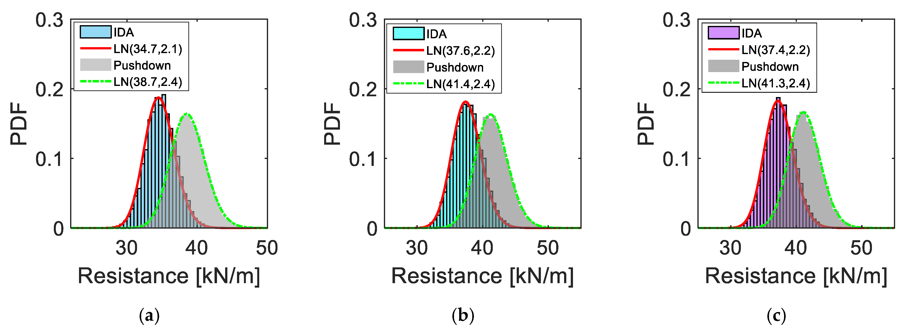
| RPushdown [kN/m] | 38.7 | 2.4 | 41.4 | 2.4 | 41.3 | 2.4 |
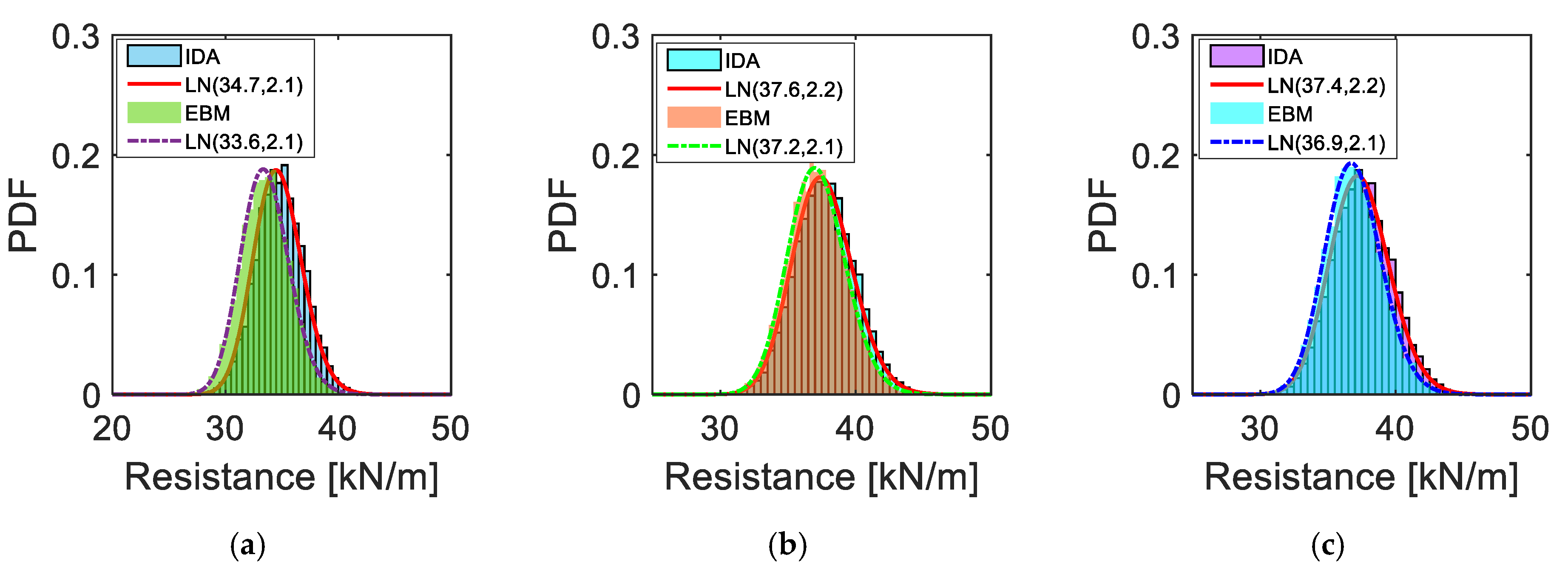
| RIDA [kN/m] | 34.7 | 2.1 | 37.6 | 2.2 | 37.4 | 2.2 |
| REBM [kN/m] | 33.6 | 2.1 | 37.2 | 2.1 | 36.9 | 2.1 |
| (REBM–RIDA)/RIDA | −3.17% | – | −1.06% | – | −1.34% | – |
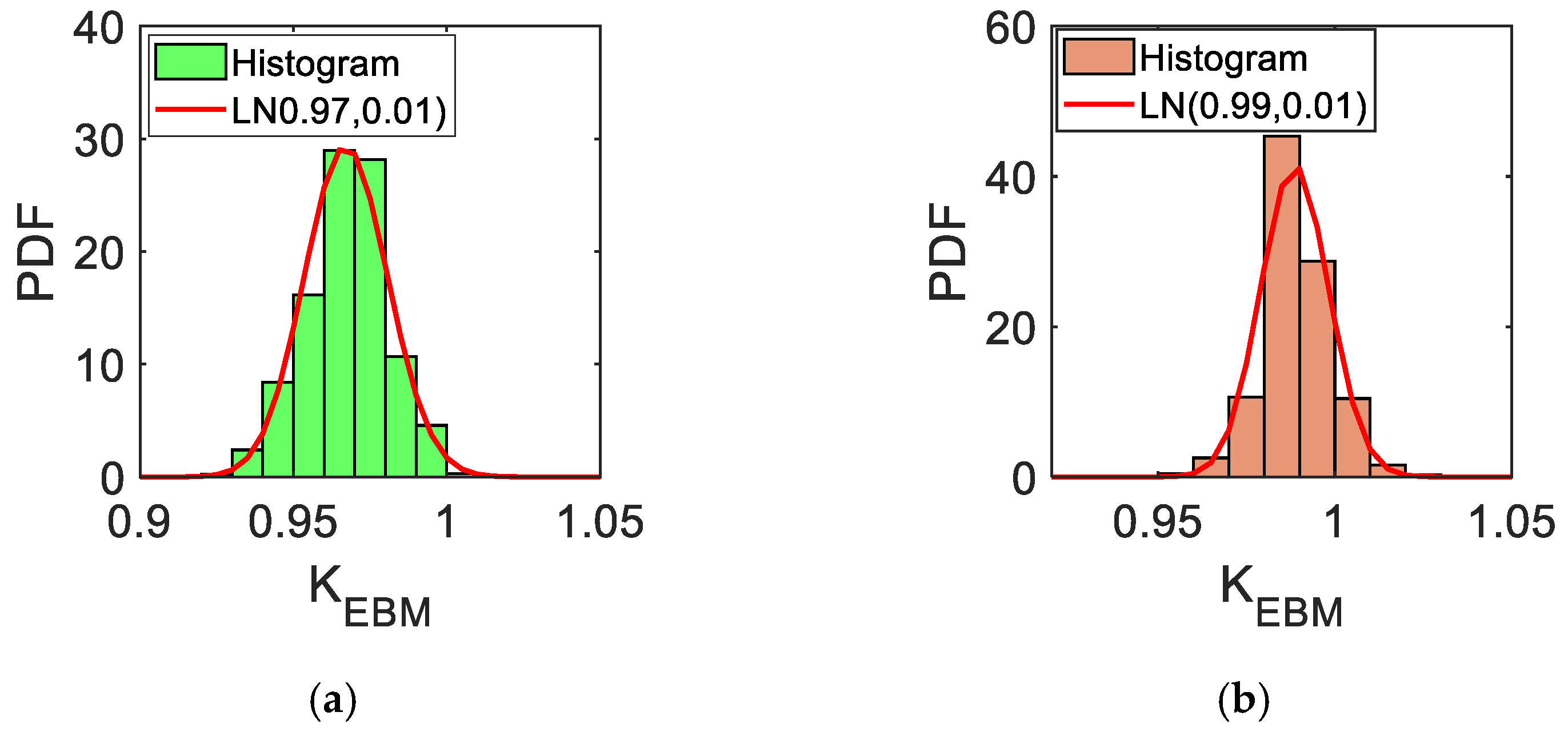
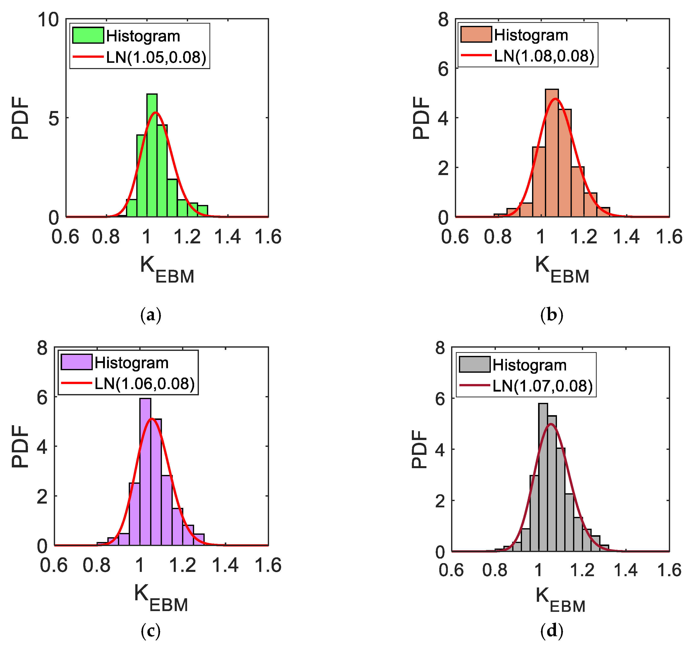
| Case | KEBM [–] | ||
|---|---|---|---|
| Mean (µ) | St.D. (σ) | ||
| Case A | 0.97 | 0.01 | |
| Case B | 0.99 | 0.01 | |
| Case C | 0.99 | 0.01 | |
| All | 0.98 | 0.02 | |
| Case A | 1.05 | 0.08 | |
| Case B | 1.08 | 0.08 | |
| Case C | 1.06 | 0.08 | |
| All | 1.07 | 0.08 | |
Publisher’s Note: MDPI stays neutral with regard to jurisdictional claims in published maps and institutional affiliations. |
© 2021 by the authors. Licensee MDPI, Basel, Switzerland. This article is an open access article distributed under the terms and conditions of the Creative Commons Attribution (CC BY) license (https://creativecommons.org/licenses/by/4.0/).
Share and Cite
Ding, L.; Van Coile, R.; Botte, W.; Caspeele, R. Performance Assessment of an Energy–Based Approximation Method for the Dynamic Capacity of RC Frames Subjected to Sudden Column Removal Scenarios. Appl. Sci. 2021, 11, 7492. https://doi.org/10.3390/app11167492
Ding L, Van Coile R, Botte W, Caspeele R. Performance Assessment of an Energy–Based Approximation Method for the Dynamic Capacity of RC Frames Subjected to Sudden Column Removal Scenarios. Applied Sciences. 2021; 11(16):7492. https://doi.org/10.3390/app11167492
Chicago/Turabian StyleDing, Luchuan, Ruben Van Coile, Wouter Botte, and Robby Caspeele. 2021. "Performance Assessment of an Energy–Based Approximation Method for the Dynamic Capacity of RC Frames Subjected to Sudden Column Removal Scenarios" Applied Sciences 11, no. 16: 7492. https://doi.org/10.3390/app11167492
APA StyleDing, L., Van Coile, R., Botte, W., & Caspeele, R. (2021). Performance Assessment of an Energy–Based Approximation Method for the Dynamic Capacity of RC Frames Subjected to Sudden Column Removal Scenarios. Applied Sciences, 11(16), 7492. https://doi.org/10.3390/app11167492