Full Explicit Numerical Modeling in Time-Domain for Nonlinear Electromagnetics Simulations in Ultrafast Laser Nanostructuring

Abstract

The purpose of this paper is to present a new and accurate, fully explicit finite-difference time-domain method for modeling nonlinear electromagnetics. The approach relies on a stable algorithm based on a general vector auxiliary differential equation in order to solve the curl Maxwell’s equation in a frequency-dependent and nonlinear medium. The energy conservation and stability of the presented scheme are theoretically proved. The algorithms presented here can accurately describe laser pulse interaction with metals and nonlinear dielectric media interfaces where Kerr and Raman effects, as well as multiphoton ionization and metal dispersion, occur simultaneously. The approach is finally illustrated by simulating the nonlinear propagation of an ultrafast laser pulse through a dielectric medium transiently turning to inhomogeneous metal-like states by local free-electron plasma formation. This free carrier generation can also be localized in the dielectric region surrounding nanovoids and embedded metallic nanoparticles, and may trigger collective effects depending on the distance between them. The proposed numerical approach can also be applied to deal with full-wave electromagnetic simulations of optical guided systems where nonlinear effects play an important role and cannot be neglected.

1. Introduction

The finite difference time-domain (FDTD) method enables the computation and modeling of light propagation and scattering processes in linear and nonlinear dispersive materials possessing wavelength-dependent and intensity-dependent properties. This ranks the method among the most universal and powerful numerical tools for optics, electrodynamics, antennas, and waveguides theory. In this context, the general vector auxiliary differential equation (GVADE) method, which has been reported in [1] and improved in [2], is one of the most popular methods to deal with nonlinear media. However, the method suffers from some drawbacks that limit its speed and stability due to the semi-implicit updating relation for the current polarization densities. In summary, the method is not appropriate or recommended for a broad range of problems, especially those that address the designs with complex 3D topology, where iterative solutions of coupled nonlinear equations can be unstable and resource-demanding [3]. Some direct or explicit methods take into consideration the Kerr effect in the Born–Oppenheimer approximation [4]. The Kerr effect arises from the nonlinear third-order electric susceptibility. In [3], the authors take into consideration the Kerr effect in an explicit form. Other direct methods [5] require excessive computational burdens, especially for the consideration of complex geometries. When metal–dielectric interfaces are treated, especially at nanometric scales, plasmonic effects appear [6,7] and generate high concentrations or high local densities of the electromagnetic field [8]. Since dielectrics experience nonlinear optical processes, the treatment of these regions in the interfaces is particularly challenging.

In this manuscript, we develop an algorithm that permits solving a nonlinear dielectric medium in which Kerr and Raman’s effects [9] occur simultaneously. The Raman effect arises from the scattering caused by the conversion of photon energies into vibrational energy of molecules. The scattered photons have less energy than the incident photons corresponding, therefore lowering frequency fields [2]. We also assume that this takes place in an inhomogeneous dielectric environment that can potentially include metallic heterogeneities with specific optical properties. Along with the laser propagation, provided that the intensity is sufficient to ensure nonlinear absorption, the medium can also turn into a metallic state as a free electron population is generated during multiphoton absorption (MPA) or tunneling and avalanche ionization processes. It is well known that the electron transition from the valence band (VB) to the conduction band (CB) is followed by various processes, including heating in the CB, impact ionization, and various kinds of electron collisions. The purpose of this work consists of computing all these events in a full explicit form. The carrier generation rate $G\left(\overrightarrow{r},t\right)$ has been computed owing to the BVkP approach implying Bloch–Volkov states [10]. The algorithms presented in this manuscript are especially suitable for simulations dealing with confinements and guiding high-energy pulsed beams. In summary, in this work, we coupled Maxwell equations and the electric charge carriers conservation equation in which the quantum ionization and recombination are governed by BVkP self-consistently.

In the next sections, by following and enriching some pioneers’ works [11,12,13], we detail a fully explicit, stable algorithm based on GVADE FDTD, able to solve the curl Maxwell’s equation in a frequency-dependent way for a nonlinear medium. In order to illustrate the combination of all these nonlinear effects occurring simultaneously in a simulation, we have modeled a Bessel beam traveling through dielectric fused silica, where some metal inclusions are modeled in a similar form as in Ref. [14]. In Section 2, we introduce the theoretical model, which describes the nonlinear effects. Section 3 presents the algorithms that discretize in time and space the main magnitudes, electromagnetic fields and electric charge. Appendix A is devoted to the stability condition assessment for these algorithms, which imposed numerical limits to the simulation performance. These limits are studied in Section 4, where we specify the validity framework considering natural limits imposed by physics. In Section 5 we present the simulation outcomes provided by the full numerical modelling and in Section 6 the conclusions are drawn. Finally, the stability conditions are derived in Appendix A and the used computational resources are presented in Appendix B.

2. Modeling Electromagnetic Fields in Nonlinear Media

The Equations (1)–(3) model the laser beam propagation by means of the electromagnetic fields $\overrightarrow{E}\left(\overrightarrow{r},t\right)$ and $\overrightarrow{H}\left(\overrightarrow{r},t\right)$. Throughout the light propagation path, fields generate and couple with the density of free charges as free electrons $n_{f{e}^{-}}\left(\overrightarrow{r},t\right)$, which in turn interact with the local field. In the given form, nonlinearities are determined by the electric displacement field $\overrightarrow{D}\left(\overrightarrow{r},t\right)$ in the Ampère-Maxwell Equation (1). Meanwhile, the evolution of the free-electron density or medium conductivity is described by Equation (3), where $G\left(\overrightarrow{r},t\right)$ is the carrier generation rate and $R\left(\overrightarrow{r},t\right)$ is the carrier recombination rate.

$$\begin{array}{ccc}\hfill \nabla \wedge \overrightarrow{H}\left(\overrightarrow{r},t\right)& =& \frac{\partial \overrightarrow{D}\left(\overrightarrow{r},t\right)}{\partial t}\hfill \end{array}$$

(1)

$$\begin{array}{ccc}\hfill \nabla \wedge \overrightarrow{E}\left(\overrightarrow{r},t\right)& =& -\mu \frac{\partial \overrightarrow{H}\left(\overrightarrow{r},t\right)}{\partial t}\hfill \end{array}$$

(2)

$$\begin{array}{ccc}\hfill \frac{\partial n_{f{e}^{-}}\left(\overrightarrow{r},t\right)}{\partial t}& =& G\left(\overrightarrow{r},t\right)-R\left(\overrightarrow{r},t\right)\hfill \end{array}$$

(3)

The electric displacement field is composed by the electric field contribution plus the polarization vectors $\overrightarrow{D}\left(\overrightarrow{r},t\right)={\epsilon }_0{\epsilon }_{\infty }\overrightarrow{E}\left(\overrightarrow{r},t\right)+\sum \overrightarrow{P}\left(\overrightarrow{r},t\right)$ [2]. The magnitude ${\epsilon }_{\infty }$ is the non-unity high-frequency relative permittivity of the media. On the right hand side of the displacement electric field, the sum of polarization vectors in the model that we are considering $\sum \overrightarrow{P}\left(\overrightarrow{r},t\right)$ is the contribution of four terms, the metal polarization ${\overrightarrow{P}}_{Metal}\left(\overrightarrow{r},t\right)$, the Kerr effect polarization ${\overrightarrow{P}}_{Kerr}\left(\overrightarrow{r},t\right)$, the Raman polarization ${\overrightarrow{P}}_{Raman}\left(\overrightarrow{r},t\right)$ and the free charge polarization vector ${\overrightarrow{P}}_{f{e}^{-}}\left(\overrightarrow{r},t\right)$ such as $\sum \overrightarrow{P}\left(\overrightarrow{r},t\right)={\overrightarrow{P}}_{Metal}\left(\overrightarrow{r},t\right)+{\overrightarrow{P}}_{Kerr}\left(\overrightarrow{r},t\right)+{\overrightarrow{P}}_{Raman}\left(\overrightarrow{r},t\right)+{\overrightarrow{P}}_{f{e}^{-}}\left(\overrightarrow{r},t\right)$ with the detail of each term below:

$$\begin{array}{ccc}\hfill {\overrightarrow{P}}_{Metal}\left(\overrightarrow{r},t\right)& =& \frac{{ϵ}_{0}a}{j\omega +b}\overrightarrow{E}\left(\overrightarrow{r},t\right)a,b\in \mathbb{C}\hfill \end{array}$$

(4)

$$\begin{array}{ccc}\hfill {\overrightarrow{P}}_{Kerr}\left(\overrightarrow{r},t\right)& =& \alpha {ϵ}_0{\chi }_0^{\left(3\right)}\overrightarrow{E}\left(\overrightarrow{r},t\right){\int }_{-\infty }^t\delta (t-\tau ){|\overrightarrow{E}(\overrightarrow{r},\tau )|}^{2}d\tau \hfill \end{array}$$

(5)

$$\begin{array}{ccc}\hfill {\overrightarrow{P}}_{Raman}\left(\overrightarrow{r},t\right)& =& \Psi \overrightarrow{E}\left(\overrightarrow{r},t\right){\int }_{-\infty }^t{e}^{\frac{-(t-\tau )}{{\tau }_2}}sin\left(\frac{t-\tau }{{\tau }_1}\right)U(t-\tau ){|\overrightarrow{E}(\overrightarrow{r},\tau )|}^{2}d\tau \hfill \end{array}$$

(6)

$$\begin{array}{ccc}\hfill {\overrightarrow{P}}_{f{e}^{-}}\left(\overrightarrow{r},t\right)& =& {\int }_{-\infty }^t{\sigma }_{f{e}^{-}}\left(\overrightarrow{r},t\right)\overrightarrow{E}\left(\overrightarrow{r},t\right)d\tau \hfill \end{array}$$

(7)

where $\Psi ={\epsilon }_0{\chi }^{\left(3\right)}(1-\alpha )\frac{{\tau }_1^2+{\tau }_2^2}{{\tau }_1{\tau }_2^{b}yte,intent\left(in\right)::types2}$ is a coefficient gathering parameters depending on the considered medium. Expressions Equations (5) and (6) providing the Kerr effect polarization and Raman polarization, respectively, are taken from [9]. Here, $\alpha$ is a real-valued constant in the range $\alpha \in [0,1]$ that parameterizes the relative strengths of Kerr and Raman contributions, $\delta \left(t\right)$ refers to the Dirac delta function that models the Kerr nonresonant virtual electronic transitions, which is medium dependent and in the order of few femtoseconds for fused silica, $U\left(t\right)$ is the Heaviside unit step function, $e^{\frac{-t}{{\tau }_2}}sin(\frac{t}{{\tau }_1})$ models the impulse response of a single Lorentzian relaxation centered on the optical phonon frequency $1/{\tau }_1$ and having a bandwidth of $1/{\tau }_2$. Finally ${\chi }_0^{\left(3\right)}$ is the strength of the third-order nonlinear electric susceptibility.

The upper limit of the integrations in Equations (5)–(7) extends only up to t because the response function must be zero for $\tau >t$ to ensure causality [3]. Moreover, free-charge polarization is introduced by using a free-charge density of current, which will be defined later. Finally, to model the metal, we consider a complex electrical permittivity $\widetilde{ϵ}\left(\omega \right)=\frac{a}{j\omega +b}$ where a and b are complex numbers that fit experimental data [15]. To model the dispersive media, we assume an electric permittivity, which is frequency-dependent as the calculations are devoted to ultrafast laser propagation, with bandwidth-limited pulses that exhibit wavelength dispersion.

In ref. [2], the general vector auxiliary differential equation technique allows considering nonlinearities or dispersive characteristics of a medium. They are introduced into the Ampère–Maxwell equation by means of current densities. These currents correspond intrinsically to the temporal variation of the polarization vectors. Thereby, the following Equations (8)–(11) can be derived to correlate the currents ${\overrightarrow{J}}_{Metal}\left(\overrightarrow{r},t\right)=\frac{\partial {\overrightarrow{P}}_{Metal}\left(\overrightarrow{r},t\right)}{\partial t}$, ${\overrightarrow{J}}_{Kerr}\left(\overrightarrow{r},t\right)=\frac{\partial {\overrightarrow{P}}_{Kerr}\left(\overrightarrow{r},t\right)}{\partial t}$, ${\overrightarrow{J}}_{Raman}\left(\overrightarrow{r},t\right)=\frac{\partial {\overrightarrow{P}}_{Raman}\left(\overrightarrow{r},t\right)}{\partial t}$, ${\overrightarrow{J}}_{f{e}^{-}}\left(\overrightarrow{r},t\right)=\frac{\partial {\overrightarrow{P}}_{f{e}^{-}}\left(\overrightarrow{r},t\right)}{\partial t}$ with the electric field:

$$\begin{array}{ccc}\hfill {\overrightarrow{J}}_{Metal}\left(\overrightarrow{r},t\right)& =& \frac{a{ϵ}_0}{b}\frac{\overrightarrow{E}\left(\overrightarrow{r},t\right)}{\partial t}-\frac{1}{b}\frac{{\overrightarrow{J}}_{Metal}\left(\overrightarrow{r},t\right)}{\partial t}\hfill \end{array}$$

(8)

$$\begin{array}{ccc}\hfill {\overrightarrow{J}}_{Kerr}\left(\overrightarrow{r},t\right)& =& {\displaystyle \alpha {ϵ}_0{\chi }_0^{\left(3\right)}\frac{\partial }{\partial t}\left[\overrightarrow{E}\left(\overrightarrow{r},t\right){\int }_0^t\delta (t-\tau ){|\overrightarrow{E}(\overrightarrow{r},\tau )|}^{2}d\tau \right]}\hfill \end{array}$$

(9)

$$\begin{array}{ccc}\hfill {\overrightarrow{J}}_{Raman}\left(\overrightarrow{r},t\right)& =& {\displaystyle \Psi \frac{\partial }{\partial t}\left[\overrightarrow{E}\left(\overrightarrow{r},t\right){\int }_0^t{e}^{\frac{-(t-\tau )}{{\tau }_2}}sin\left(\frac{t-\tau }{{\tau }_1}\right)U(t-\tau ){|\overrightarrow{E}(\overrightarrow{r},\tau )|}^{2}d\tau \right]}\hfill \end{array}$$

(10)

$$\begin{array}{ccc}\hfill {\overrightarrow{J}}_{f{e}^{-}}\left(\overrightarrow{r},t\right)& =& {\sigma }_{f{e}^{-}}\left(\overrightarrow{r},t\right)\overrightarrow{E}\left(\overrightarrow{r},t\right)\hfill \end{array}$$

(11)

We define a free-charge density of current as an Ohmic current, where the conductivity ${\sigma }_{f{e}^{-}}\left(\overrightarrow{r},t\right)=q{\mu }_{f{e}^{-}}{n}_{f{e}^{-}}\left(\overrightarrow{r},t\right)$ is given by the following frequency dependent expression:

$$\begin{array}{c}\hfill \sigma \left(\overrightarrow{r},\omega \right)=\frac{q{\mu }_{f{e}^{-}}{f}_d(|\overrightarrow{E}|)n_{ph-e^{-}}(|\overrightarrow{E}|)}{j\omega +f_r(|\overrightarrow{E}|)-f_a(|\overrightarrow{E}|)-f_{\eta }(|\overrightarrow{E}|)}\end{array}$$

(12)

where q is the electron charge, ${\mu }_{f{e}^{-}}$ the free carriers of charge mobility, $n_{f{e}^{-}}\left(\overrightarrow{r},t\right)$ the free-charge density and $n_{ph-e^{-}}\left(\overrightarrow{r},t\right)$ the photo-ionized electron density. This definition for the density of current Equation (11) is similar to Equation (9) in [10]. In Equation (13), we employ free-charge which is governed by Equation (3), or generation Equation (13) and recombination Equation (14) rates. In [10], the authors explain that electron density $n_{ph-e^{-}}\left(\overrightarrow{r},t\right)$ produced in the conduction band only describes the interaction of an electron with the laser electric field and accounts for the lattice periodicity, but does not account for possible collisions with phonons, ions, or other electrons. Due to these collisions, the coherence between the excited electron to the CB and its parent ion is destroyed and may introduce deviations from the above-predicted evolution of the electron density in the CB with respect to time. Indeed, without collisions, the produced electron density was shown to oscillate with time as a conduction electron may go back and forth to the VB through the action of the electromagnetic field [10,16]. Obviously, in an oscillation, the energy stays constant [17]. Hence, the authors of [10] defined a free state as a state where the electrons can be heated by inverse bremsstrahlung (IB) and are decorrelated from the parent ion. The density of charge associated with this free state is called here density of free-charge $n_{f{e}^{-}}\left(\overrightarrow{r},t\right)$, and its evolution along the time is modeled by Equation (3). Nevertheless, the ${\mu }_{f{e}^{-}}$, the free carriers of charge mobility, then we employ experimental data, which allow the determination of this parameter. The method is explained in detail in Section 5.

$$\begin{array}{ccc}\hfill G\left(\overrightarrow{r},t\right)& =& f_d\left(\overrightarrow{r},t\right)n_{ph-e^{-}}\left(\overrightarrow{r},t\right)+n_{f{e}^{-}}\left(\overrightarrow{r},t\right)\left[f_a\left(\overrightarrow{r},t\right)+f_{\eta }\left(\overrightarrow{r},t\right)\right]\hfill \end{array}$$

(13)

$$\begin{array}{ccc}\hfill R\left(\overrightarrow{r},t\right)& =& f_r\left(\overrightarrow{r},t\right)n_{f{e}^{-}}\left(\overrightarrow{r},t\right)\hfill \end{array}$$

(14)

In the carrier generation rate, the term associated with the photo-ionized electron density $n_{ph-e^{-}}\left(\overrightarrow{r},t\right)$ produced in the conduction band is a function of $|\overrightarrow{E}\left(\overrightarrow{r},t\right)|$. From Equation (5) in [10] we know that $\frac{\partial }{\partial t}\left[n_{ph-e^{-}}\left(\overrightarrow{r},t\right)-N_0\sum _c{\left|T_{cv}\left(t\right)\right|}^2\right]=0$ and hence $n_{ph-e^{-}}\left(\overrightarrow{r},t\right)-N_0\sum _c{\left|T_{cv}\left(t\right)\right|}^2=cte$. If this constant $cte=0$, then $n_{ph-e^{-}}\left(\overrightarrow{r},t\right)=0$ when $\overrightarrow{E}\left(\overrightarrow{r},t\right)=\overline{0}$. Combining this result with Equations (3) and (4) in [10], we calculate $n_{ph-e^{-}}\left(\overrightarrow{r},t\right)$ by Equation (15).

$$\begin{array}{c}\hfill n_{ph-e^{-}}\left(\overrightarrow{r},t\right)=\sum _{{\xi }_i=0}^{W_f}{\left|\frac{-\sqrt{E_g}{\int }_0^t\frac{|\overrightarrow{E}(\overrightarrow{r},\vartheta )|e^{-j\vartheta (E_g+{\xi }_i)}}{{\left(1-\frac{j}{\mathsf{\Omega }}{\int }_0^{\vartheta }|\overrightarrow{E}(\overrightarrow{r},\varrho )|d\varrho \right)}^2}d\vartheta }{N_0^{-1}(E_g+{\xi }_i)\sqrt{2m_{vc}^{*}}}\right|}^2\end{array}$$

(15)

Finally the functions related to the generation by ionization $f_d\left(\overrightarrow{r},t\right)$, impact $f_{\eta }\left(\overrightarrow{r},t\right)$ and avalanche $f_a\left(\overrightarrow{r},t\right)$, as well as the function related to the recombination of the free-charge $f_r\left(\overrightarrow{r},t\right)$, are given by the Equations (16)–(19), respectively.

$$\begin{array}{ccc}\hfill f_d\left(\overrightarrow{r},t\right)& =& \left\{\begin{array}{cc}\frac{1}{{\tau }_d}\hfill & \mathrm{if}|\overrightarrow{E}\left(\overrightarrow{r},t\right)|\ge \frac{E_{max}}{20}\hfill \\ \frac{20|\overrightarrow{E}\left(\overrightarrow{r},t\right)|}{{\tau }_d{E}_{max}}\hfill & \mathrm{if}|\overrightarrow{E}\left(\overrightarrow{r},t\right)|<\frac{E_{max}}{20}\hfill \end{array}\right.\hfill \end{array}$$

(16)

$$\begin{array}{ccc}\hfill f_{\eta }\left(\overrightarrow{r},t\right)& =& \left\{\begin{array}{cc}\eta \hfill & \mathrm{if}|\overrightarrow{E}\left(\overrightarrow{r},t\right)|\ge \frac{E_{max}}{20}\hfill \\ \frac{20|\overrightarrow{E}\left(\overrightarrow{r},t\right)|\eta }{E_{max}}\hfill & \mathrm{if}|\overrightarrow{E}\left(\overrightarrow{r},t\right)|<\frac{E_{max}}{20}\hfill \end{array}\right.\hfill \end{array}$$

(17)

$$\begin{array}{ccc}\hfill f_a\left(\overrightarrow{r},t\right)& =& \left\{\begin{array}{cc}\frac{\Theta |\overrightarrow{E}\left(\overrightarrow{r},t\right){|}^2}{\zeta }\hfill & \mathrm{Harmonic}\mathrm{field}\hfill \\ \Theta \left(\overrightarrow{E}\left(\overrightarrow{r},t\right)\wedge \overrightarrow{H}\left(\overrightarrow{r},t\right)\right)·\widehat{z}\hfill & \mathrm{No}\mathrm{harmonic}\mathrm{field}\hfill \end{array}\right.\hfill \end{array}$$

(18)

$$\begin{array}{ccc}\hfill f_r\left(\overrightarrow{r},t\right)& =& \left\{\begin{array}{cc}\frac{1}{{\tau }_r}\hfill & \mathrm{if}|\overrightarrow{E}\left(\overrightarrow{r},t\right)|\ge \frac{E_{max}}{20}\hfill \\ \frac{20|\overrightarrow{E}\left(\overrightarrow{r},t\right)|}{{\tau }_r{E}_{max}}\hfill & \mathrm{if}|\overrightarrow{E}\left(\overrightarrow{r},t\right)|<\frac{E_{max}}{20}\hfill \end{array}\right.\hfill \end{array}$$

(19)

In Equations (16)–(19), we find that the factor of maximum electric field reduction, which is suggested twenty times by [10], is taken into consideration. Nevertheless, when the photoionization process is considered in a truncated region where the magnitude of $|\overrightarrow{E}\left(\overrightarrow{r},t\right)|$ is from the beginning higher than the threshold $\frac{E_{max}}{20}$ reference value, these logical conditions can be suppressed in the nested loops, and this increases the algorithm performance. In other words, this simplification is possible when we assume the description with nonlinear effects in a particular region of the computational domain. So, the electromagnetic field that arrives at that region has a magnitude higher than the threshold $\frac{E_{max}}{20}$.

In Equation (18), we assume that $\frac{|\overrightarrow{E}\left(\overrightarrow{r},t\right){|}^2}{\zeta }$ is the fluence with $\zeta$ being the medium impedance. However, this is a particular case only valid when the electromagnetic field is a harmonic function in time. In general, and assuming a propagation along the z-axis, the power per surface is given by the Poynting vector.

3. Algorithms

The polarization vector due to the Kerr effect at the time $t={\Delta }_t\left(s-\frac{1}{2}\right)$ can be written as ${\overrightarrow{P}}_{Kerr}^{s-\frac{1}{2}}=\alpha {ϵ}_0{\chi }_0^{\left(3\right)}{|{\overrightarrow{E}}^{s-\frac{1}{2}}|}^2{\overrightarrow{E}}^{s-\frac{1}{2}}$; however, afterwards, at the instant ${\Delta }_t\left(s+\frac{1}{2}\right)$, in order to define a full explicit approach, we have to make the approximation ${\int }_0^{\left(s+\frac{1}{2}\right){\Delta }_t}\delta (t-\tau )|\overrightarrow{E}(\overrightarrow{r},\tau )|d\tau \simeq {\int }_0^{\left(s-\frac{1}{2}\right){\Delta }_t}\delta (t-\tau )|\overrightarrow{E}(\overrightarrow{r},\tau )|d\tau$. This approximation was demonstrated in [3] and leads to:

$$\begin{array}{c}\hfill {\overrightarrow{P}}_{Kerr}^{s+\frac{1}{2}}\simeq \alpha {ϵ}_0{\chi }_0^{\left(3\right)}{\overrightarrow{E}}^{s+\frac{1}{2}}{\int }_0^{\left(s-\frac{1}{2}\right){\Delta }_t}\delta (t-\tau )|\overrightarrow{E}(\overrightarrow{r},\tau )|d\tau \end{array}$$

This approximation ${\overrightarrow{P}}_{Kerr}^{s+\frac{1}{2}}\simeq \alpha {ϵ}_0{\chi }_0^{\left(3\right)}{|{\overrightarrow{E}}^{s-\frac{1}{2}}|}^2{\overrightarrow{E}}^{s+\frac{1}{2}}$ is valid under particular physical conditions explained in Section 4. To compute the nonlinear Raman effect, we make an analogous approximation. Considering that in this case there is no instantaneous cause–effect relationship, it is evident that the approximation is justified [18]. Therefore, by defining the scalar magnitude $|{\overrightarrow{Q}}_a\left(\overrightarrow{r},t\right)|$ that is defined from the vector ${\overrightarrow{Q}}_a\left(\overrightarrow{r},t\right)$, which could be considered as an instantaneous anisotropic Raman conductivity, we can discretize the Raman polarization vectors at the instants ${\Delta }_t\left(s-\frac{1}{2}\right)$ and ${\Delta }_t\left(s+\frac{1}{2}\right)$ as follows: ${\overrightarrow{P}}_{Raman}^{s-\frac{1}{2}}=|{\overrightarrow{Q}}_a^{s-\frac{1}{2}}|{\overrightarrow{E}}^{s-\frac{1}{2}}$ and ${\overrightarrow{P}}_{Raman}^{s+\frac{1}{2}}=|{\overrightarrow{Q}}_a^{s-\frac{1}{2}}|{\overrightarrow{E}}^{s+\frac{1}{2}}$. Where $|{\overrightarrow{Q}}_a^{s+\frac{1}{2}}|$ is updated from $|{\overrightarrow{Q}}_a^{s-\frac{1}{2}}|$ by means of:

$$|{\overrightarrow{Q}}_a^{s+\frac{1}{2}}|=|{\overrightarrow{Q}}_a^{s-\frac{1}{2}}|+\stackrel{=}{g}\left((s-nt\left(k\right)){\Delta }_t\right){|{\overrightarrow{E}}^{s-\frac{1}{2}}|}^2$$

where the Raman response function for a particular medium is modeled by $\stackrel{=}{g}\left(t\right)=\Psi e^{-\frac{t}{{\tau }_2}}sin\left(\frac{t}{{\tau }_1}\right)u\left(t\right)$ and the time delay $nt\left(k\right)=n{t}_0-\frac{H_c\left(k-k_0\right){\Delta }_z{n}_{medium}}{c_0\Delta t}$, being $n{t}_0=\frac{H_c}{c_0{\Delta }_t}{\displaystyle \sum _{i=1}^N}{\ell }_i{n}_i$, depends on the refractive index of the media $n_i$ as well as the location of the electromagnetic field in the media (Figure 1). Here $u\left(t\right)$ is the Heaviside step function:

$$u\left(t\right)=\left\{\begin{array}{cc}0\hfill & \mathrm{if}t\le 0\hfill \\ 1\hfill & \mathrm{if}t>0\hfill \end{array}\right.$$

In this way, we obtain the Raman current density and the Kerr current density:

$${\overrightarrow{J}}_{Kerr}^n=\frac{{\overrightarrow{P}}_{Kerr}^{s+\frac{1}{2}}-{\overrightarrow{P}}_{Kerr}^{s-\frac{1}{2}}}{{\Delta }_t}=\frac{\alpha {ϵ}_0{\chi }_0^{\left(3\right)}{|{\overrightarrow{E}}^{s-\frac{1}{2}}|}^2}{{\Delta }_t}\left({\overrightarrow{E}}^{s+\frac{1}{2}}-{\overrightarrow{E}}^{s-\frac{1}{2}}\right)$$

$${\overrightarrow{J}}_{Raman}^n=\frac{{\overrightarrow{P}}_{Raman}^{s+\frac{1}{2}}-{\overrightarrow{P}}_{Raman}^{s-\frac{1}{2}}}{{\Delta }_t}=\frac{|{\overrightarrow{Q}}_a^{s-\frac{1}{2}}|}{{\Delta }_t}\left({\overrightarrow{E}}^{s+\frac{1}{2}}-{\overrightarrow{E}}^{s-\frac{1}{2}}\right)$$

The current density updating associated to the metal is given by the equation:

$${\overrightarrow{J}}_{Metal}^{s+\frac{1}{2}}=g_a{\overrightarrow{J}}_{Metal}^{s-\frac{1}{2}}+g_b\left({\overrightarrow{E}}^{s+\frac{1}{2}}-{\overrightarrow{E}}^{s-\frac{1}{2}}\right)$$

where $g_a=\mathcal{R}\left[\frac{2-b{\Delta }_t}{2+b{\Delta }_t}\right]$ and $g_b=\mathcal{R}\left[\frac{a{ϵ}_0}{2+b{\Delta }_t}\right]$. The operator $\mathcal{R}\left[\right]$ calculates the real part of these complex numbers. Finally, the electric field updating is given by the algorithm:

$${\overrightarrow{E}}^{s+\frac{1}{2}}={\overrightarrow{E}}^{s-\frac{1}{2}}+C_B^s\left(\nabla \wedge {\overrightarrow{H}}^s-g_c{\overrightarrow{J}}_{Metal}^{s-\frac{1}{2}}\right)$$

where the parameter $C_B^s$ has different time-dependent values at the different locations:

$$\begin{array}{ccc}\hfill C_B^s& =& \left\{\begin{array}{cc}\frac{{\Delta }_t}{{ϵ}_0{ϵ}_{\infty }+{\rm Y}{g}_b{\Delta }_t}\hfill & \partial \overline{\mho }\hfill \\ \frac{{\Delta }_t(1-{\rm Y})}{{ϵ}_0{ϵ}_{\infty }+{\sigma }_{f{e}^{-}}^n+{ϵ}_0{\chi }_0^{\left(3\right)}\alpha |{\overrightarrow{E}}^{s-\frac{1}{2}}{|}^2+|{\overrightarrow{Q}}_a^{s-\frac{1}{2}}|}\hfill & D-\partial \overline{\mho }\hfill \end{array}\right.\hfill \end{array}$$

where $\partial \overline{\mho }$ implicates any region in metals or CPMLs, meanwhile $D-\partial \overline{\mho }$ represents any computational region filled by a dielectric medium. Finally we have two parameters, $g_c$ and ${\rm Y}\left(\overrightarrow{r}\right)$, that are defined as follows:

$$\begin{array}{ccc}\hfill g_c& =& {\rm Y}\frac{1+g_a}{2}\hfill \\ \hfill {\rm Y}\left(\overrightarrow{r}\right)& =& \left\{\begin{array}{cc}1\hfill & \overrightarrow{r}\in \mathrm{Metal}\hfill \\ 0\hfill & \overrightarrow{r}\notin \mathrm{Metal}\hfill \end{array}\right.\hfill \end{array}$$

${\rm Y}$ permits to switch the algorithm from dielectric to metal and vice versa. $g_c$ is a coefficient gathering parameters for convenience in the metal current.

Table 1. The list of the new explicit algorithms added to the classical FDTD scheme in order to deal with the nonlinear effects. The current list of algorithms is depicted in the form of a flow chart and it is complemented by the global integration view shown in Figure 2.

Step 0:	Update 6D-Discrete Incident Electric Field Array
↓
Step 1:	Total field / Scattering field algorithm on $\overrightarrow{E}$
↓
Step 2:	$|{\overrightarrow{Q}}_a^{s+\frac{1}{2}}|=|{\overrightarrow{Q}}_a^{s-\frac{1}{2}}|+\overline{\overline{g}}\left(s{\Delta }_t-\frac{(k-k_0){\Delta }_z}{H_c{c}_0}\right){|{\overrightarrow{E}}^{s-\frac{1}{2}}|}^2$
↓
Step 3:	${\overrightarrow{E}}^{s+\frac{1}{2}}={\overrightarrow{E}}^{s-\frac{1}{2}}+C_B^s\left(\nabla \wedge {\overrightarrow{H}}^s-g_c{\overrightarrow{J}}_{Metal}^{s-\frac{1}{2}}\right)$
↓
Step 4:	${\overrightarrow{J}}_{Metal}^{s+\frac{1}{2}}=g_a{\overrightarrow{J}}_{Metal}^{s-\frac{1}{2}}+g_b\left({\overrightarrow{E}}^{s+\frac{1}{2}}-{\overrightarrow{E}}^{s-\frac{1}{2}}\right)$
↓
Step 5:	$|{\overrightarrow{A}}^{s+\frac{1}{2}}|=|{\overrightarrow{A}}^{s+\frac{1}{2}}|+|{\overrightarrow{E}}^{s+\frac{1}{2}}|{\Delta }_t$
↓
Step 6:	$T_{ci}^{{\Sigma }_{Time}^{s+\frac{1}{2}}}=T_{ci}^{{\Sigma }_{Time}^{s+\frac{1}{2}}}+\frac{-{\Delta }_t\sqrt{E_g}|{\overrightarrow{E}}^{s+\frac{1}{2}}|e^{j{\Delta }_t\left(s+\frac{1}{2}\right)(E_g+{\xi }_{ci})}}{(E_g+{\xi }_{ci})\sqrt{2m_{vc}^{*}}\left(1-\frac{j}{\mathsf{\Omega }}|{\overrightarrow{A}}^{s+\frac{1}{2}}|\right)}$$\forall {\xi }_{ci}=0,...,W_f$
↓
Step 7:	$n_{ph-e^{-}}^{s+\frac{1}{2}}=N_0\sum _{{\xi }_{ci}=0}^{W_f}{\left|T_{ci}^{{\Sigma }_{Time}^{s+\frac{1}{2}}}\right|}^2$
↓
Step 8:	$n_{f{e}^{-}}^{s+1}=\frac{2-{\Delta }_t\left(f_r^{s+\frac{1}{2}}-f_a^{s+\frac{1}{2}}-f_{\eta }^{s+\frac{1}{2}}\right)}{2+{\Delta }_t\left(f_r^{s+\frac{1}{2}}-f_a^{s+\frac{1}{2}}-f_{\eta }^{s+\frac{1}{2}}\right)}{n}_{f{e}^{-}}^s+\frac{2f_d^{s+\frac{1}{2}}{\Delta }_t}{2+{\Delta }_t\left(f_r^{s+\frac{1}{2}}-f_a^{s+\frac{1}{2}}-f_{\eta }^{s+\frac{1}{2}}\right)}{n}_{ph-e^{-}}^{s+\frac{1}{2}}$
↓
Step 9:	CPML on Magnetic Field
↓
Step 10:	Update 6D-Discrete Incident Magnetic Field Array
↓
Step 11:	Total field / Scattering field algorithm on $\overrightarrow{H}$
↓
Step 12:	${\overrightarrow{H}}^{s+1}={\overrightarrow{H}}^n-\frac{{\Delta }_t}{\mu }\nabla \wedge {\overrightarrow{E}}^{s+\frac{1}{2}}$
↓
Step 13:	CPML on Magnetic Field
↓
Step 14:	${\overrightarrow{E}}^{s-\frac{1}{2}}={\overrightarrow{E}}^{s+\frac{1}{2}}$; ${\overrightarrow{J}}_{Metal}^{s-\frac{1}{2}}={\overrightarrow{J}}_{Metal}^{s+\frac{1}{2}}$;
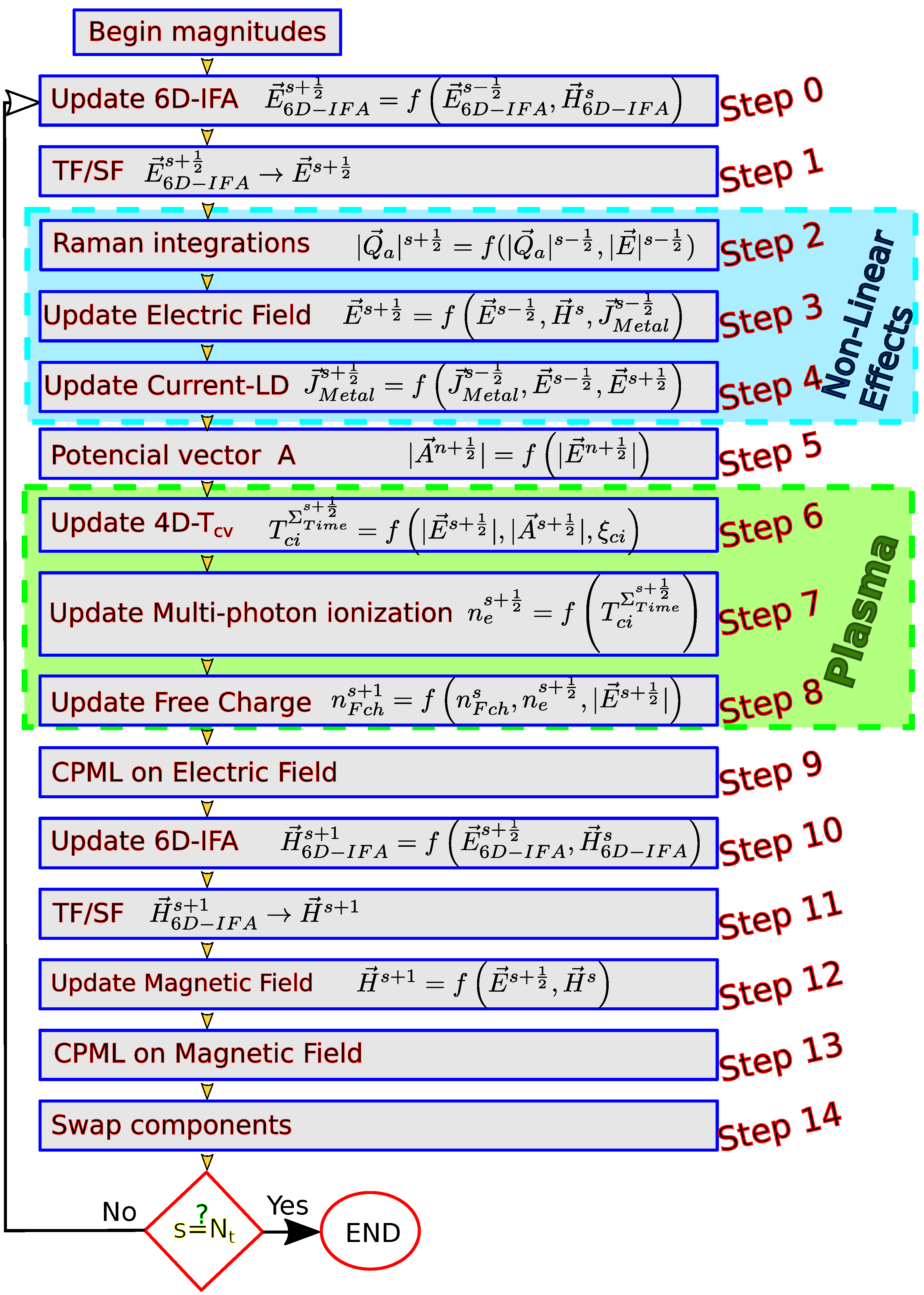
	$n_{f{e}^{-}}^s=n_{f{e}^{-}}^{s+1}$; ${\overrightarrow{H}}^s={\overrightarrow{H}}^{s+1}$; $|{\overrightarrow{Q}}_a^{s-\frac{1}{2}}|=|{\overrightarrow{Q}}_a^{s+\frac{1}{2}}|$;

summarizes the algorithms presented in this section, and Figure 2 sketches the general flow chart. In the next section, we discuss the stability conditions for these algorithms.

In Appendix A, we determine the stability conditions for the presented algorithms.

Table 2. List of stability conditions. Note that $Min\left[\right]$ selects the minimum value in a list.

Stability Conditions
All cases	${\Delta }_t\le \frac{n_i}{c_0}\sqrt{\frac{1}{{\Delta }_x^2}+\frac{1}{{\Delta }_y^2}+\frac{1}{{\Delta }_z^2}}$
Metal	$\mathcal{R}\left[a\right]\ge 0$	$\mathcal{R}\left[b\right]\ge 0$
Kerr	$|{\tilde{\overrightarrow{E}}}_0|<\sqrt{\frac{{ϵ}_{\infty }}{D_f{\chi }_0^{\left(3\right)}}}Min\left[\frac{1}{\sqrt{\alpha }},\frac{1}{\sqrt{1-\alpha }}\right]$
Raman
Photoionization	${\sigma }_{f{e}^{-}}\ge 0$

summarizes the stability conditions of all these effects together or separately.

4. Performance and Framework

Some approximations made here are not always applicable and, in this section, we will establish the validity framework of the proposed algorithms. In particular, we should consider the two approximations ${\int }_0^{\left(s+\frac{1}{2}\right){\Delta }_t}\delta (t-\tau )|\overrightarrow{E}(\overrightarrow{r},\tau )|d\tau \simeq {\int }_0^{\left(s-\frac{1}{2}\right){\Delta }_t}\delta (t-\tau )|\overrightarrow{E}(\overrightarrow{r},\tau )|d\tau$ and $|{\overrightarrow{Q}}_a^{s+\frac{1}{2}}|=|{\overrightarrow{Q}}_a^{s-\frac{1}{2}}|+\overline{\overline{g}}\left((s-n{t}_0\left(k\right)){\Delta }_t\right){|{\overrightarrow{E}}^{s-\frac{1}{2}}|}^2$. Both expression are derived in [9] under the Born–Oppenheimer approximation [4] where the Kerr non-resonant virtual electronic transitions are in the order of 1fs, so it can be considered an instantaneous event, which is modeled by the Dirac delta function. However, while the time stepping keeps beneath 1 fs, we could model the medium reaction by using a time narrow Gaussian function with a standard deviation of 1 fs. In our simulations, ${\Delta }_t\sim 0.1$ fs, so we are adding in a fraction of $\frac{1}{10}$ the standard deviation. In this particular situation, the approximation is assumed to be valid. We employ the full explicit form $|{\overrightarrow{Q}}_a^{s+\frac{1}{2}}|=|{\overrightarrow{Q}}_a^{s-\frac{1}{2}}|+\overline{\overline{g}}\left((s-nt\left(k\right)){\Delta }_t\right){|{\overrightarrow{E}}^{s-\frac{1}{2}}|}^2$ in the place of right implicit form $|{\overrightarrow{Q}}_a^{s+\frac{1}{2}}|=|{\overrightarrow{Q}}_a^{s-\frac{1}{2}}|+\overline{\overline{g}}\left((s-nt\left(k\right)){\Delta }_t\right){\left|\frac{{\overrightarrow{E}}^{s+\frac{1}{2}}+{\overrightarrow{E}}^{s-\frac{1}{2}}}{2}\right|}^2$ based on the same idea than before, ${\Delta }_t\ll {\tau }_1$ and ${\Delta }_t\ll {\tau }_2$ so $e^{\frac{-(t+{\Delta }_t)}{{\tau }_1}sin\left(\frac{t+{\Delta }_t}{{\tau }_2}\right)}\backsimeq e^{\frac{-\left(t\right)}{{\tau }_1}sin\left(\frac{t}{{\tau }_2}\right)}$. This expression is valid for all instant $\forall t$. 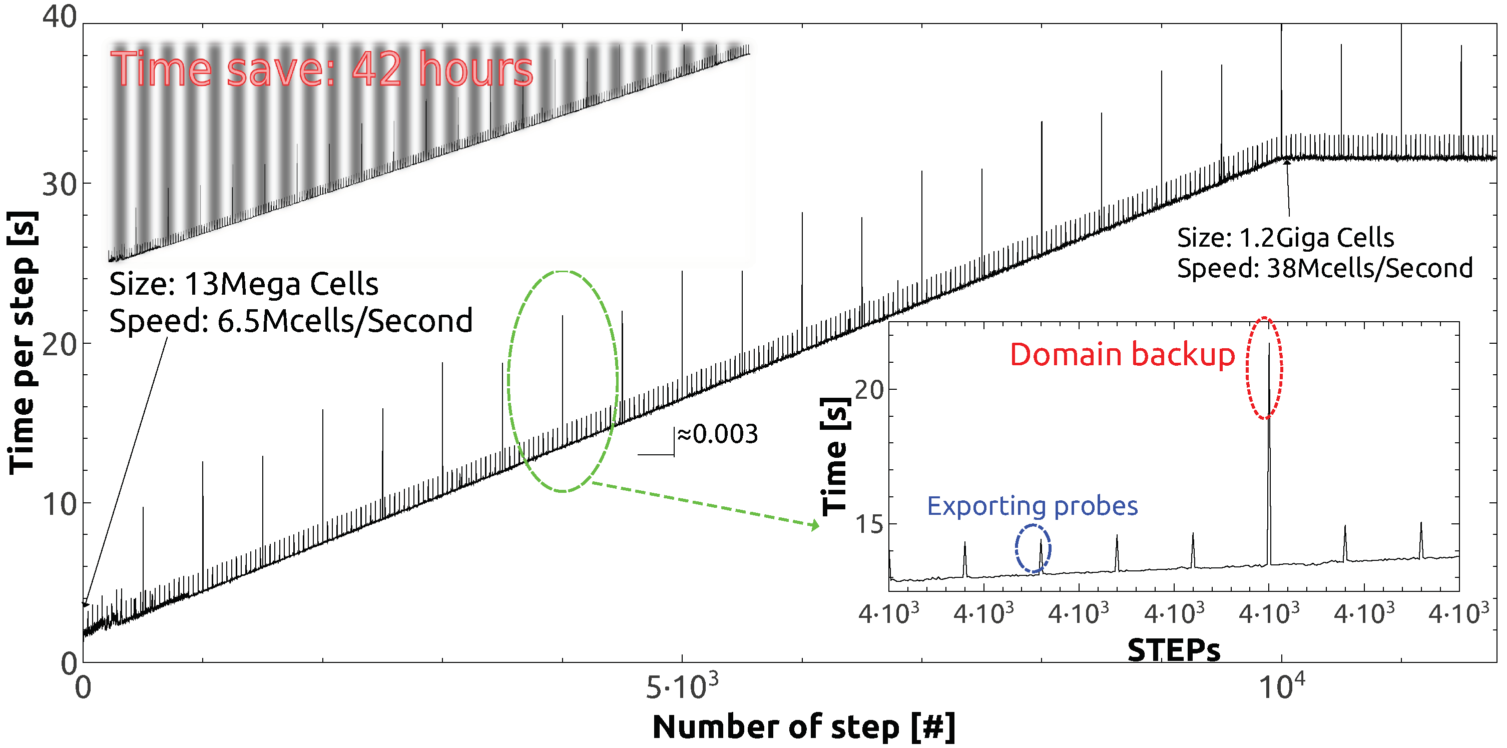Hence, we fix the limit for this full explicit approach in the relation ${\Delta }_t<1$ fs. The advantage of a fully explicit approach concerns the simulation time. Due to the updating connection in an implicit scheme, most of the algorithms should be re-updating to advance a time step. In classical FDTD, it is usually fixing the limits of the index in all nested loops. In a significant computational domain, for instance, 1.2 G cells, the updating demands 30 s. If the algorithm has to be repeated at least three times, the simulation should need around three times the the implicit scheme. Figure 3 shows the number of simulation status updates on the abscissa axis and on the ordinate axis the time needed in order to update these simulation states. Each step or update corresponds to executing the 14 algorithms shown by Figure 2. In addition to these algorithms that are necessary to perform a system status update, two numerical processes are employed. One exports simulation data or results (every 40 updates) and the other exports the complete simulation status (every 500 updates). The latter is done for two reasons. The first is to recover a state of a simulation in case of computer collapse (for example a failure in the computer electric power source). The second reason concerns the alteration of the computational domain (electromagnetic properties or/and size of the computational domain) without the need to restart the simulation from the first time stepping. In Appendix B the

Table A1. Computational resources.

Computational Resources:
CPU: Intel Core i9-10980XE
MB: GIGABYTE X299X
RAM: Crucial CT32G4RF D4293 DDR4-2933
ROM: 2x Crucial P5 1TB PCIe M.2 2280SS SSD
GPU: GeForce GTX 1080 Ti

lists the computational resources employed in the simulations. Under these conditions we reach a performance which can be summarized by the computational burdens and some performance parameters. Those relies on a computational domain size of 121.5 GBs in RAM, a maximum number of Yee’s cell charged and computed of 1.2 Giga cells, a minimum number of Yee’s cell computed of 13 Mega cells, a speed at minimum and maximum load of 6.5 Mcells/s and 38 Mcells/s respectability, a probe exportation time of 1.47 s and a computational domain backup time of 8.76 s. Therefore, Figure 3 depicts the time performance for a simulation carried out with dynamics nested loops. In our scheme, the size of the nested loops is provided by the information created. We know that our implementation violates the second rule of NASA’s Ten-Rules for Developing Safety Critical Code [19]. In general, it is a good practice to arrange the loop indexes in the simulation beginning and keep these ranges. By doing this, we fix, from the start, the nested loop size. Nevertheless, the employment of a dynamic nested loop saves simulation time. Figure 3 depicts that we save more than forty hours. In a simulation with the same characteristics and static nested loop, we should have a constant duration per time step updating of 32 seconds which is equal to the asymptotic value in Figure 3. The total simulation duration is the accumulated time or area under the plot schematized in Figure 3. Hence, the triangle in gray color is the time saved by means of dynamic nested loops.

Finally, we close this section with some consideration on Equation (3). This equation is a derivation from the charge/electrons continuity equation [20], which has the general form $\frac{\partial \rho \left(\overrightarrow{r},t\right)}{\partial t}=q\left(G\left(\overrightarrow{r},t\right)-R\left(\overrightarrow{r},t\right)\right)-\nabla ·\overrightarrow{J}\left(\overrightarrow{r},t\right)$, where we neglect the term $\nabla ·\overrightarrow{J}\left(\overrightarrow{r},t\right)\ll q{n}_{f{e}^{-}}\left(\overrightarrow{r},t\right)$. We know from theory that $\rho \left(\overrightarrow{r},t\right)=q{n}_{f{e}^{-}}\left(\overrightarrow{r},t\right)$ and $\overrightarrow{J}\left(\overrightarrow{r},t\right)=q{\mu }_{f{e}^{-}}{n}_{f{e}^{-}}\left(\overrightarrow{r},t\right)\overrightarrow{E}\left(\overrightarrow{r},t\right)$. The key is the extremely low mobility ${\mu }_{f{e}^{-}}\sim {10}^{-22}$, which is deduced from [21]. We can consider a highly intense laser beam with $|\overrightarrow{E}\left(\overrightarrow{r},t\right){|}^2\sim {10}^{13}$, which induces a free electron concentration in fused silica of $n_{f{e}^{-}}\left(\overrightarrow{r},t\right)\sim {10}^{26}$ and compare with $\frac{\nabla ·\overrightarrow{J}\left(\overrightarrow{r},t\right)}{q}\sim \frac{\frac{{10}^{-22}\times q{10}^{26}\times {10}^{13/2}}{{10}^{-7}}}{q}\sim {10}^{18}$. Therefore, we can conclude that $n_{f{e}^{-}}\left(\overrightarrow{r},t\right)\sim {10}^8\frac{\nabla ·\overrightarrow{J}\left(\overrightarrow{r},t\right)}{q}$ and Equation (3) is a valid approximation in the present context.

5. Results

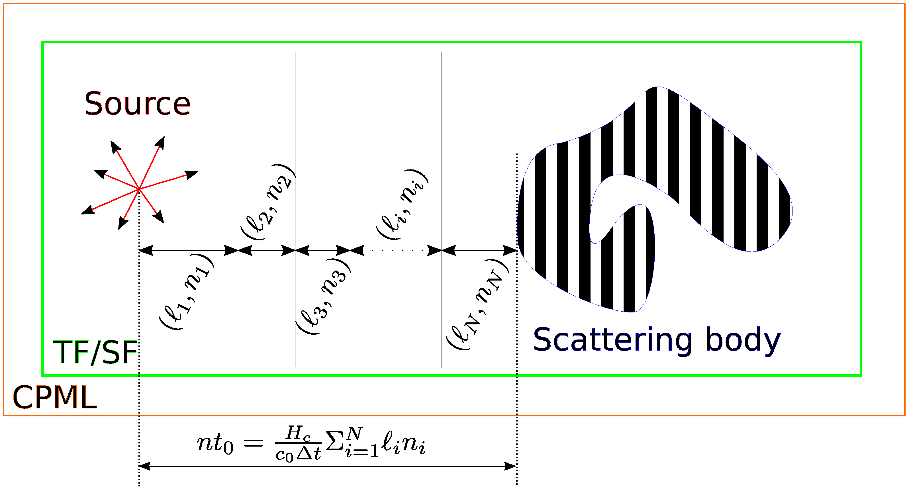
An efficient technique to compute scattered fields in the context of FDTD modeling is the total-field/scattered-field (TF/SF) incident wave source, which is employed by most all current commercial FDTD solvers [2]. Fundamentally, the TF/SF technique is an application of the well-known electromagnetic field equivalence principle [22]. By this principle, the original incident wave of infinite extent and arbitrary propagation direction, polarization, and time-waveform is replaced by electric and magnetic current sources appropriately defined on a finite closed surface, called the Huygens surface [23], containing the object of interest. The reformulated problem confines the incident illumination to a compact total-field region and provides a finite scattered-field region external to the total-field region that is terminated by an absorbing boundary condition (ABC) to simulate the FDTD grid extending to infinity. In particular, we use convolutional perfectly matched layers, a technique already used in other works [24]. In this work, we have used the finite-difference time-domain discrete plane wave technique (FDTD-DPW), which is a numerical approach based on TF/SF technique that allows one to propagate plane waves quasi-perfectly isolated [25]. This means a propagation in the total field domain without reflections to the scattered field domain on the order of machine precision (∼300 dB) [26]. This technique is valid for any angle of propagation, for any grid cell aspect ratio and even for nonuniform grids [27]. 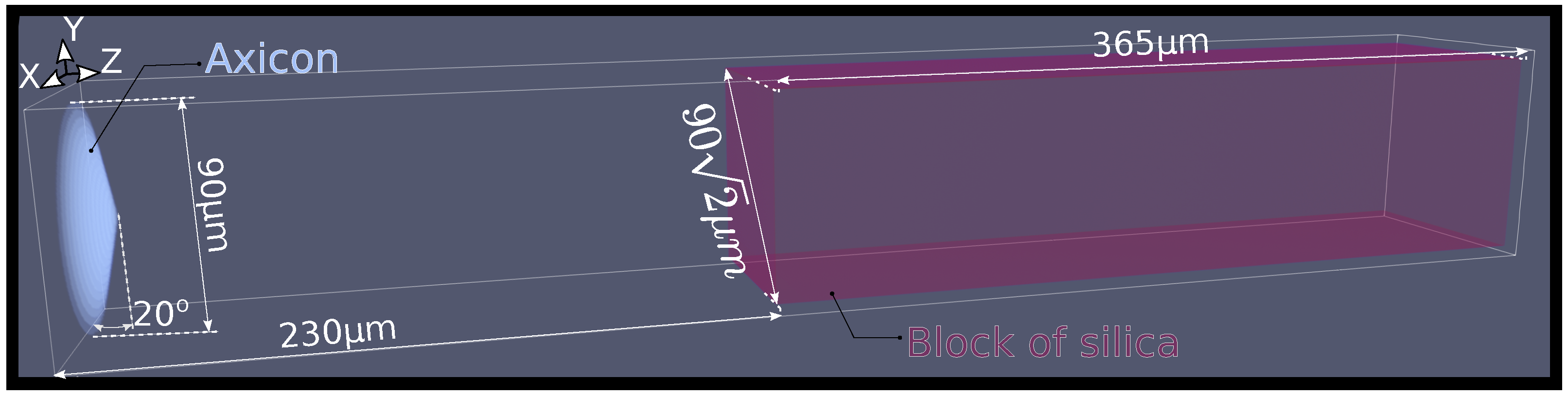Figure 4 illustrates the total field region where there are two important elements, an axicon lens that generates the Bessel beam from the initial plane waves and a block of fused silica. In this domain, the incident plane wave is generated by the FDTD-DPW scheme.

The calculation domain contains a block of fused silica glass where the nonlinear effects apply. The interaction between the incident plane wave and the axicon lens results in a Bessel beam, which impinges the SiO${}_2$ block. We assume a pulsed laser source of wavelength $(800\pm 11)$ nm and a time full width at half maximum of ${\sigma }_t=$ 40 fs. The pulsed incident time-waveform is modeled by $h\left(t\right)=A\left(t\right){\mathrm{sech}}^2\left(\frac{t-{\mathrm{t}}_0}{{\sigma }_t}\right)sin\left(t\omega \right)$, where $A\left(t\right)={\left(\frac{tanh\left(t\omega \right)+1}{2}\right)}^{\varsigma }$ with $\varsigma \ge 1$, is an appropriate way to avoid numerical instabilities in the simulation beginning. The incident field six-dimensional array (IFA) that feeds the FDTD-DPW is quite simple $\overrightarrow{E}\left({\overrightarrow{r}}_{IFA,t}\right)=E_{0}h\left(t\right)\widehat{x}$. In addition, there are other parameters that characterized the media properties and are summarize in

Table 3. Media main parameters.

Parameters
Name	Symbol	Value	Unit	Ref.
Gap energy	$E_g$	9	eV	[28]
Third-order elec-tric susceptibility	${\chi }_0^{\left(3\right)}$	${10}^{-22}$	$\frac{{\mathrm{m}}^2}{{\mathrm{V}}^2}$	[28]
Raman sinusoidal time	${\tau }_1$	12.2	fs	[29]
Raman response fraction	$1-\alpha$	0.18	-	[29]
Electron recombi-nation time	${\tau }_r$	150	fs	[10]
Mobility	${\mu }_{f{e}^{-}}$	$1.13\times {10}^{-22}$	$\frac{{\mathrm{m}}^2}{\mathrm{Vs}}$	[21]
Density of valence electrons	$N_0$	${10}^{22}$	${\mathrm{cm}}^{-3}$	[10]
Electron mass reduced particle	$m_{vc}^{*}$	0.5	${\mathrm{m}}_0$	[10]
Work function	$W_f$	5	eV	[28]
Avalanche ioniza-tion coefficient	$\Theta$	10${}^{-3}$	$\frac{{\mathrm{m}}^2}{\mathrm{Ws}}$	[28]
Raman decay time	${\tau }_2$	32	fs	[29]
Kerr response fraction	$\alpha$	0.82	-	[29]
Laser characteristic time for electrons production	${\tau }_d$	3	ps	[10]
Impact ionization efficiency	$\eta$	0.01	-	[28]
Fitting parameter for the spatial expansion of the valence wave function	$\mathsf{\Omega }$	0.8	-	[10]
Metal	a	$19.2+j2.7$	PHz
parameters	b	$1.3-j3.9$	PHz	[15]
Axicon refractive index	$n_a$	1.45	-	[30]

.

By using the developed irradiation strategy, the computational domain elements and their properties as well as the algorithm we carried out, the obtained results can be divided into three groups:

• Low power regime: $E_0={10}^4\frac{\mathrm{V}}{\mathrm{m}}$ and $I=2.46\times {10}^{14}\frac{\mathrm{W}}{{\mathrm{m}}^2}$.
• Critical power regime: $E_0=3.5\times {10}^5\frac{\mathrm{V}}{\mathrm{m}}$ and $I=8.61\times {10}^{16}\frac{\mathrm{W}}{{\mathrm{m}}^2}$.
• High power regime: $E_0={10}^6\frac{\mathrm{V}}{\mathrm{m}}$ and $I=2.45\times {10}^{18}\frac{\mathrm{W}}{{\mathrm{m}}^2}$.

The power intensity $I=Max\left(\tilde{I}\left(\overrightarrow{r},t\right)\right)$ is calculated as the maximum power that flows through a section of ${\sigma }_w^2$, being ${\sigma }_w$ the pulsed laser transverse waist, ${\sigma }_{\ell }$ the pulsed length in the propagation direction and $z_p$ the central pulse location at the calculation time. Hence, $\tilde{I}\left(\overrightarrow{r},t\right)=\underset{-{\sigma }_w}{\overset{{\sigma }_w}{\int \int }}dxdy\underset{z_p-{\sigma }_{\ell }}{\overset{z_p+{\sigma }_{\ell }}{\int }}dz\widehat{z}·\frac{\overrightarrow{S}\left(\overrightarrow{r},t\right)}{{\sigma }_w^2}$.

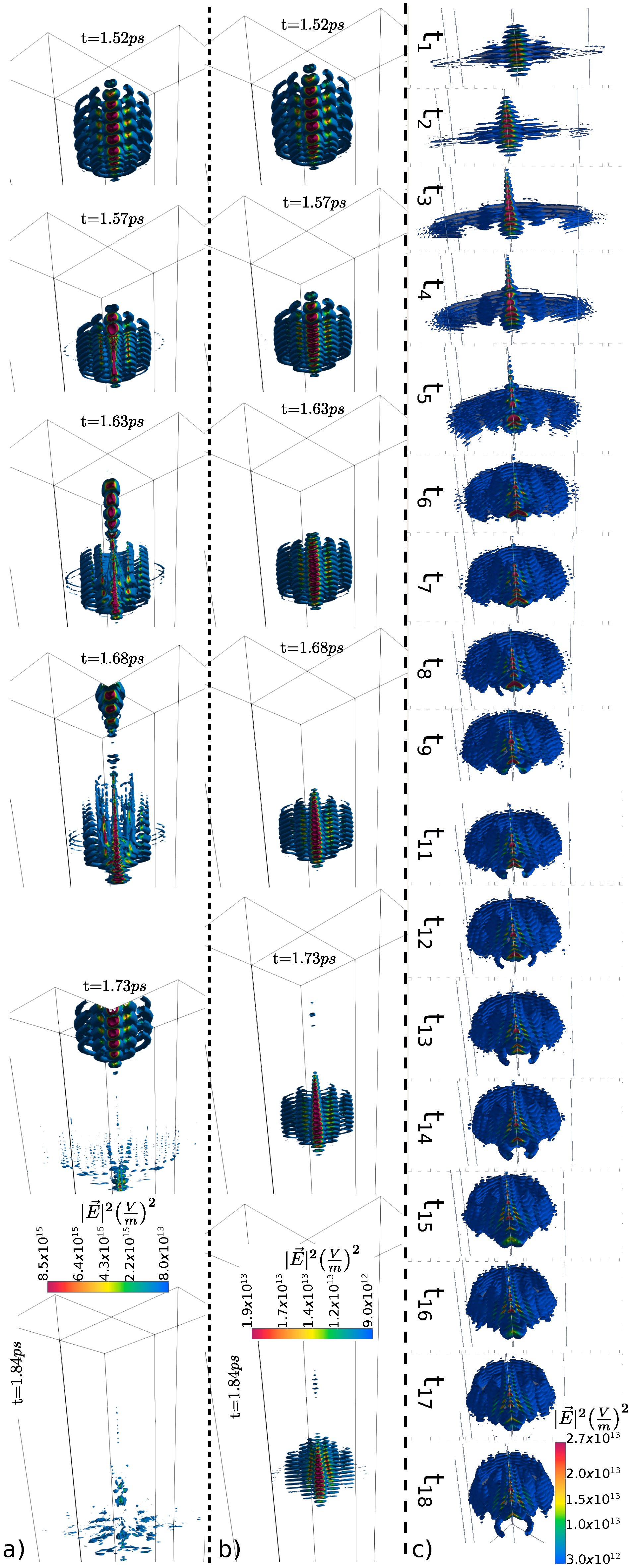
To validate the algorithm, which includes nonlinear effects during light propagation, we have investigated the features of the propagation regime depending on the laser intensity. Figure 5a,b redraw the distribution evolution of the pulsed square electric field module for simulation performed for different laser intensity sources. Figure 5a plots the iso-slices that depicts $|\overrightarrow{E}{|}^2$ inside the fused silica bulk for high laser power in the system. From top to bottom, the time evolution sequence reveals the defocusing process of the Bessel beam, which ends by forming some filamentation structures in the light distribution. At the time $t=5720,{\Delta }_t=1.52$ ps, the pulsed square electric field module begins to penetrate the interface air-fused silica. All successive time plots correspond to a propagation inside the fused silica block. Figure 5b illustrates, for the same time moments, but a higher initial power source, the square electric field module during the propagation inside SiO${}_2$ material.

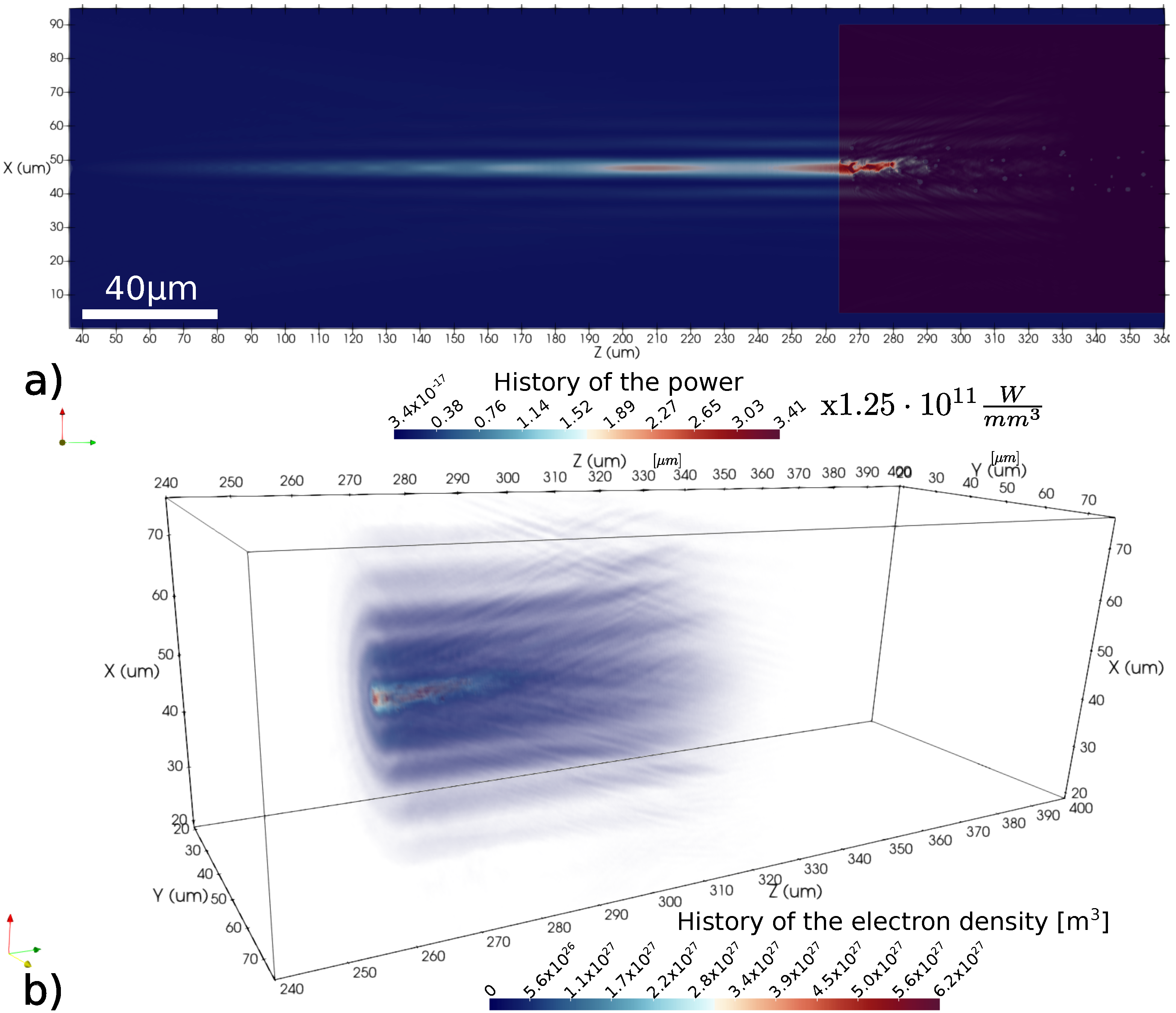
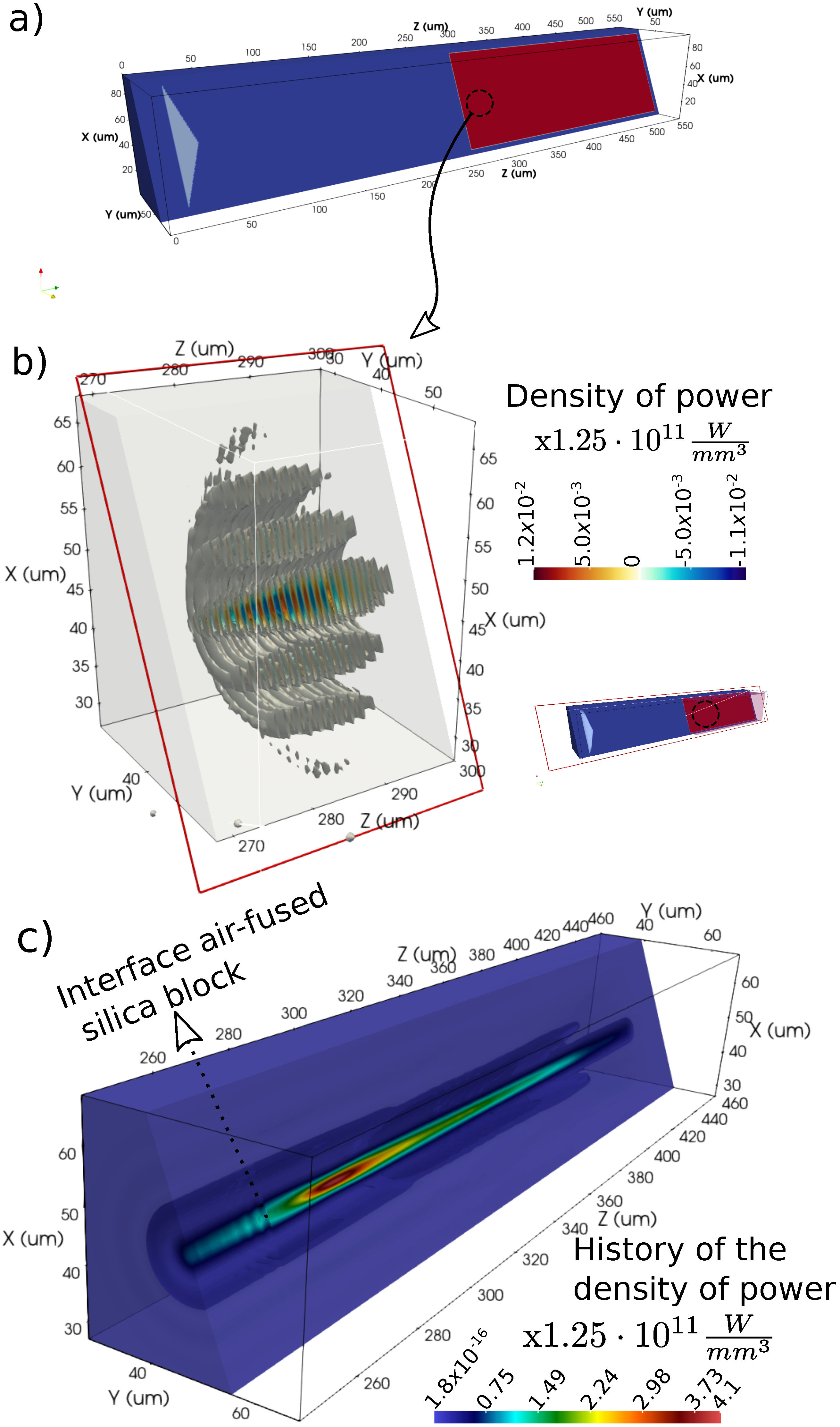
We complement the picture with a simulation carried out in the medium power regime. From the instant of time, $t_1=1.67$ ps to the instant $t_{18}=2.56$ ps, Figure 5c illustrates the antagonistic trade-off between the focusing and the defocusing process experienced by the Bessel beam along with its travel through the bulk fused silica target. Figure 6b shows the history of the power density at the critical threshold separating medium and high power regimes, along with a few steps of time. In this figure we can identify the interface air-fused silica due to the rings which record the history of a stationary wave formed after the interaction. We can observe a strong focusing process in the entrance of the fused silica block followed by an alternation of refocusing and the defocusing events induced and governed by the photoionization and Kerr effect competition, and we know that these are not diffraction artifacts because in the air, at the same laser intensity, we do not observe them. At this stage, we have to give a clear definition of the pulsed power density and the power history. The magnitude of pulsed power density is defined as $\nabla ·\overrightarrow{S}\left(\overrightarrow{r},t\right)$, where $\overrightarrow{S}\left(\overrightarrow{r},t\right)=\overrightarrow{E}\left(\overrightarrow{r},t\right)\wedge \overrightarrow{H}\left(\overrightarrow{r},t\right)$ is the Poynting vector [31]. Figure 6a sketches the pulsed power density. From this magnitude $\nabla ·\overrightarrow{S}\left(\overrightarrow{r},t\right)$, we can calculate the delivered pulsed electromagnetic density of energy ${\int }_0^{t^{\prime }}\nabla ·\overrightarrow{S}\left(\overrightarrow{r},t\right)dt$. Besides this, it is interesting to consider the range of values in Figure 6a. We can identify a negative power density that requires clarification. As the Poynting vector represents the flux of power through a given surface, the divergence of this magnitude represents the power density that comes into/out a particular point in a given region. In particular, in FDTD calculations, we are describing the power flux through the computational nodes that discretized the computational domain. In the density power accounting, the reference system is placed inside the cell that encloses the nodes. In this way, a negative power density, in a particular instance of time, in a local region, means a local sink of power $\nabla ·\overrightarrow{S}\left(\overrightarrow{r},t\right)<0$ in that region, and vice versa, we have a local source of power as $\nabla ·\overrightarrow{S}\left(\overrightarrow{r},t\right)>0$. These oscillations in the density power magnitude indicate a redistribution that is able to support the pulsed density power and the pulsed density energy traveling.

Turning to the matter at hand, we define the history of the power density by applying the absolute value to the divergence of the Poynting vector $|\nabla ·\overrightarrow{S}\left(\overrightarrow{r},t\right)|$.

The bi-dimensional longitudinal cut of the history of the power density depicted in Figure 6b permits one to identify the air–fused silica interface. There, in that interface, we can appreciate the reflected beam and the strong focusing in the entrance due to the Kerr effect. We assume the same refractive index for both the axicon lens and the fused silica block in which the wave Bessel beam impinges.

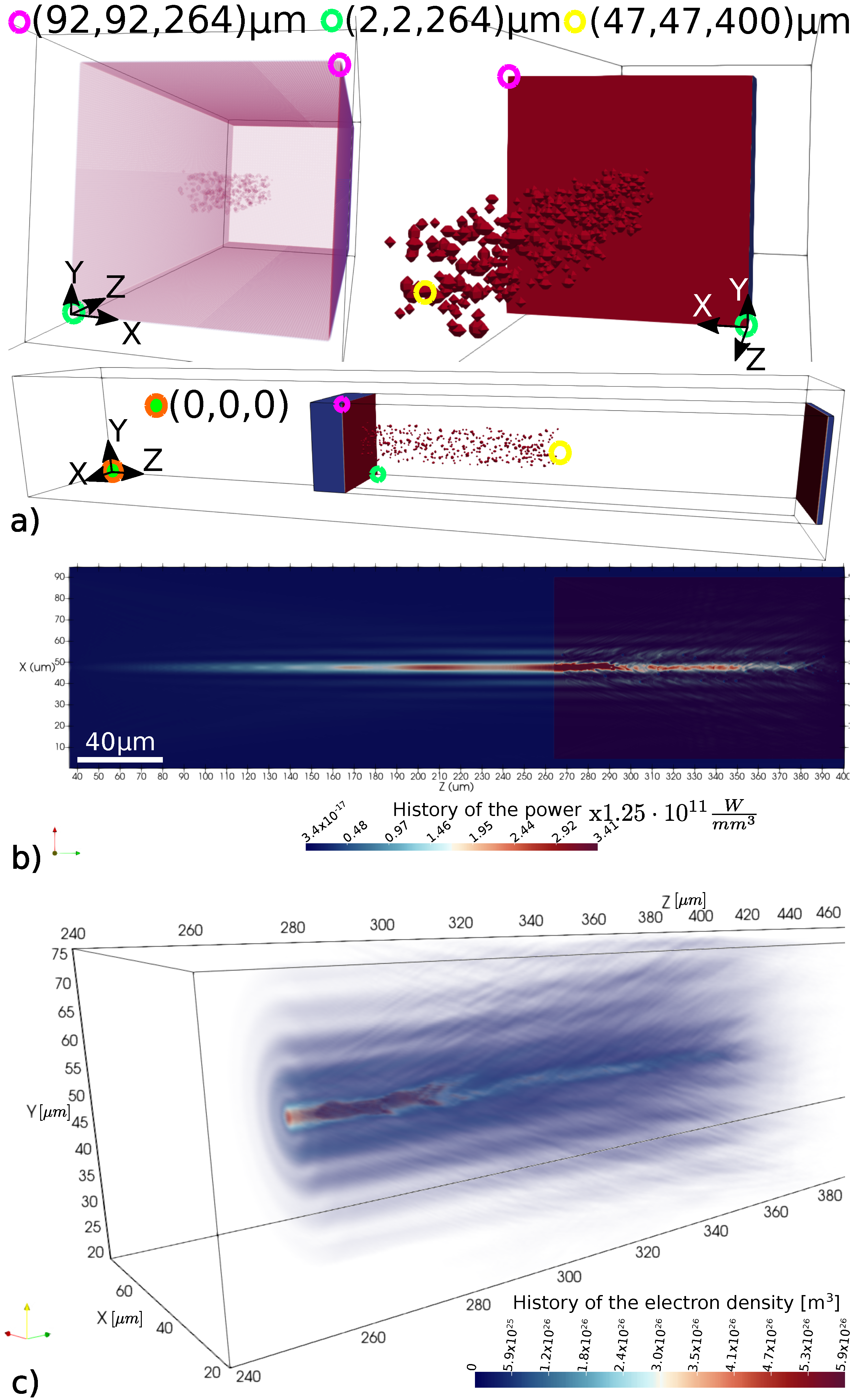
Although we assume nonlinear media, in the simulation results presented up to this point in the manuscript, we have considered that the fused silica is isotropic and homogeneous. However, in order to study the effect of micro- and nanopores in the fused silica, 650 regions or voids have been introduced that range in size from 200 to 650 nanometers in radius. These spherical embedded cavities, that are plotted in Figure 7a, emulate a nanoporous fused silica bulk. The traditional method of linear combined congruence random number generators has been used to assign the size and location of these pores of air/void particles. The linear congruential generator yields a sequence of pseudo-randomized numbers calculated with a discontinuous piecewise linear equation. The most important thing about the method is that, under the same seeds, the same random number distributions will be obtained, which allows us to reproduce both size distributions and particle locations. This will be useful to evaluate the effects resulting from another kind of media, such as metal particles, which will allow us to make a point-to-point comparison and infer conclusions from the results. In this setup, Figure 7b shows the history of the power in the region where the particles are located. The simulation is stopped when the nonlinear Bessel beam exits the porous fused silica region. Looking at Figure 7c, it appears that a correlation can be made between the distribution of photoionized electrons and the laser power density, in full consistency with our model. Figure 7c shows a history of the density of the ionized electrons as a consequence of the Bessel beam, which travels through the fused silica block. This result leads us to conjecture that both quantities look similar in terms of spatial structure.

It is relevant to study the distribution or history of power in a non-homogeneous dielectric, as is the present case. If we observe Figure 7b in detail, we see that the history of power reveals the history of field intensity as it passes through the nanoporous medium of SiO${}_2$. Due to a simple matter of impedance, the wavefront of the pulse is redistributed, avoiding entering inside the voids. As we can see in the longitudinal section shown by Figure 7b, the power vanishes inside the voids and the maximum power is not found at the interface fused silica-void. The maximum is reached in the glass medium between the pores. There is a visual explanation for this behavior. In some lenses, an anti-coating multi-layer that matches the impedance of the lens with the surrounding media (in general, glasses could be done for water or air), is coupled in order to remove the reflections. This gradient in the refractive index is necessary to facilitate the flowing energy from the lens to the environment. In the porous fused silica, there is an abrupt change in the refractive index that explains our result.

There is a Supplementary Material consisting in a video animation (see the link https://youtu.be/nvGdtxQ9E8o) that shows dynamically the ultrafast pulsed Bessel beam, depicted by employing the pulsed electric field module, that crosses the interface air-fused silica and travels through a fused silica block with air nanovoids.

As stated above, we have followed identical reasoning and repeat the simulation, this time replacing nanovoids with metal particles. The results are shown in Figure 8. Figure 8a illustrates the power history under the same intensity of light. Along the photoexcitation path, the maximum power occurs around the metal– fused silica interface, enhancing and localizing the light coupling to the nanocomposite material. Even if the non-diffractive behavior is still present, it is less observable, as the beam is strongly attenuated by metal absorption. Moreover, the arrangement of the higher region of light absorption follows the randomly distributed composition of the metallic sphere. This indicates that contrary to dielectric–void interfaces, the dielectric-metal region fosters local effects, preventing any collective response of the medium. This statement may differ if the particles are judiciously defined in terms of concentration and size in order to enhance resonance effects as plasmonic modes. 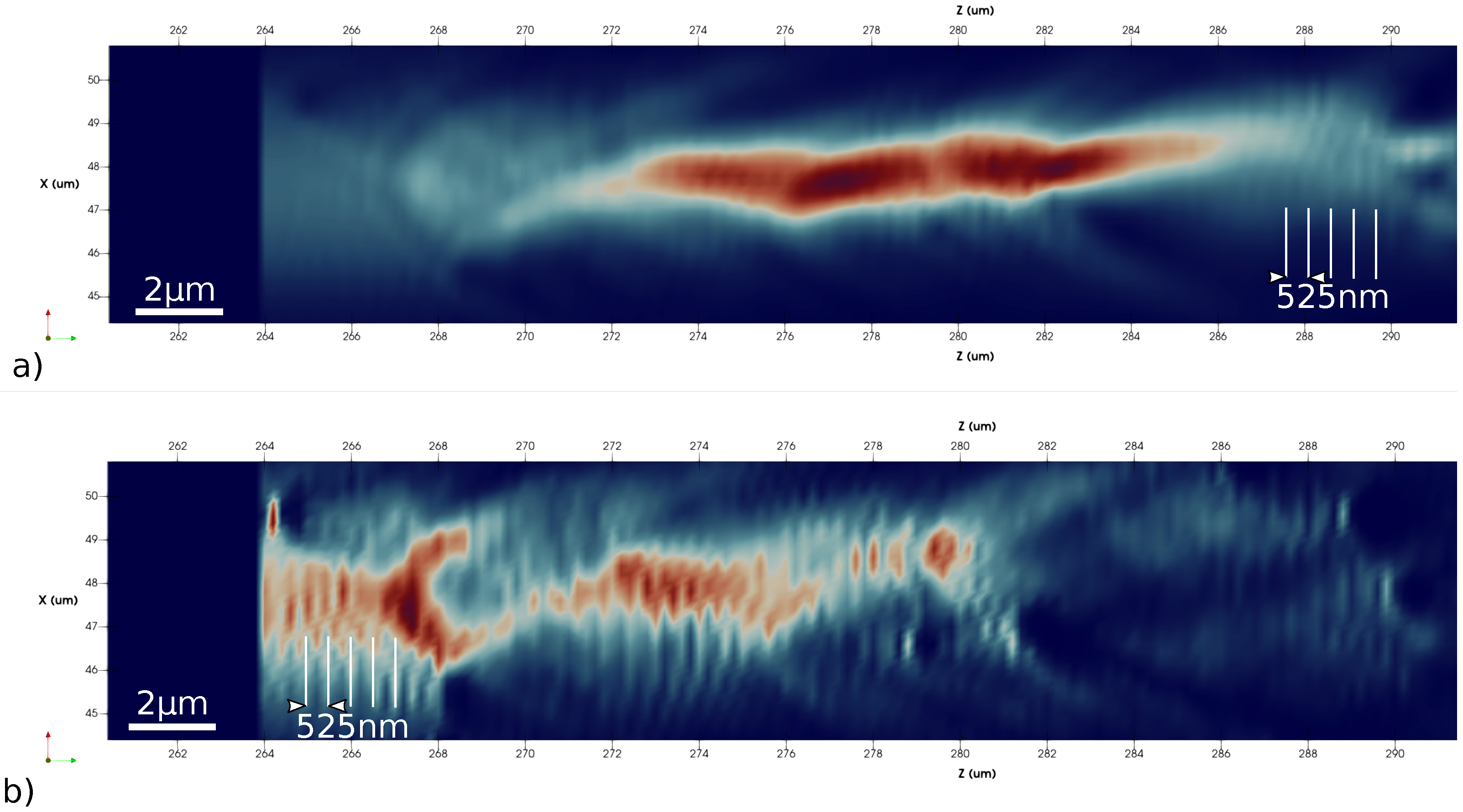In Figure 9, we observe a pattern in the electron photoionized history. In particular, Figure 9a depicts a weak structure of parallel planes, which is more intense in some regions. Figure 9b shows a stronger pattern. The present results, sketched by Figure 9a, reveal that ultrashort laser pulse interacting with distributed performed scattering nanovoids induces local field enhancement that results in enhanced nonlinear absorption and localized optical breakdown. At the void-SiO${}_2$ interface, the multiphotonic ionization process transforms the material into a thin layer of absorbing plasma with metallic-like properties. The light coupling initiates the growth of nanoplates of enhanced energy deposition, perpendicular to laser propagation direction, but parallel to the polarization. This kind of arranged structure exhibiting a periodicity approximately the wavelength of light in fused silica was commonly experimentally reported in conditions of tightly focused and high repetition rate [32,33]. They directly emerge from the spatial coherence of the waves scattered from the inhomogeneous material in the plane perpendicular to the beam propagation direction. Note the relatively used large nanovoids associated to the grid resolution do not allow to discriminate nanogratings of higher frequency perpendicular to the electric field. For propagation inside laser-induced nanoporous media, the fused silica glass remains underdense, below the critical plasma concentration, and the standing wave effect remains weak. However, the other simulation conditions, portrayed in Figure 9b), clearly indicate that for metallic nanoparticles, local field enhancement occurs near the metal-dielectric interface [34]. Upon electron–matrix energy coupling and void deformation, the light pattern may result in elongated nanostructures [35]. This shows that nanoplasmonic behavior dominates and opens the route for advanced applications as embedded micro-reflectors for a stronger near-field interaction regime.

Propagation and scattering through sphere inclusions with different optical properties demonstrate that the current algorithms are stable and can model efficiently nonlinear media with sharp dielectric interfaces among them. Moreover, nonlinear metal–dielectric interface investigations are far reaching for technology-based photonics. For instance, in a wider frequency spectrum, resonators, metasurfaces with designed cavities, metal–dielectric waveguides or even coating optical fibers are composed of metal–dielectric interfaces that may involve simultaneously nonlinear mechanisms of different nature. If we imagine for a sake of simplicity an harmonic electromagnetic pulse, which is guided, for instance, inside of a optical fiber, we should solve two coupled inhomogeneous Helmholtz’s equations in the frequency domain ${\nabla }^2\overrightarrow{\tilde{E}}\left(\overrightarrow{r}\right)+{\omega }^2\mu ϵ\left(\overrightarrow{r}\right)\overrightarrow{\tilde{E}}\left(\overrightarrow{r}\right)=-\nabla \left(\overrightarrow{\tilde{E}}\left(\overrightarrow{r}\right)·\nabla \left(ln\left(ϵ\left(\overrightarrow{r}\right)\right)\right)\right)$ and ${\nabla }^2\overrightarrow{\tilde{H}}\left(\overrightarrow{r}\right)+{\omega }^2\mu ϵ\left(\overrightarrow{r}\right)\overrightarrow{\tilde{H}}\left(\overrightarrow{r}\right)\left(\overrightarrow{r}\right)=(\nabla \wedge \overrightarrow{\tilde{H}}\left(\overrightarrow{r}\right))\wedge \nabla ln\left(ϵ\left(\overrightarrow{r}\right)\right)$. In these equations, the refractive index $n\left(\overrightarrow{r}\right)=\sqrt{{ϵ}_r\left(\overrightarrow{r}\right){\mu }_r}$, which is a dynamic magnitude along the pulsed beam propagation or simply a nonlinear magnitude, has to be taken into consideration. In this way, the algorithms present here can be used to deal with this kind of problems.

6. Conclusions

In this work, we have proposed a numerical approach for nonlinear laser beam propagation based on the time-domain discretization of Maxwell equations in a fully explicit scheme, including four nonlinear optical effects. The developed algorithms have been benchmarked in three different ways. First, we have studied the algorithm’s stability conditions by combining the von Neumann method with the Routh–Hurwitz criterion. Second, we have established the physical framework for the algorithms, with special attention given to the approximation carried out in the algorithm derivation. Third, we have employed the algorithms in order to determine the transient optical properties of a photoexcited media when a laser beam is focused inside a fused silica bulk. In particular, we have considered a Bessel beam as a free-diffraction beam due to its stable and rebuildable-like energy distribution along with electromagnetic pulse travel path. This non-diffractive behavior has been observed numerically by tracking the power/energy history. This has been determined by evaluating the absolute value of the power $|\nabla ·\overrightarrow{S}\left(\overrightarrow{r},t\right)|$ and the density energy history as ${\int }_0^{t^{\prime }}|\nabla ·\overrightarrow{S}\left(\overrightarrow{r},t\right)|dt$. The main advantage of the present method consists of its remarkable numerical performance (see Figure 3), that together with the tolerant stability conditions found out and the accuracy results, under an also permissive physical framework, made it valid for a wide range of applications (such as ultrafast laser processing which has been extensively applied to fabricate 3D photonic devices based on embedded optical waveguides inscribed in glass materials by inducing permanent refractive index changes in the focal volumes [36], optical couplers and splitters [37], volume Bragg gratings [38], or even diffractive lenses [39] which have been efficiently inscribed by refractive-index changes during light propagation) in which optical/electromagnetic nonlinear effects have to be taken into consideration. Finally, our approach is generalizable to any nonlinear electromagnetic problem with dielectric–metal interfaces. The proposed work elucidates the simultaneous treatment of nonlinear effects and provides new routes toward the simulation of light–matter interaction with sub-wavelength features for the optimization of guided structures or loss-free metasurfaces.

References

1. Greene, J.H.; Taflove, A. General vector auxiliary differential equation finite-difference time-domain method for nonlinear optics. Opt. Express 2006, 14, 8305–8310. [Google Scholar] [CrossRef] [Green Version]
2. Taflove, A.; Oskooi, A.; Johnson, S. Advances in FDTD Computational Electrodynamics: Photonics and Nanotechnology; Artech House Antennas and Propagation Library; Artech House: Norwood, MA, USA, 2013. [Google Scholar]
3. Maksymov, I.S.; Sukhorukov, A.A.; Lavrinenko, A.V.; Kivshar, Y.S. Comparative Study of FDTD-Adopted Numerical Algorithms for Kerr Nonlinearities. IEEE Antennas Wirel. Propag. Lett. 2011, 10, 143–146. [Google Scholar] [CrossRef]
4. Hellwarth, R. Third-order optical susceptibilities of liquids and solids. Prog. Quantum Electron. 1977, 5, 1–68. [Google Scholar] [CrossRef]
5. Jia, H.; Li, J.; Fang, Z.; Li, M. A new FDTD scheme for Maxwell’s equations in Kerr-type nonlinear media. Numer. Algorithms 2019, 82, 223–243. [Google Scholar] [CrossRef]
6. Weber, W.H.; Ford, G.W. Optical electric-field enhancement at a metal surface arising from surface-plasmon excitation. Opt. Lett. 1981, 6, 122–124. [Google Scholar] [CrossRef]
7. Yu, H.; Peng, Y.; Yang, Y.; Li, Z.Y. Plasmon-enhanced light–matter interactions and applications. NPJ Comput. Mater. 2019, 5, 1–14. [Google Scholar] [CrossRef]
8. Moreno, E.; Sohrabi, R.; Klochok, G.; Michael, E. Vertical versus planar pulsed photoconductive antennas that emit in the terahertz regime. Optik 2018, 166, 257–269. [Google Scholar] [CrossRef]
9. Blow, K.J.; Wood, D. Theoretical description of transient stimulated Raman scattering in optical fibers. IEEE J. Quantum Electron. 1989, 25, 2665–2673. [Google Scholar] [CrossRef]
10. Duchateau, G.; Bourgeade, A. Influence of the time-dependent pulse spectrum on ionization and laser propagation in nonlinear optical materials. Phys. Rev. A 2014, 89, 053837. [Google Scholar] [CrossRef]
11. Schmitz, H.; Mezentsev, V. Full-vectorial modeling of femtosecond pulses for laser inscription of photonic structures. J. Opt. Soc. Am. B 2012, 29, 1208–1217. [Google Scholar] [CrossRef]
12. Bulgakova, N.M.; Zhukov, V.P.; Sonina, S.V.; Meshcheryakov, Y.P. Modification of transparent materials with ultrashort laser pulses: What is energetically and mechanically meaningful? J. Appl. Phys. 2015, 118, 233108. [Google Scholar] [CrossRef]
13. Ardaneh, K.; Giust, R.; Morel, B.; Courvoisier, F. Generation of a Bessel beam in FDTD using a cylindrical antenna. Opt. Express 2020, 28, 2895–2908. [Google Scholar] [CrossRef] [PubMed]
14. Nguyen, H.D.; Sedao, X.; Mauclair, C.; Bidron, G.; Faure, N.; Moreno, E.; Colombier, J.P.; Stoian, R. Non-Diffractive Bessel Beams for Ultrafast Laser Scanning Platform and Proof-Of-Concept Side-Wall Polishing of Additively Manufactured Parts. Micromachines 2020, 11, 974. [Google Scholar] [CrossRef]
15. Bévillon, E.; Stoian, R.; Colombier, J.P. Nonequilibrium optical properties of transition metals upon ultrafast electron heating. J. Phys. Condens. Matter 2018, 30, 385401. [Google Scholar] [CrossRef] [PubMed]
16. Bourgeade, A.; Duchateau, G. Time-dependent ionization models designed for intense and short laser pulse propagation in dielectric materials. Phys. Rev. E 2012, 85, 056403. [Google Scholar] [CrossRef]
17. Sommer, A.; Bothschafter, E.M.; Sato, S.A.; Jakubeit, C.; Latka, T.; Razskazovskaya, O.; Fattahi, H.; Jobst, M.; Schweinberger, W.; Shirvanyan, V.; et al. Attosecond nonlinear polarization and light–matter energy transfer in solids. Nature 2016, 534, 86–90. [Google Scholar] [CrossRef]
18. Couairon, A.; Sudrie, L.; Franco, M.; Prade, B.; Mysyrowicz, A. Filamentation and damage in fused silica induced by tightly focused femtosecond laser pulses. Phys. Rev. B 2005, 71, 125435. [Google Scholar] [CrossRef]
19. Holzmann, G.J. The Power of Ten-;Rules for Developing Safety Critical Code; Technical Report; NASA/JPL Laboratory for Reliable Software: Pasadena, CA, USA, 2020.
20. Lax, P. Hyperbolic Systems of Conservation Laws and the Mathematical Theory of Shock Waves; CBMS-NSF Regional Conference Series in Applied Mathematics; Society for Industrial and Applied Mathematics: Philadelphia, PA, USA, 1973. [Google Scholar]
21. Wu, A.Q.; Chowdhury, I.H.; Xu, X. Femtosecond laser absorption in fused silica: Numerical and experimental investigation. Phys. Rev. B 2005, 72, 085128. [Google Scholar] [CrossRef] [Green Version]
22. Taflove, A.; Hagness, S.C. Computational Electrodynamics the Finite-Differences Time Domain Method; Artech House Publishers: Norwood, MA, USA, 2005. [Google Scholar]
23. Potter, M.; Bérenger, J.P. A Review of the Total Field/Scattered Field Technique for the FDTD Method. FERMAT 2017, 19, 1–13. [Google Scholar]
24. Moreno, E.; Hemmat, Z.; Roldán, J.B.; Pantoja, M.F.; Bretones, A.R.; García, S.G.; Faez, R. Implementation of Open Boundary Problems in Photo-Conductive Antennas by Using Convolutional Perfectly Matched Layers. IEEE Trans. Antennas Propag. 2016, 64, 4919–4922. [Google Scholar] [CrossRef]
25. Tan, T.; Potter, M. On the Nature of Numerical Plane Waves in FDTD. IEEE Antennas Wirel. Propag. Lett. 2009, 8, 505–508. [Google Scholar]
26. Tan, T.; Potter, M. FDTD Discrete Planewave (FDTD-DPW) Formulation for a Perfectly Matched Source in TFSF Simulations. IEEE Trans. Antennas Propag. 2010, 58, 2641–2648. [Google Scholar] [CrossRef]
27. Sohrabi, R.; Moreno, E.; Michael, E.A. Total field scattering field formulation in a non-uniform grid by means of FDTD-DPW. Electromagnetics 2020, 40, 40–55. [Google Scholar] [CrossRef]
28. Rudenko, A. Étude NuméRique de la Formation des Nanostructures Périodiques Induites par Laser Ultrabref Dans les MatéRiaux Diélectriques. Ph.D. Thesis, Université Jean-Monnet, Saint-Étienne, France, 2017. [Google Scholar]
29. Gulley, J.R. Frequency dependence in the initiation of ultrafast laser-induced damage. In Proceedings of the Laser Damage Symposium XLII: Annual Symposium on Optical Materials for High Power Lasers, Boulder, CO, USA, 26–29 September 2010. [Google Scholar]
30. Malitson, I.H. Interspecimen Comparison of the Refractive Index of Fused Silica. J. Opt. Soc. Am. 1965, 55, 1205–1209. [Google Scholar] [CrossRef]
31. Stratton, J.A. Electromagnetic Theory; Wiley: Hoboken, NJ, USA, 2015. [Google Scholar]
32. Yang, W.; Bricchi, E.; Kazansky, P.G.; Bovatsek, J.; Arai, A.Y. Self-assembled periodic sub-wavelength structures by femtosecond laser direct writing. Opt. Express 2006, 14, 10117–10124. [Google Scholar] [CrossRef] [PubMed]
33. Zhang, F.; Nie, Z.; Huang, H.; Ma, L.; Tang, H.; Hao, M.; Qiu, J. Self-assembled three-dimensional periodic micro-nano structures in bulk quartz crystal induced by femtosecond laser pulses. Opt. Express 2019, 27, 6442–6450. [Google Scholar] [CrossRef]
34. Bhardwaj, V.; Simova, E.; Rajeev, P.; Hnatovsky, C.; Taylor, R.; Rayner, D.; Corkum, P. Optically produced arrays of planar nanostructures inside fused silica. Phys. Rev. Lett. 2006, 96, 057404. [Google Scholar] [CrossRef]
35. Rudenko, A.; Colombier, J.P.; Itina, T.E. Nanopore-mediated ultrashort laser-induced formation and erasure of volume nanogratings in glass. Phys. Chem. Chem. Phys. 2018, 20, 5887–5899. [Google Scholar] [CrossRef]
36. Sugioka, K. Progress in ultrafast laser processing and future prospects. Nanophotonics 2017, 6, 393–413. [Google Scholar] [CrossRef] [Green Version]
37. Watanabe, W.; Asano, T.; Yamada, K.; Itoh, K.; Nishii, J. Wavelength division with three-dimensional couplers fabricated by filamentation of femtosecond laser pulses. Opt. Lett. 2003, 28, 2491–2493. [Google Scholar] [CrossRef] [PubMed]
38. Florea, C.; Winick, K.A. Fabrication and characterization of photonic devices directly written in glass using femtosecond laser pulses. J. Light. Technol. 2003, 21, 246. [Google Scholar] [CrossRef] [Green Version]
39. Bricchi, E.; Mills, J.D.; Kazansky, P.G.; Klappauf, B.G.; Baumberg, J.J. Birefringent Fresnel zone plates in silica fabricated by femtosecond laser machining. Opt. Lett. 2002, 27, 2200–2202. [Google Scholar] [CrossRef] [PubMed] [Green Version]
40. Pereda, A.; Vielva, L.A.; Vegas, A.; Prieto, A. Analyzing the stability of the FDTD technique by combining the von Neumann method with the Routh-Hurwitz criterion. IEEE Trans. Microw. Theory Tech. 2001, 49, 377–381. [Google Scholar] [CrossRef]
41. Moreno, E.; Cruz-Hernández, P.; Hemmat, Z.; Mojab, A.; Michael, E. Comparative study of grids based on the cubic crystal system for the FDTD solution of the wave equation. Math. Comput. Simul. 2019, 166, 395–409. [Google Scholar] [CrossRef]
42. Hui, F.; Liu, P.; Hodge, S.A.; Carey, T.; Wen, C.; Torrisi, F.; Galhena, D.T.L.; Tomarchio, F.; Lin, Y.; Moreno, E.; et al. In-situ Observation of Low-Power Nano-Synaptic Response in Graphene Oxide using Conductive Atomic Force Microscopy. Nano Micro Small 2021, 17, 2101100. [Google Scholar]
Figure 1. Scheme of the calculation box, illustrating the delay n t 0 ( k ) that depends on the refractive index of the media n i as well as the location of the electromagnetic field in the media.
Applsci 11 07429 g001
Figure 2. Global flow chart of the proposed GVADE-FDTD algorithm.
Applsci 11 07429 g002
Figure 3. The figure shows the time per step in the simulation updating in a computational domain with dynamics limits (index k is a dynamical magnitude). Furthermore, the number of threads in the palatalization process is dynamics.
Applsci 11 07429 g003
Figure 4. Computational domain.
Applsci 11 07429 g004
Figure 5. Propagation of the pulsed beam given by a time sequence of instants which has been plotted before reaching the theoretical critical power, with an energy per pulse of 2.8 μ J allowing to reach an electron density of 10 27 m 3 , the beam splits, enclosing the charge and defocusing the beam. (a) Several instants of the pulsed square electromagnetic field when the power is beyond the critical power (High power regime). (b) Pulse propagation sequences during the travel inside the fused silica bulk for low power regime. (c) Sequence of frames that sketches the pulse along during its travel inside the fused silica bulk from the instance t 1 = 6290 Δ t to t 18 = 9620 Δ t (where Δ t = 2.65765 × 10 16 s and Courant number 0.69). The difference between two time-steps is 200 Δ t in the sequence. The power of this sequence is in the threshold between low and high power regimes (critical power).
Applsci 11 07429 g005
Figure 6. (a) Subsample taken from the computational domain in which we plot the pulsed density of power and the history of the power density. (b) Power density power plotted by means of iso-slices for a pulsed Bessel beam in power regime close to the critical value. the selected time corresponds to the Bessel beam entrance inside the fused silica block. We consider all nonlinear effects in this simulation. (c) History of the power density for a pulsed Bessel beam. At the interface between the fused silica bulk and the air a modulation is observed in the history of power density.
Applsci 11 07429 g006
Figure 7. (a) Computational domain including clusters of spherical nanovoids, randomly located inside the fused silica bulk. (b) Power history of the pulsed Bessel beam propagating inside the nanoporous block. (c) History of the photo-ionized electrons density in the complete domain.
Applsci 11 07429 g007
Figure 8. (a) Power history of the pulsed Bessel beam propagating inside the fused silica block in which we place a cluster of spherical metal particles. (b) History of the photo-ionized electrons density in the complete domain.
Applsci 11 07429 g008
Figure 9. Pattern observed in the history of the photo-ionized electron history for (a) voids and (b) metal particles.
Applsci 11 07429 g009