Article

A Hybrid Approach Combining Fuzzy c-Means-Based Genetic Algorithm and Machine Learning for Predicting Job Cycle Times for Semiconductor Manufacturing

1
Department of Industrial Engineering, Pusan National University, Busan 46241, Korea
2
Department of Safety Engineering, University of Science and Technology Beijing, Beijing 100083, China
*
Author to whom correspondence should be addressed.
Appl. Sci. 2021, 11(16), 7428; https://doi.org/10.3390/app11167428
Submission received: 22 June 2021 / Revised: 10 August 2021 / Accepted: 11 August 2021 / Published: 12 August 2021

Abstract

:
Job cycle time is the cycle time of a job or the time required to complete a job. Prediction of job cycle time is a critical task for a semiconductor fabrication factory. A predictive model must forecast job cycle time to pursue sustainable development, meet customer requirements, and promote downstream operations. To effectively predict job cycle time in semiconductor fabrication factories, we propose an effective hybrid approach combining the fuzzy c-means (FCM)-based genetic algorithm (GA) and a backpropagation network (BPN) to predict job cycle time. All job records are divided into two datasets: the first dataset is for clustering and training, and the other is for testing. An FCM-based GA classification method is developed to pre-classify the first dataset of job records into several clusters. The classification results are then fed into a BPN predictor. The BPN predictor can predict the cycle time and compare it with the second dataset. Finally, we present a case study using the actual dataset obtained from a semiconductor fabrication factory to demonstrate the effectiveness and efficiency of the proposed approach.

1. Introduction

Job cycle time is the cycle time of a job or the time required to complete a job, the prediction of which is a critical task associated with different types of systems, such as production systems [1,2], computer systems [3], and network systems [4]. Various managerial goals can be achieved once the job cycle time has been predicted accurately at a factory, including ordering-decision support, internal due-date assignment, output projection, enhancing customer relationships, guiding subsequent operations [5], pursuing sustainable development, meeting customer requirements, and promoting downstream operations. These advantages can support the competitiveness of a system to allow it to survive and be developed sustainably.
In semiconductor manufacturing, each wafer fabrication factory is a complicated production system with idiosyncratic features such as changing demand, various product types and priorities, equipment unreliability, unbalanced capacity, job reentry into machines, alternative machines, sequence-dependent setup time, and shifting bottlenecks [6], which strongly affect job cycle time and make it very difficult to predict. However, these important features could be detected by mining and analyzing current job cycle time data. Herein, we present a hybrid approach that comprises the fuzzy c-means (FCM)-based genetic algorithm (GA) and a backpropagation network (BPN) to predict job cycle times for semiconductor manufacturing factories.
Semiconductor wafer fabrication is currently a very complex manufacturing process, presenting various production planning and control issues. Predicting the cycle time of each job in a wafer fabrication factory is a critical task for every wafer manufacturer. Glassey and Resende [7] presented a closed-loop job-release control policy to minimize the average cycle time of jobs in a wafer fabrication factory. Various studies [2,8,9,10] then emphasized the significance of predicting job cycle times for semiconductor fabrication factories. Here, we identify and review various studies that surveyed job cycle time prediction issues in semiconductor manufacturing.
Initially, Chung and Huang [11] classified the existing approaches used to predict job cycle times in semiconductor manufacturing into four categories, namely (i) statistical, (ii) analytical, (iii) simulation, and (iv) hybrid methods. Now, because of the development of machine learning technology, six categories [2] are generally used, namely (i) statistical, (ii) production simulation (PS), (iii) artificial neural networks (ANNs), (iv) case-based reasoning (CBR), (v) fuzzy modeling, and (vi) hybrid approaches. Herein, we review previous studies in the context of (i) statistical analysis, (ii) analytical methods, (iii) ANNs, (iv) CBR, (v) PS, (vi) fuzzy modeling methods, and (vii) hybrid approaches.
Statistical analysis is a prevalent method in practical applications. A regression model [12] was used to forecast the fab throughput time, including the wait time and processing time. Backus et al. [13] used statistical methods based on modern data-mining algorithms to develop nonlinear predictors for estimating the cycle time of a target lot in a factory. Yang et al. [14] proposed a nonlinear regression metamodel based on queuing theory to generate cycle-time–throughput curves, where simulation experiments were built up sequentially using a multistage procedure. Subsequently, Yang et al. [15] used a factory simulation to fit the metamodels to determine the parameters of the generalized gamma distribution. Pearn et al. [16] presented a due-date assignment model by modeling the waiting time for each product type using a gamma distribution for the due-date assignment problem in a semiconductor fabrication factory. Tai et al. [17] developed an accurate cycle-time estimation method to satisfy a targeted on-time delivery rate. A statistical approach was used to calculate the cycle time for the sum of multiple Weibull-distributed waiting times in the multilayer semiconductor final testing process.
Analytical methods are attracting considerable attention as a way to estimate job cycle times for semiconductor fabrication factories. Chung and Huang [11] provided an analytical approach to developing cycle-time estimation algorithms for engineering lots by analyzing the material flow characteristics in a wafer fabrication factory. Shanthikumar et al. [18] developed a novel solution to reduce the cycle time for each lot in a semiconductor fabrication factory by relaxing a fundamental assumption in classical queuing theory. Morrison and Martin [19] developed a G/G/m-queue model to estimate the total time which a product lot spent in the G/G/m-queue system.
The neural network is one of the most well-known techniques in artificial intelligence [20]. Many studies have also shown that ANN-based methods outperform traditional methods where lengthy and rigorous experiments are avoided while predicting. Chang and Hsieh [21] presented a neural network model to forecast the due date of each order at a wafer fabrication factory, where the experimental results indicated that the proposed approach was effective and efficient when compared with some traditional methods. Sha and Hsu [22] developed an ANN-based due-date assignment rule combined with simulation technology and statistical analysis for predicting lead times at a wafer fabrication factory. Chien et al. [23] developed a manufacturing intelligence approach by integrating Gauss–Newton regression and BPN as a basic model for forecasting the cycle time of a production line. Gazder and Ratrout [24] presented a logit-ANN for mode selection model and applied it in a case study for border transportation. Singh et al. [20] proposed a novel approach for multicriteria decision-making problems using the analytical hierarchy process for evaluating the total transportation cost and an ANN model to investigate the prediction of the total transportation cost. CBR methods have been widely used in previous studies. Chang et al. [1] explored an application of CBR and developed a CBR system using a similarity measure among orders for due-date assignment problems at a wafer fabrication factory. Chiu et al. [25] developed a CBR approach that used a k-nearest-neighbor method with dynamic feature weights and nonlinear similarity functions to predict order due-date for the due-date assignment problem at a wafer fabrication factory. Chang et al. [26] developed a CBR model in which a GA was used to predict the job cycle time, and a self-organizing map was used to cluster the job cycle time and related shop-floor status at a semiconductor fabrication factory. Liu et al. [27] proposed an approach to predicting job cycle times—by applying evolving fuzzy CBR and self-organizing map methods for a semiconductor fabrication factory.
In addition to the aforementioned approaches, various PS methods have also been proposed for estimating job cycle times for semiconductor fabrication factories. Vig and Dooley [28] presented two new dynamic due-date assignment rules used to predict the job cycle time based on recently completed jobs. Those two new rules were also compared with other established job cycle time–estimation models via computer simulation based on the criterion of due-date performance. Veeger et al. [29] proposed an aggregate model that an extensive simulation study demonstrated could accurately predict the cycle-time distribution of integrated processing workstations in a semiconductor fabrication factory. Hsieh et al. [30] proposed a progressive simulation metamodeling methodology that allowed efficient development of the response surface between the cycle time of regular lots and the percentage of hot lots of high priority in a semiconductor fabrication factory. Yang, Hu [31] built a simulation model for due-date assignment by using the orthogonal kernel least-squares algorithm and imitating the production process of a highly dynamic job shop.
Many fuzzy modeling methods have also been developed previously. Chen [2] developed a fuzzy BPN to incorporate production-control expert judgments with expert opinions to enhance the performance of an existing crisp BPN for predicting the output times of wafer lots. Chang et al. [32] presented a fuzzy modeling method that was evolved further with a GA for the due-date assignment problem in semiconductor manufacturing. Chen and Romanowski [6] proposed a fuzzy data-mining approach based on an innovative fuzzy BPN to determine the lower and upper bounds of job cycle times for wafer fabrication factories. Chen [33] developed a fuzzy neural network-based fluctuation-smoothing rule to better estimate the remaining cycle time of a job at a wafer fabrication factory.
Recently, many hybrid approaches [34,35] based on machine learning and classification have been proposed to improve job cycle time prediction accuracy and accuracy by analyzing the data from semiconductor fabrication factories. Chen [36] applied a fuzzy BPN approach by pre-classifying wafer lots with the k-means classifier before predicting the output time of a job. Chen et al. [37] proposed two hybrid approaches with job record post-classification, namely (i) the equally divided method and (ii) the proportional-to-error method, where a job was post-classified by a BPN after the forecasting error was generated. Tirkel [38] developed cycle-time prediction models by applying machine learning and data-mining methods, where the best neural network model obtained a higher prediction accuracy than that of the decision-tree method. Chen and Lin [39] proposed a fuzzy BPN approach to improve the accuracy of wafer-lot output-time prediction using a relatively small training set. Wang and Zhang [10] designed big-data analytics to predict wafer-lot cycle times. Chen [40] proposed a BPN-based hybrid approach to estimate job cycle times and determine the cycle-time range for a semiconductor manufacturing factory. Chen and Wang [41] estimated the cycle time of a job using a BPN after a nonlinear approach had been used to normalize job cycle times.
Previous studies have used various hybrid approaches for job cycle time prediction [42,43]. Generally, comparisons and trade-offs are made to select a suitable approach among the aforementioned categories. Analytical methods are inappropriate for job cycle time prediction because it is challenging to construct a complex semiconductor manufacturing system analytically. Excessive simulation time and the need for a large amount of data are the main disadvantages of PS [44]. Besides, wafer-lot priorities and machine-dispatching rules change in real-time in semiconductor manufacturing systems, limiting the applicability of statistical methods in predicting the cycle times of wafer lots [10]. ANNs, CBR, and fuzzy modeling methods can provide reasonable prediction accuracy with a relatively small amount of data [44]. Many recent results have shown that classification-based hybrid approaches can improve the accuracy of job cycle time prediction without requiring a large amount of data from semiconductor fabrication factories [44,45]. To improve the performance of job cycle time prediction, we develop a new hybrid approach that combines data mining (FCM-based GA) and machine learning (BPN) methods.
The classification method selection is critical because the quality of the resulting classification can indeed affect the accuracy of job cycle time prediction for semiconductor fabrication factories. However, it is not appropriate to classify the job records exclusively into several clusters. In other words, one job record can belong to multiple clusters with different membership values. In that case, different membership values to different clusters indicate the different amount of effects toward the corresponding clusters. Besides, because it is difficult to determine which cluster a job record belongs to when it falls on the border of two adjacent clusters, FCM has been used in prediction models to classify the data into several clusters in advance, an approach that has been used widely in various fields [46,47,48]. The FCM algorithm uses the sum of the membership value for all clusters, making it sensitive to noise and isolated data. In addition, FCM is essentially a kind of local hill-climbing algorithm, which makes it sensitive to the initial cluster center and easy to converge to a local extremum [49,50]. To overcome these defects, an FCM-based GA has been introduced.
Before applying the FCM-based GA method, all job records are divided into (i) a dataset for clustering and training and (ii) a dataset for testing. We then use an FCM-based GA classifier to classify the first dataset of job records into several clusters because (i) FCM allows for flexibility in classifying job records and reduces the sensitivity to noise and isolated data, and (ii) a GA can improve the FCM performance by preventing cluster centers from converging to local extrema. The cluster center results obtained from the FCM-based GA classifier are fed into the BPN predictor for training. We discovered that the overfitting of the BPN predictor took place when trained by the raw data containing noises. The BPN predictor predicts job cycle times and compares them with the second dataset.
The remainder of this paper is organized as follows. In Section 2, we describe the proposed FCM-based GA and BPN methods for predicting job cycle times for semiconductor manufacturing. Then, Section 3 uses an actual dataset obtained from a semiconductor fabrication factory to test the proposed hybrid approach. Finally, in Section 4, we conclude by showing this study’s contributions and future directions.

2. Methodology

In this section, we present our hybrid approach and explain how it predicts the job cycle time. In semiconductor fabrication factories, six attributes are usually considered for determining the final job cycle time, namely: (i) the job size (pieces); (ii) the factory work-in-process (jobs); (iii) the queue length before the bottleneck (jobs); (iv) the queue length on the rout (jobs); (v) the average waiting time of recently completed jobs (hours); and (vi) factory utilization rate [40,51]. These attributes make different contributions to the final cycle time (hours) of a job. Before we explain the approach in detail, we introduce the notation used herein.

2.1. Notation

The notation used in this model is as follows:
Sets
R Dataset of job records for clustering and training, indexed by i R
N Dataset of job records for testing, indexed by n N
B Set of job attributes, indexed by b B
Parameters
v i b Value of attribute b of job record i
c t i Cycle time of job record i
w b Weighted value of attribute b
G Number of clusters, indexed by c , l G
K Number of attributes.
m Fuzziness exponent value
Decisions variables
z c b c -th cluster center of attribute b
z c c -th K-dimensional cluster center
u i c Membership value of job record i to c -th cluster
e t c Expected job cycle time of cluster c
Y n Cycle time prediction of new job record n

2.2. Fuzzy c-Means Clustering

The FCM clustering is a soft partitioning algorithm, where jobs with similar attribute values are classified into the same cluster. FCM was developed by Dunn [52] and later improved by Bezdek and Dunn [53]. It is used to assign patterns or data to different clusters, where each data point is allowed to belong to several clusters with different membership values. These membership values represent the extent to which each point belongs to each cluster, and they are also used to update the cluster centers. With this FCM clustering method, the number of clusters is pre-determined, and each data point is then assigned to one or more clusters. The FCM algorithm can be seen as a fuzzified version of the k-means clustering algorithm and is based on minimizing an objective function called the c-means function [53,54]. This takes three input parameters, namely: (i) the number of clusters G ; (ii) the fuzziness exponent value m > 1 ; and (iii) the termination tolerance ϕ > 0 . Given a set of job records R , including six attributes B , FCM attempts to minimize the objective function J using the following steps.
Since the proposed hybrid FCM-based GA needs an efficient chromosome design, it is crucial to understand the FCM spatially. To help readers understand, an example of FCM is given in Figure 1 with 6 data points in circles, 2 attributes in axes, and 3 cluster centers in rectangles on two-dimensional spaces. The distance d i c is calculated once cluster centers are obtained.
(1) Minimization of c-means functional The FCM minimizes an objective function called c-means functional, given as follows. The objective function J measures the sum of fuzzy similarity for job records R over all clusters. Note that, at each iteration, the FCM updates the centers of all clusters. The objective function J is given by
J = c G   i R u i c m · d i c ,
where d i c is the Euclidean distance between job record i and the center of cluster c .
(2) Classification (membership updates) We update the membership value u i c of each job record i toward cluster c . Note that at the start of the algorithm, these membership values u i c are initialized randomly such that u i c > 0 and c G u i c = 1 . The fuzziness coefficient 1 < m < represents the required clustering tolerance. The membership value u i c is updated by
u i c = 1 l G d i c d l c 2 m 1 .
(3) Determination of cluster center We calculate the K-dimensional center for each cluster using Equation (3) and then update the Euclidean distance from each job record i to the center of cluster c , as well as the membership value u i c , using Equation (4):
z c b = i R u i c m · v i b / i R u i c m ,
d i c = b B W b · v i b z c b 2
It is noted that the deviation of values in each attribute is different, and more significant attributes do not overwhelm smaller ones. It was proposed that the original data should be normalized into the same range for all attributes. In this process of reducing prediction errors, w b can be determined by applying
w b = 100 max v R b min v R b .
(4) Termination condition The incremental improvement for objective function value J determines if the iteration continues. When the FCM termination tolerance ϕ is given, the FCM terminates if
J s + 1 J s < ϕ ,
where s is the iteration number.

2.3. Design of FCM-Based GA

As explained earlier, a GA has been incorporated into FCM to improve the FCM performance by preventing the cluster centers from converging to local extrema too easily. Past research indicates that the combination of GA and FCM methods has apparent strength. Ding and Fu [50] studied a combination of the kernel-based FCM and GA, leading to improved clustering performance. Wikaisuksakul [55] demonstrated that the FCM-NSGA (non-dominated sorting GA) achieves the best partitioning over the other techniques. Ye and Jin [56] suggested a clustering algorithm based on quantum GA, resulting in a better clustering than the general FCM clustering algorithm. Herein, we develop an FCM-based GA approach that combines a GA with FCM. We use center-based string encoding, nonlinear ranking selection, and an adaptive crossover and mutation strategy [55], discussed below.
(1)
Chromosome structure
It is always important to have an effective and efficient chromosome structure to the problem in GA. The chromosomes of our proposed FCM-based GA represent the cluster centers by encoding them as a center-based string. Since the job records in this study have K attributes, the K-dimensional centers of G clusters are called genes and are concatenated into a string, as shown in Figure 2. An individual or chromosome comprises G K-dimensional centers. Therefore, the FCM is implemented whenever K-dimensional centers of G clusters need to be found, given attribute values v i b and their membership values u i c to cluster c.
(2)
Fitness function
The fitness function is the measure to judge and evaluate individuals (chromosomes) until either a maximum number of generations is reached or the fitness value has converged (i.e., a fitness variance is small enough). In GAs, individuals with higher fitness values are considered better and are more likely to survive. In our case, we used the reciprocal of the objective function as the fitness function to evaluate each individual’s fitness:
F = 10 6 c G   i R u i c m · d i c .
(3)
Genetic operators
The genetic operators that drive the search process are as follows.
(1)
Selection operator
Here, the constant-ratio selection method is used to determine individuals to which genetic operations are applied. This selection operator allows us to use good individuals as parents for the population in the next generation. A group is created by selecting a pre-determined percentage (or constant ratio) of individuals from the population, and the best individual among that group is chosen. This process is repeated as many times as the size of the population. This method can preserve the best individual in the current population. With this strategy, fitter individuals have higher survival probabilities, although this does not guarantee that the fittest individual is selected.
(2)
Crossover operator
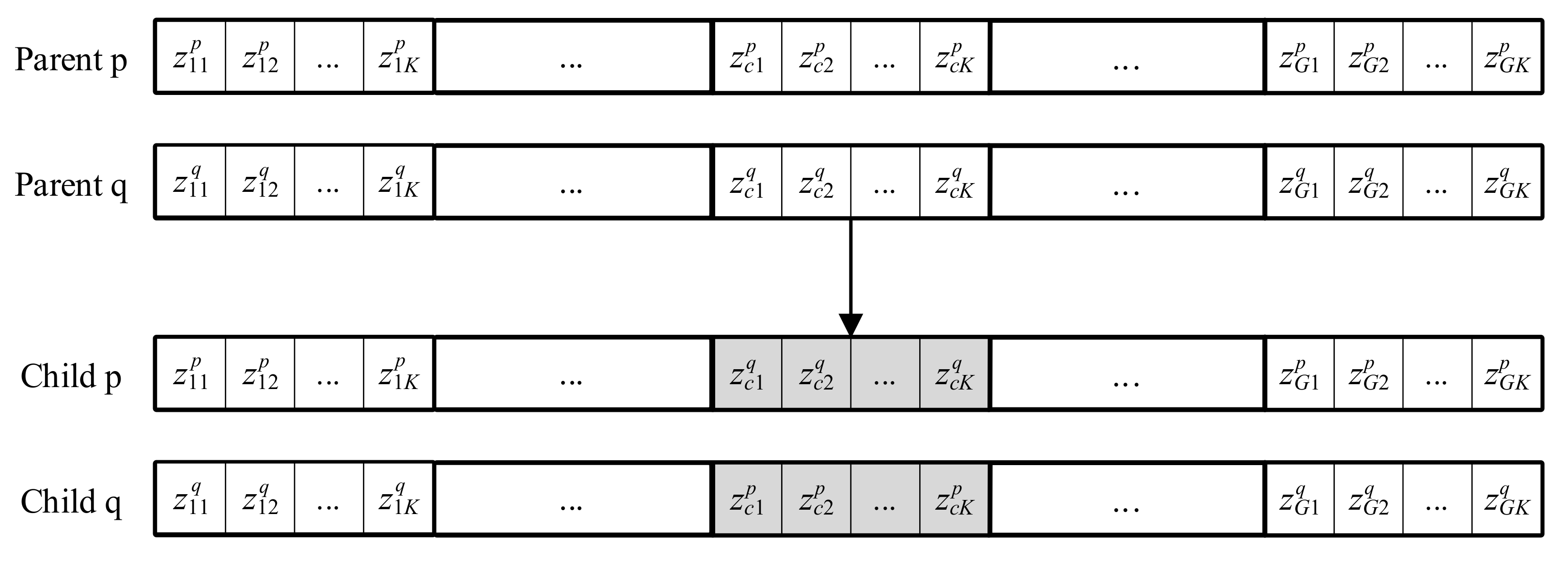
First, we generate a random number α in the interval [0, 1] and compare it with the crossover probability P c . The crossover operator is applied to two parents that are selected randomly to generate two new children while α < P c . We use a single-point crossover operator, and the crossover point is selected based on a random integer c 1 , G . The crossover process is shown in Figure 3.
(3)
Mutation operator
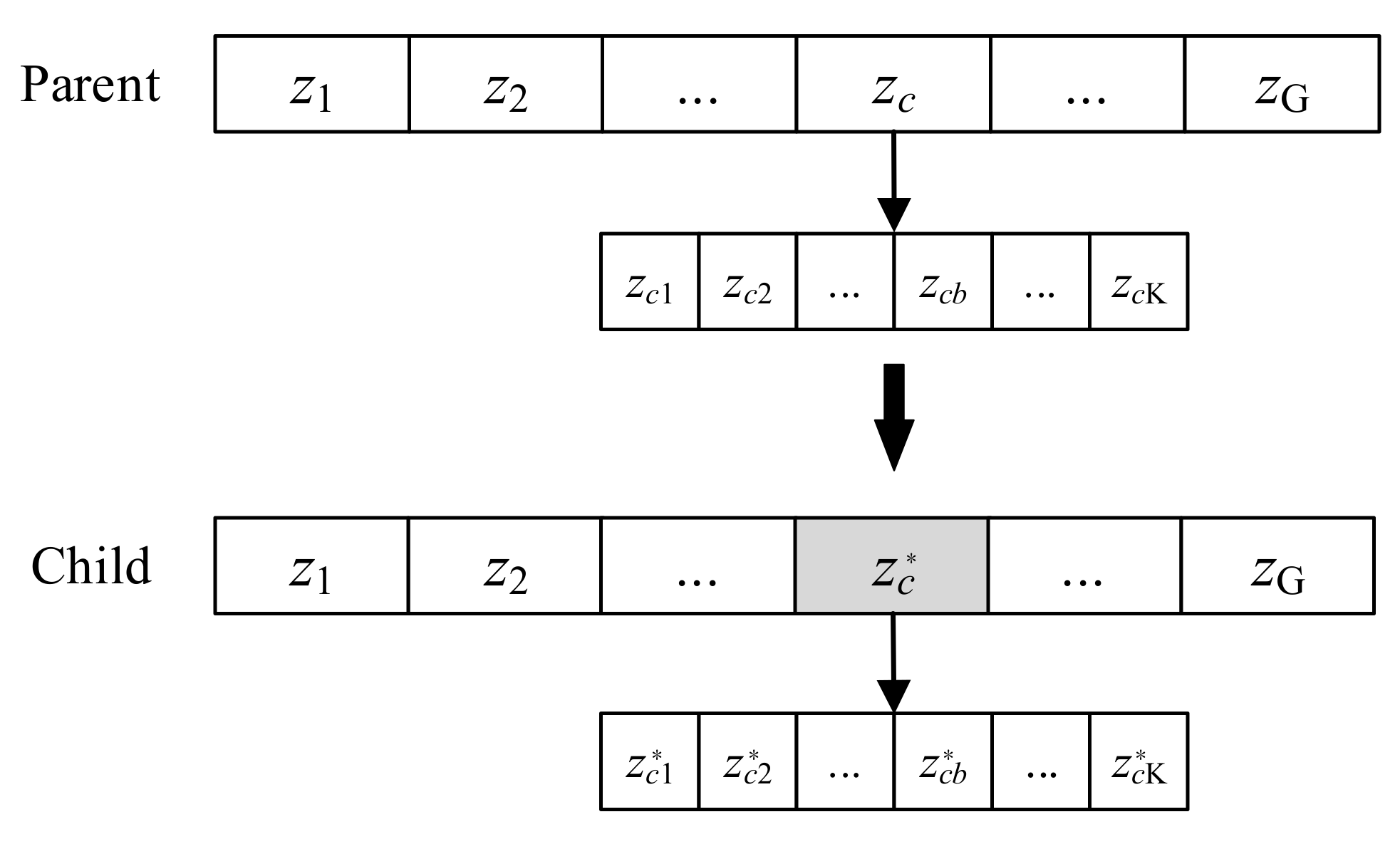
For each individual, we generate a random value β in the interval   0 ,   1 and compare it to the mutation probability P m . If β < P m , we mutate that individual using a single-point mutation one by replacing randomly selected gene with a new random K-dimensional center Z c *   z c 1 * , z c 2 * , , z c K * , as shown in Figure 4.
(4)
Steps of FCM-based GA
The following steps must be implemented to apply the proposed FCM-based GA.
Step 1: Set the parameter values, namely the number of clusters G , number of generations G N , population size P S , crossover probability P c , mutation probability P m , fuzziness value m , and termination tolerance ε .
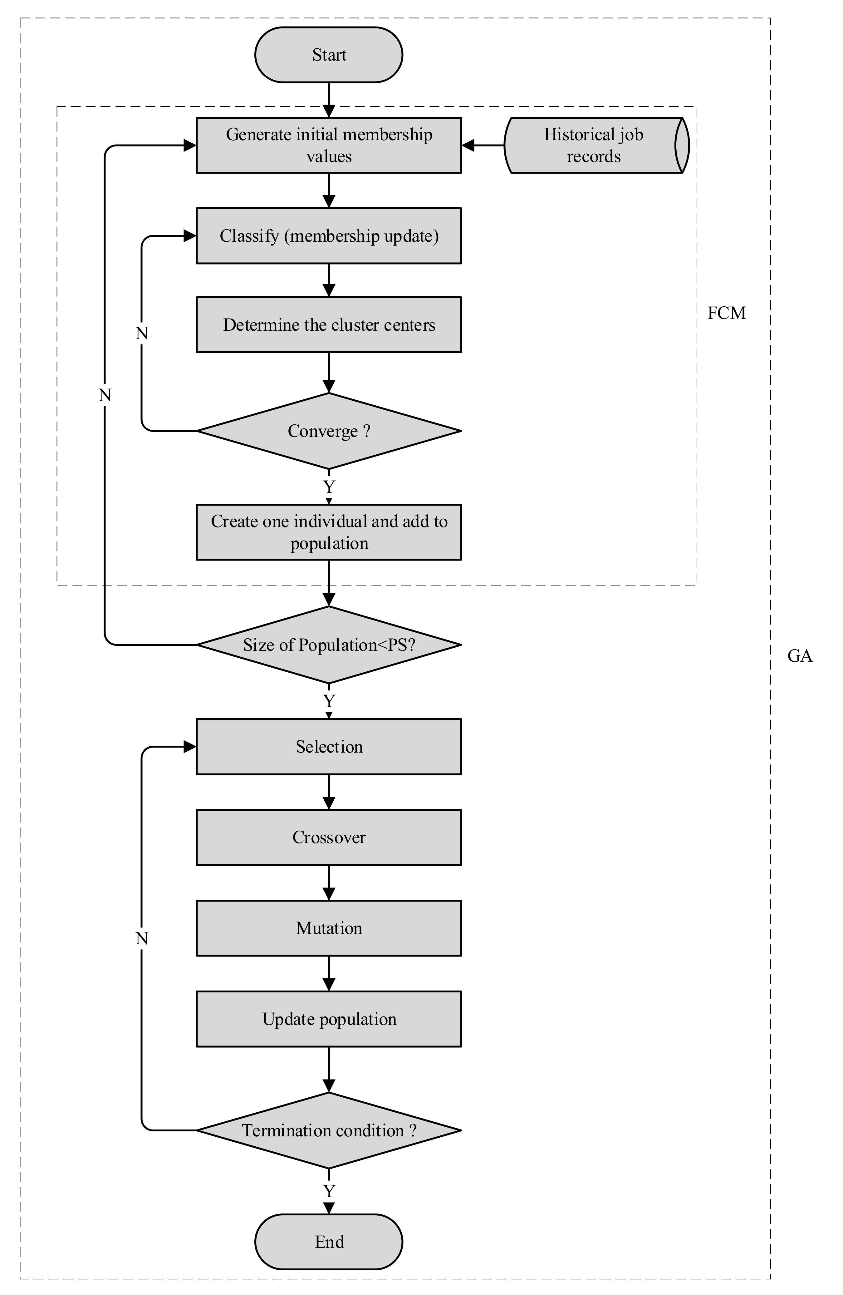
Step 2: Initialize the population. Chromosomes are generated using the FCM clustering methods as many times as P S . To produce a chromosome, we calculate the membership value u i c for each job record i to each cluster c by randomly generated numbers γ i c , 0 γ i c 1 , as follows
u i c = γ i c / c G γ i c .
Step 3: Apply genetic operations. The value of the fitness function   F (Equation (7)) can be calculated for each individual. We then use genetic operations, namely the selection, crossover, and mutation operators, to improve population diversity.
Step 4: Apply optimal preservation. For each generation, the fitness values are re-calculated after the genetic operations have been applied to evaluate each individual. Individuals with higher fitness values are more likely to be chosen for survival.
Step 5: Check termination condition. In the present study, the iteration terminates either after a given number of generations G N or when a given fitness variance value ε is achieved. If either of these conditions is satisfied, then evolution stops. Otherwise, we return to step 3. For a population of P S , indexed by p , the variance ε is calculated as
ε = p = 1 P S F p p = 1 P S F p P S 2 .
After the evolution process is complete, we can obtain the K-dimensional center for each cluster and the membership values. We then associate each job record to all clusters only if its membership value u i c exceeds a given threshold value δ . An auxiliary binary variable ϵ i c is used to calculate the expected job cycle time for all clusters. Finally, the expected job cycle time in each cluster c can be calculated as
e t c = i R u i c · c t i · ϵ i c i R u i c · ϵ i c ,
where ,   ϵ i c = 1           if   u i c > δ   0           otherwise .
Figure 5 shows a flowchart of the complete FCM-based GA approach.

2.4. Backpropagation Network (BPN) Predictor

After the classification is complete, the K-dimensional center for each cluster and the corresponding expected job cycle time is obtained. This information represents the overall behavior and relationship of the dataset. It is important to determine the number of clusters required to capture the most information from the dataset. With too few clusters, it is hard to identify the main features of the dataset. Meanwhile, with too many clusters, the locations of the cluster centers are easily affected by some isolated and noisy job records. Therefore, we test multiple clusters to identify the best combination of experimental parameters and numbers of clusters in the next section.
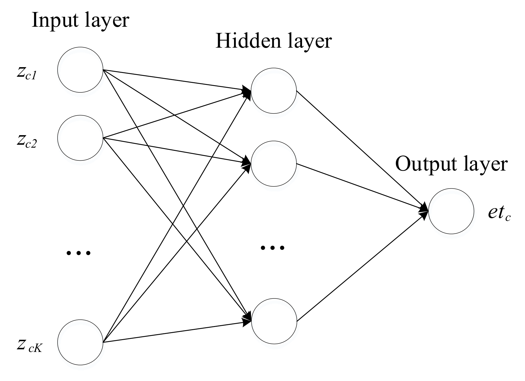
For the cluster centers, the relationship between the independent variables (or attributes) and the corresponding job cycle time has been shown to be nonlinear [23]. As illustrated in Section 2, BPNs are well-known tools for fitting nonlinear relationships. In this sense, a BPN is a good choice for fitting the relationship and predicting the job cycle time [57,58]. Law [59] emphasized that the results predicted by BPNs are accurate with relatively few errors because a BPN adjusts its weights in the output layer to model the training elements. A BPN compares its output with the actual values and propagates the error back through the network. This process is repeated until the error falls within the range of acceptance, whereupon the neural network has been trained successfully. However, determining suitable training and architectural parameters remains difficult. These parameters are usually determined either by trial and error or by pairwise comparisons. The main structure of our BPN is shown in Figure 6.
Since there is no standard method to construct the BPNs for certain problems [20], we have tested several structures of BPNs on a trial-and-error basis. BPN has a stronger nonlinear mapping ability and flexible network structure. Additionally, the hidden layer may be one or more depending upon the complexity of the problem. More hidden layers might result in overfitting. In this sense, this study uses BPN with one hidden layer rather than ANN for fitting nonlinear relationships between the attribute values and job cycle time. Besides, one hidden layer is used for faster convergence without losing much quality.
The BPN usually consists of at least three layers. Each layer contains many neurons, and the neurons in adjacent layers are interconnected by a set of weights. Here, the detailed configuration and training information of BPN are described as follows:
(1) Input layer There are G cluster centers, each with K attributes. Therefore, K neurons are set in the input layer. The G cluster centers with K attribute values and the expected job cycle time are normalized to fall within the interval 0 ,   1 , indexed by τ c b , according to
τ c b = z c b min v R b max v R b min v R b .
(2) Single hidden layer The hidden layer may be one or more depends upon the complexity of the problem. In this study, one hidden layer is used for faster convergence and avoiding overfitting without losing much quality.
(3) Output layer The predicted job cycle time is obtained in normalized form.
(4) Training method Gradient descent has been used as a training method in this study since it is the most commonly used.
(5) Activation/transformation function We use the following nonlinear sigmoid function [60] as the activation function:
f x = 1 1 + e x ,
where x is a random variable.
(6) Learning rate ( π ): 0.01–1.0.
(7) Convergence criterion Many measures can be used to determine when to cease BPN training. Here, the following formula is used in the BPN:
T error = c = 1 G e t c e t ^ c 2 2 ,
where e t ^ c is the job cycle time of cluster c, which is calculated at the output layer using the set of currently trained weights. The BPN training stops when T error falls below 10 3 .

3. Computational Results

3.1. Data Description

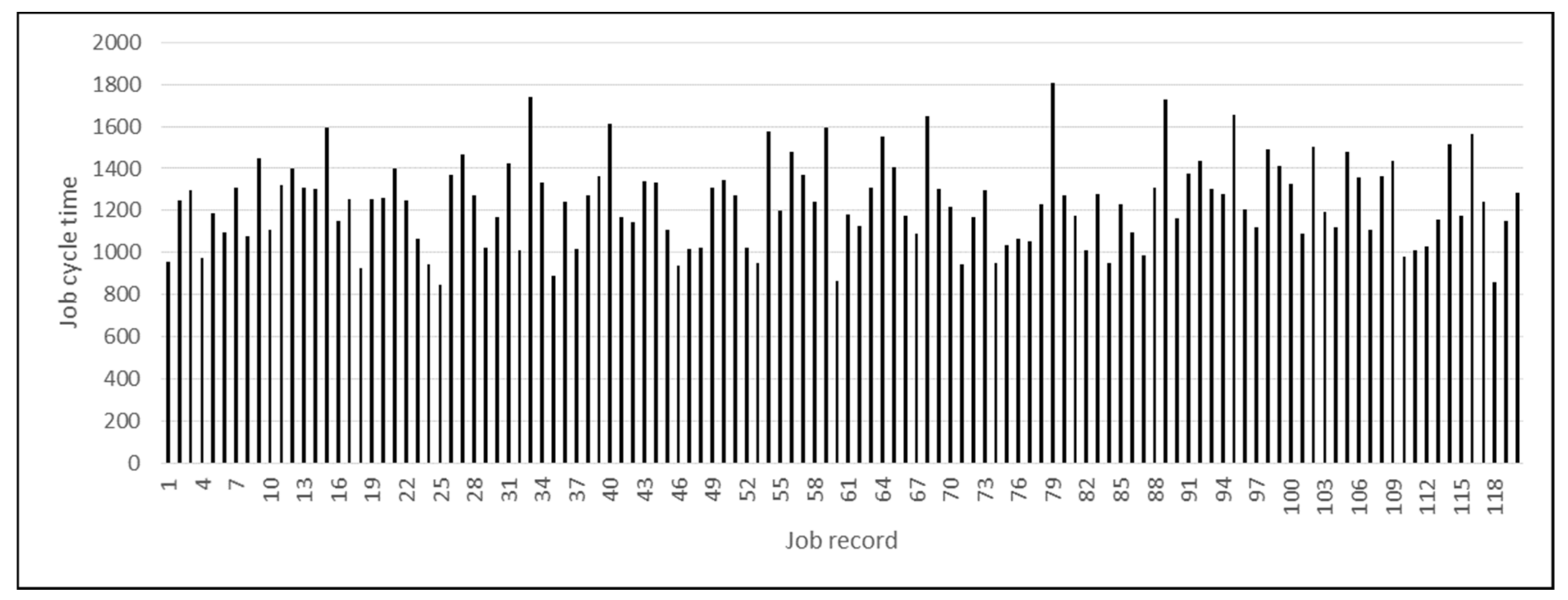
To demonstrate how the proposed approach is applied, we use a series of 120 job records used in the previous research [51,58]. They were collected from a wafer fabrication factory and are shown in Figure 7. The unit of job cycle time is given by hour (h). The job cycle time has an average of 1237 h and a standard deviation of 205 h. The job cycle time pattern is highly nonstationary and is not stable. Additionally, the job cycle time is correlated strongly with six attribute variables, as mentioned in the Methodology section. To demonstrate and evaluate the predictive performance of the proposed approach and assess its accuracy fairly, we split these 120 job records into two datasets, namely (i) training dataset and (ii) testing dataset. Since the dataset used for testing usually accounts for a small proportion of the whole dataset, in this study, the first 110 job records are used for (i) the first 110 job records for clustering and training and (ii) the remaining 10 job records for testing.

3.2. Experimental Settings

The FCM-based GA is used to classify the first 110 job records into G clusters. The obtained cluster centers are fed into the BPN. After learning and training, 10 new testing jobs are given to the trained BPN predictor to predict their cycle times, where the prediction performance is assessed in terms of the mean absolute error (MAE), mean absolute percentage error (MAPE), and root-mean-squared error (RMSE), which are calculated as
MAE = n = 1 N Y n Y ^ n N ,
MAPE = n = 1 N Y n Y ^ n N · Y i ,
RMSE = n = 1 N Y n Y ^ n 2 N ,
where Y n Y ^ n is the absolute difference between the predicted and observed values.
Many parameters affect the accuracy of the job cycle time prediction. Herein, we test the performance and compare the results by using different cluster numbers   G , different neuron numbers ξ in the hidden layer, and different threshold values δ . In addition, all experiments are conducted using populations with the same number of individuals. The remaining parameters used for the FCM-based GA and BPN are summarized in Table 1.
We implement the proposed hybrid approach in C++ using Visual Studio 2013. The experiments are run on a computer with an Intel Core i7-4790 CPU @3.6 GHz and 16 GB of memory under Windows 10 Professional edition. Because the BPN performance is sensitive to the initial conditions of random weights [39], the experiment is repeated at least five times with different initial conditions. The best and average predicted values are recorded for subsequent analysis.

3.3. Experimental Results

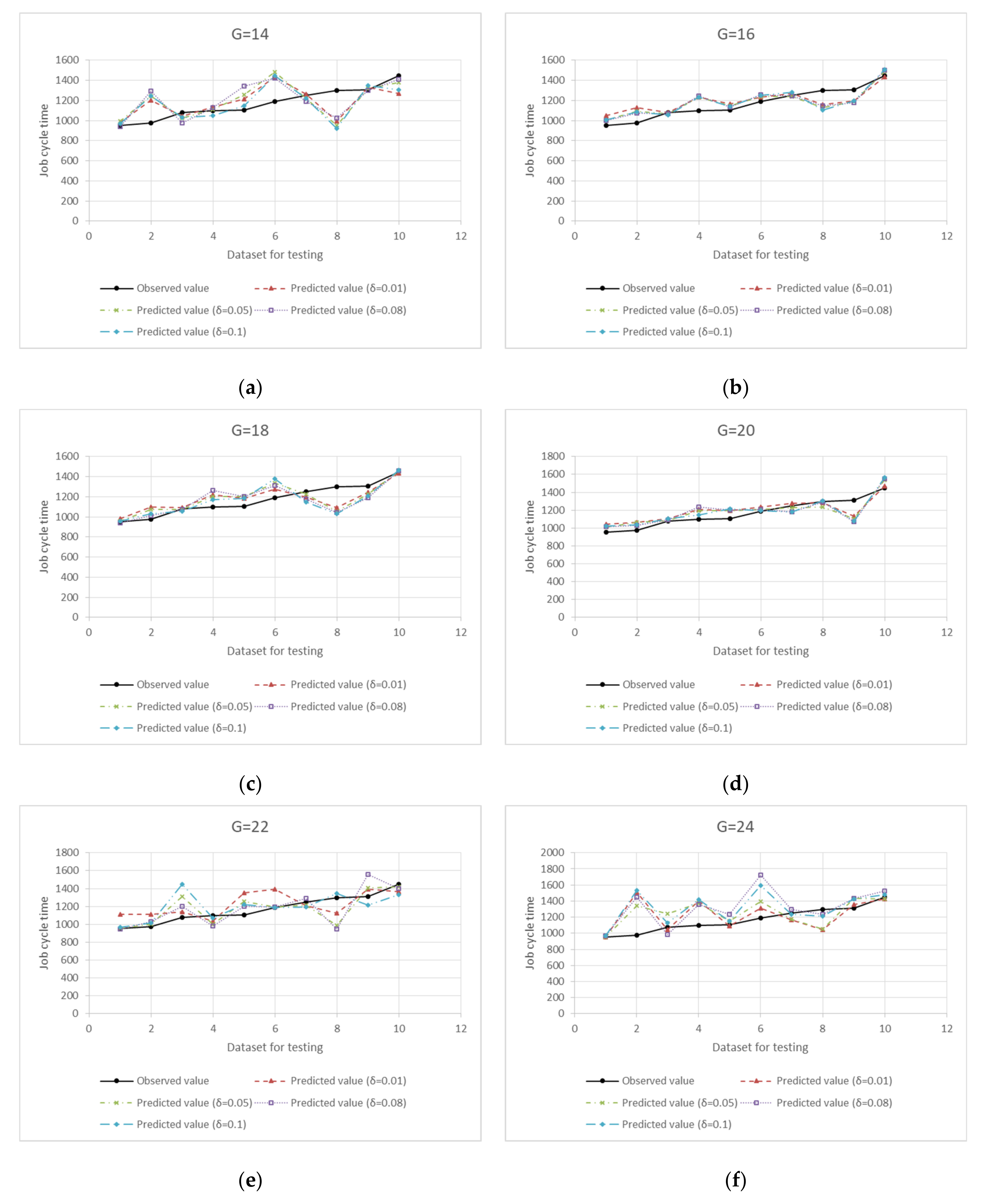
The predicted job cycle times and the observed job cycle times for different numbers of clusters and different membership threshold values are presented in Figure 8. It shows that the predicted job cycle time follows similar patterns to those of the observed data. The proposed approach is quite effective in predicting the job cycle time, and computational results show that the observed and predicted job cycle times are matched well when the number of clusters goes from 16 to 20.
Note that the membership threshold value may indeed affect the accuracy of the job cycle time prediction. As the number of clusters increases from 20 to 24, the job cycle time prediction performance fluctuates more under different membership threshold values. Next, we discuss the job cycle time prediction accuracy in terms of the MAE (hours), MAPE (%), and RMSE (hours).
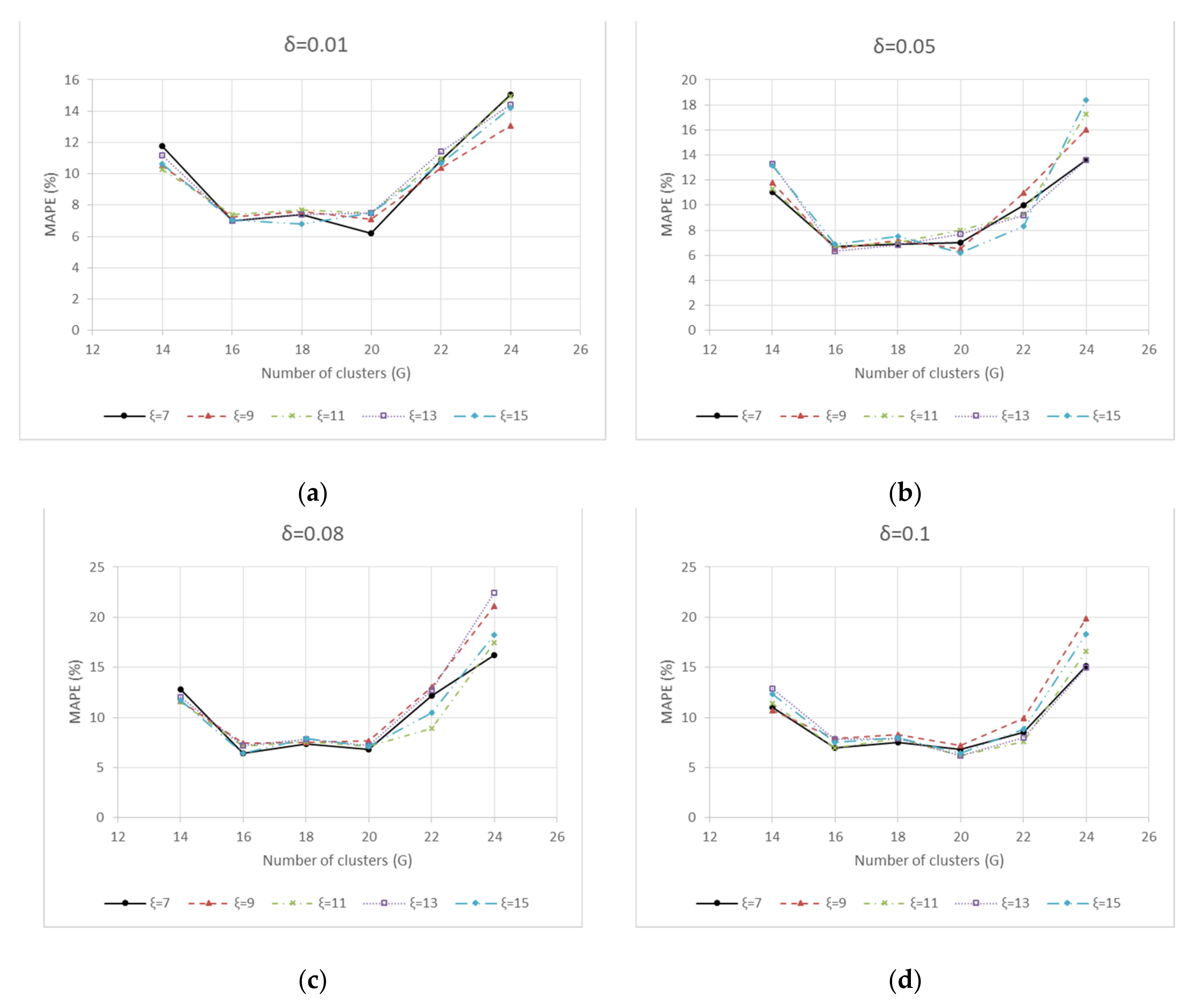
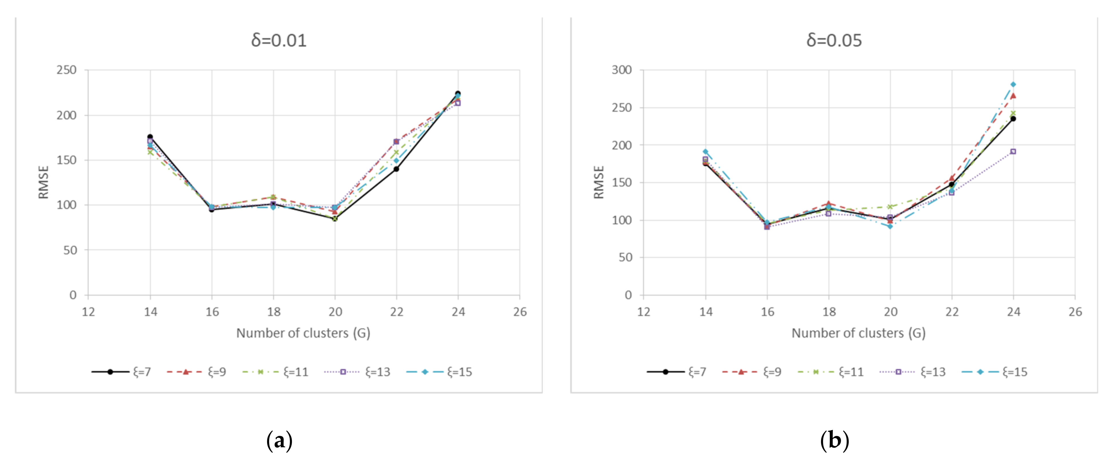
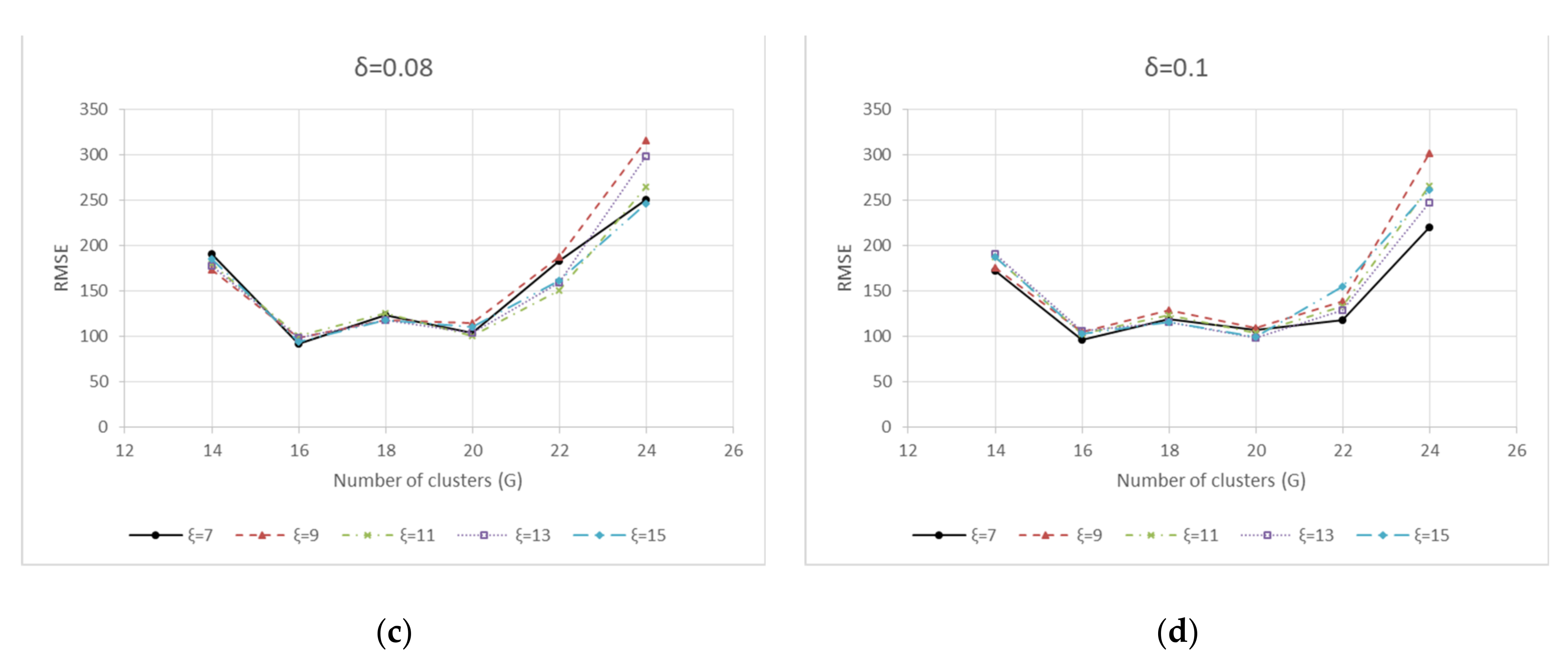
To investigate how the number of clusters affects the prediction accuracy, we experimented using six different numbers of clusters, namely 14, 16, 18, 20, 22, and 24. The MAE, MAPE, and RMSE are used to evaluate the effects of the number of clusters overall testing data for the identical threshold value and the identical number of neurons in the BPN hidden layer, in Figure 9, Figure 10 and Figure 11, respectively. These figures show similar trends in the MAE, MAPE, and RMSE values against different numbers of clusters, indicating that there might be the need to study optimal numbers of clusters appropriate to datasets but beyond the scope of this study. The curves of MAE, MAPE, and RMSE show that the job cycle time prediction accuracy is strongly correlated with the number of clusters. The job cycle time prediction performance varies with the number of clusters and is poor with too many or too few clusters, meaning that increasing or decreasing the number of clusters does not provide better job cycle time predictions.
In Figure 9, we generally obtain better job cycle time prediction performance (MAE) with the threshold values δ = 0.05   or   0.08 . These threshold values provide good data classification that improves the job cycle time prediction accuracy in the BPN predictor. Similar trends are obtained for the MAPE and RMSE values in Figure 10 and Figure 11, respectively.
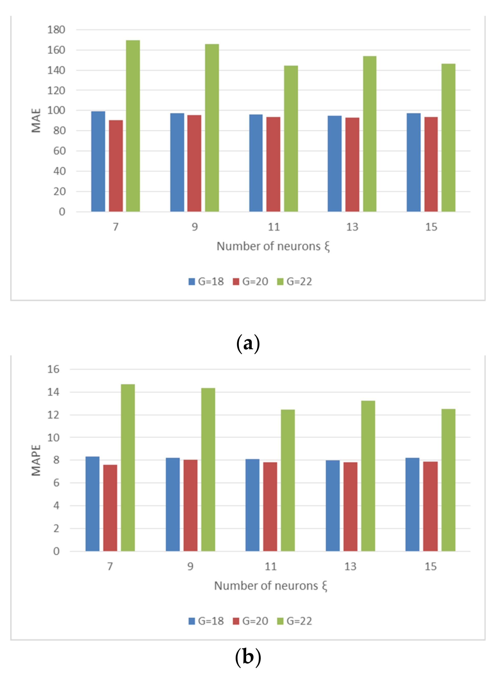
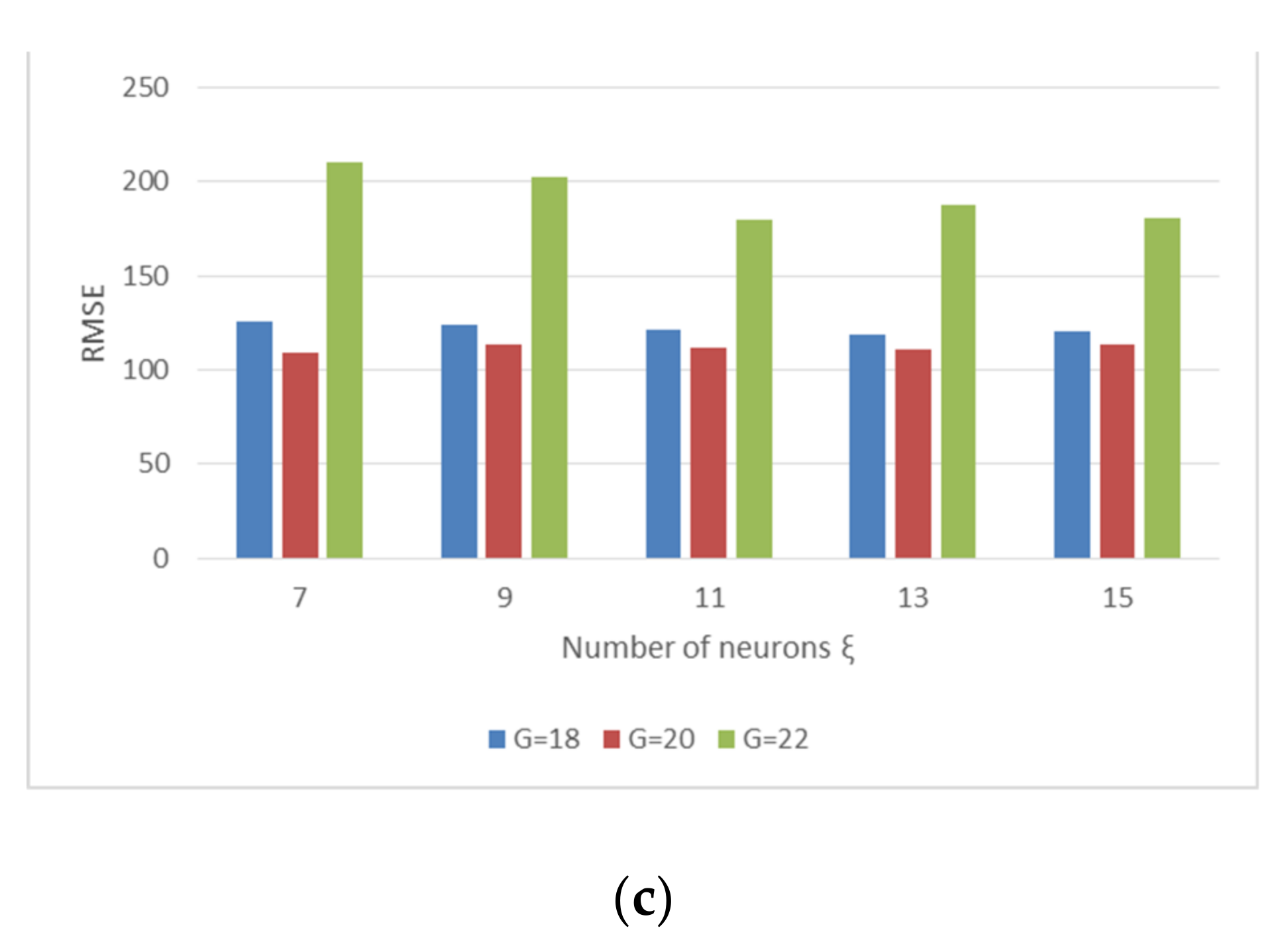
To investigate the effect of different numbers of neurons in the BPN hidden layer, we test the job cycle time prediction performance with the identical numbers of clusters (18, 20, and 22) by taking the average MAE, MAPE, and RMSE values for five runs and four threshold values, as shown in Figure 12. The job cycle time prediction performance is clearly not strongly correlated with the number of neurons in the hidden layer of the BPN predictor: increasing the number of neurons ξ improves the prediction accuracy only marginally.
Table 2 summarizes the prediction performance, where the best and average MAE, MAPE, and RMSE values are recorded for five experiment runs with three different numbers of clusters (18, 20, and 22), five different numbers of neurons in the hidden layer (7, 9, 11, 13, and 15) and four different threshold value δ (0.01, 0.05, 0.08 and 0.1).
Since the performance measures (MAE, MAPE, and RMSE) are about the prediction errors, the best prediction results were obtained are shaded grey in Table 2 when G = 20 , δ = 0.01 , and ξ = 7 . Furthermore, to evaluate the effectiveness and efficiency of the proposed hybrid approach, we compare with five existing approaches that were implemented for the same dataset as ours in previous works (Chen 2007b, Chen 2016b); they are (i) linear regression (LR), (ii) BPN, (iii) k-means BPN, (iv) k-means fuzzy BPN [36], and (v) post-classification BPN (Chen [58]).
In Table 3, the best prediction results obtained with the proposed approach with G = 20 , δ = 0.01 , and ξ = 7 are compared with those of the five existing approaches. The best results in the previous research were obtained by post-classification BPN (Chen 2016b). The comparison for MAE was made through the following equation. For MAPE and RMSE, similar calculations have been performed to calculate the improvements over the best-known methods.
Improvement   % = MAE best   known   method MAE proposed   method MAE best   known   method ,
As shown in Table 3, the prediction accuracies are improved by 16.3%, 4.6%, and 19.6% as measured in terms of MAE, MAPE, and RMSE, respectively. Comparing the proposed approach with the previous ones in Table 3 suggests that the former is effective and applicable. It is also clear that the classification-based hybrid approaches (k-means BPN, k-means fuzzy BPN, post-classification BPN, and the proposed approach) perform better than the other approaches (LR and BPN). The proposed hybrid approach is better than other BPNs because it is challenging to train the BPN using raw job records because of the overfitting problem. The proposed approach is better than the k-means fuzzy BPN approach because a better classification is obtained using the FCM-based GA method.

4. Conclusions

This study investigated the relationships between job attributes and job cycle time using a dataset obtained from a semiconductor fabrication factory. To enhance the effectiveness of the job cycle time prediction for semiconductor fabrication factories, a new hybrid approach is proposed, and it comprises FCM-based GA and BPN. Many previous studies used pre-classification or post-classification methods. However, such methods have several drawbacks, such as unequal sizes of different clusters. The FCM-based GA represents a new soft unsupervised classification method wherein the GA is used to improve the classification performance of the FCM. Hence, a good set of cluster centers are obtained while balancing the fuzzy memberships of data points to different centers by applying the FCM-based GA, which captures the main features of the dataset. The results obtained from the FCM-based GA are used as the training data and fed into the BPN predictor. The BPN predictor is then trained to predict the cycle time of new jobs with different attributes.
We also presented a case study to demonstrate the effectiveness of the proposed approach. To obtain good job cycle time prediction performance, various parameters in the experiments were tested to achieve the best performance. The obtained results were compared to those of the previous research to show the dominating performance over the existing methodologies. These efforts lead us to the following conclusions: (1) The FCM-based GA can better pre-classify the first dataset of job records, enabling the BPN to produce accurate job cycle time predictions; (2) Stable and fuzzy job-record classification results allow the BPN to predict the job cycle time more accurately, as shown in Table 3; (3) The proposed hybrid approach indicates that classification-based methods are superior to those without job-record classification.
The limitation of this study is explained here. The computational times were not obtained during the experiments since most studies using the single-layer ANN with the back propagation do not measure it meaningfully. More precisely, the computational times can be divided into (1) FCM clustering and GA, and (2) ANN training. The prediction time is almost instant. The computational times for FCM clustering and GA were varied by various parameters, including the number of centers, threshold values, and many GA parameters (shown in Table 1), which requires significant efforts in the design of experiments to optimize the performance. The training time depends on the size of the data and the training algorithm. Since the primary focus of this study was to propose a novel algorithm, the experimental design to understand the performance is beyond this study.
Another limitation is also related to the optimization of the performance. A simple train/test split was used instead of k-fold cross-validation, which may help the best performance of the ANN training. The primary reason is why the goal of this study was to propose a novel methodology, not to optimize the proposed algorithms. In addition, since FCM clustering is used, we believe that its effects may be aggregated as a grouping in k-fold cross-validation. Furthermore, since we used the clustered c-means by the stochastic algorithm (i.e., GA) instead of the raw data, the benefits of the resampling by k-fold cross-validation may not be justified. However, the study on the benefits of the k-fold cross-validation in our proposed algorithm can be studied in the future.
In future work, we plan to explore the following interesting problems. The optimal number of clusters can be identified by further research of preprocessing the dataset. Given their importance, the proposed approach could be modified to predict the lower and upper job cycle time bounds. In addition, fuzzy concepts could be incorporated into the BPN to enhance prediction accuracy. Another interesting direction for future work would be identifying and eliminating invalid job records because such noise data may affect prediction accuracy. All these questions are considered in future research.

Author Contributions

Conceptualization, G.M.L., X.G.; Formal analysis, G.M.L.; Funding acquisition, G.M.L.; Methodology, X.G.; Project administration G.M.L.; Supervision, G.M.L.; Validation, G.M.L.; Writing—original draft, X.G.; Writing—review & editing, G.M.L. Both authors have read and agreed to the published version of the manuscript.

Funding

This work was supported by the National Research Foundation of Korea (NRF) grant funded by the Korea government (MSIT) (No. 2018R1A2B3008890).

Institutional Review Board Statement

Not applicable.

Informed Consent Statement

Not applicable.

Data Availability Statement

Not applicable.

Conflicts of Interest

The authors declare no conflict of interest.

References

  1. Chang, P.-C.; Hsieh, J.-C.; Liao, T.W. A case-based reasoning approach for due-date assignment in a wafer fabrication factory. In Proceedings of the International Conference on Case-Based Reasoning (ICCBR 2001), Vancouver, BC, Canada, 30 July–2 August 2001; pp. 648–659. [Google Scholar]
  2. Chen, T. A fuzzy back propagation network for output time prediction in a wafer fab. Appl. Soft Comput. 2003, 2, 211–222. [Google Scholar] [CrossRef]
  3. Kulkarni, V.; Nicola, V.; Smith, R.; Trivedi, K. Numerical Evaluation of Performability and Job Completion Time in Repairable Fault-tolerant Systems. In Proceedings of the 16th Intl. Symp. on Fault Tolerant Computing, Vienna, Austria, 1–4 July 1986. [Google Scholar]
  4. Mehrotra, K.; Chai, J.; Pillutla, S. A study of approximating the moments of the job completion time in PERT networks. J. Oper. Manag. 1996, 14, 277–289. [Google Scholar] [CrossRef]
  5. Chen, T. Job cycle time estimation in a wafer fabrication factory with a bi-directional classifying fuzzy-neural approach. Int. J. Adv. Manuf. Technol. 2011, 56, 1007–1018. [Google Scholar] [CrossRef]
  6. Chen, T.; Romanowski, R. Precise and accurate job cycle time forecasting in a wafer fabrication factory with a fuzzy data mining approach. Math. Probl. Eng. 2013, 2013. [Google Scholar] [CrossRef]
  7. Glassey, C.R.; Resende, M.G. Closed-loop job release control for VLSI circuit manufacturing. IEEE Trans. Semicond. Manuf. 1988, 1, 36–46. [Google Scholar] [CrossRef]
  8. Pai, P.-F.; Lee, C.-E.; Su, T.-H. A daily production model for wafer fabrication. Int. J. Adv. Manuf. Technol. 2004, 23, 58–63. [Google Scholar] [CrossRef]
  9. Chen, T. A fuzzy-neural approach for estimating the monthly output of a semiconductor manufacturing factory. Int. J. Adv. Manuf. Technol. 2008, 39, 589–598. [Google Scholar] [CrossRef]
  10. Wang, J.; Zhang, J. Big data analytics for forecasting cycle time in semiconductor wafer fabrication system. Int. J. Prod. Res. 2016, 54, 7231–7244. [Google Scholar] [CrossRef]
  11. Chung, S.-H.; Huang, H.-W. Cycle time estimation for wafer fab with engineering lots. Iie Trans. 2002, 34, 105–118. [Google Scholar] [CrossRef]
  12. Raddon, A.; Grigsby, B. Throughput time forecasting model. In Proceedings of the 1997 IEEE/SEMI Advanced Semiconductor Manufacturing Conference and Workshop ASMC 97 Proceedings, Cambridge, MA, USA, 10–12 September 1997; pp. 430–433. [Google Scholar]
  13. Backus, P.; Janakiram, M.; Mowzoon, S.; Runger, C.; Bhargava, A. Factory cycle-time prediction with a data-mining approach. IEEE Trans. Semicond. Manuf. 2006, 19, 252–258. [Google Scholar] [CrossRef]
  14. Yang, F.; Ankenman, B.; Nelson, B.L. Efficient generation of cycle time-throughput curves through simulation and metamodeling. Nav. Res. Logist. (NRL) 2007, 54, 78–93. [Google Scholar] [CrossRef]
  15. Yang, F.; Ankenman, B.E.; Nelson, B.L. Estimating cycle time percentile curves for manufacturing systems via simulation. INFORMS J. Comput. 2008, 20, 628–643. [Google Scholar] [CrossRef]
  16. Pearn, W.; Chung, S.; Lai, C. Due-date assignment for wafer fabrication under demand variate environment. IEEE Trans. Semicond. Manuf. 2007, 20, 165–175. [Google Scholar] [CrossRef]
  17. Tai, Y.; Pearn, W.; Lee, J. Cycle time estimation for semiconductor final testing processes with Weibull-distributed waiting time. Int. J. Prod. Res. 2012, 50, 581–592. [Google Scholar] [CrossRef]
  18. Shanthikumar, J.G.; Ding, S.; Zhang, M.T. Queueing theory for semiconductor manufacturing systems: A survey and open problems. IEEE Trans. Autom. Sci. Eng. 2007, 4, 513–522. [Google Scholar] [CrossRef]
  19. Morrison, J.R.; Martin, D.P. Practical extensions to cycle time approximations for the G/G/m-queue with applications. IEEE Trans. Autom. Sci. Eng. 2007, 4, 523–532. [Google Scholar] [CrossRef]
  20. Singh, A.; Das, A.; Bera, U.K.; Lee, G.M. Prediction of transportation costs using trapezoidal neutrosophic fuzzy analytic hierarchy process and artificial neural networks. IEEE Access 2021, 9, 103497–103512. [Google Scholar] [CrossRef]
  21. Chang, P.C.; Hsieh, J.C. A neural networks approach for due-date assignment in a wafer fabrication factory. Int. J. Ind. Eng. 2003, 10, 55–61. [Google Scholar]
  22. Sha, D.Y.; Hsu, S.Y. Due-date assignment in wafer fabrication using artificial neural networks. Int. J. Adv. Manuf. Technol. 2004, 23, 768–775. [Google Scholar] [CrossRef]
  23. Chien, C.-F.; Hsu, C.-Y.; Hsiao, C.-W. Manufacturing intelligence to forecast and reduce semiconductor cycle time. J. Intell. Manuf. 2012, 23, 2281–2294. [Google Scholar] [CrossRef]
  24. Gazder, U.; Ratrout, N.T. A new logit—Artificial neural network ensemble for mode choice modeling: A case study for border transport. J. Adv. Transp. 2016, 49, 855–866. [Google Scholar] [CrossRef]
  25. Chiu, C.; Chang, P.-C.; Chiu, N.-H. A case-based expert support system for due-date assignment in a wafer fabrication factory. J. Intell. Manuf. 2003, 14, 287–296. [Google Scholar] [CrossRef]
  26. Chang, P.-C.; Fan, C.Y.; Wang, Y.-W. Evolving CBR and data segmentation by SOM for flow time prediction in semiconductor manufacturing factory. J. Intell. Manuf. 2009, 20, 421. [Google Scholar] [CrossRef]
  27. Liu, C.-H.; Chang, P.-C.; Kao, I.-W. Cluster based evolving FCBR for flow time prediction in semiconductor manufacturing factory. In Proceedings of the 8th WSEAS International Conference on Applied Computer Science (ACS’08), Venice, Italy, 21–23 November 2008; pp. 424–429. [Google Scholar]
  28. Vig, M.M.; Dooley, K.J. Dynamic rules for due-date assignment. Int. J. Prod. Res. 1991, 29, 1361–1377. [Google Scholar] [CrossRef]
  29. Veeger, C.; Etman, L.; Lefeber, E.; Adan, I.; Van Herk, J.; Rooda, J. Predicting cycle time distributions for integrated processing workstations: An aggregate modeling approach. IEEE Trans. Semicond. Manuf. 2011, 24, 223–236. [Google Scholar] [CrossRef] [Green Version]
  30. Hsieh, L.Y.; Chang, K.-H.; Chien, C.-F. Efficient development of cycle time response surfaces using progressive simulation metamodeling. Int. J. Prod. Res. 2014, 52, 3097–3109. [Google Scholar] [CrossRef]
  31. Yang, D.; Hu, L.; Qian, Y. Due Date Assignment in a Dynamic Job Shop with the Orthogonal Kernel Least Squares Algorithm. In IOP Conference Series: Materials Science and Engineering; IOP Publishing: Bristol, UK, 2017; Volume 212. [Google Scholar]
  32. Chang, P.-C.; Hieh, J.-C.; Liao, T.W. Evolving fuzzy rules for due-date assignment problem in semiconductor manufacturing factory. J. Intell. Manuf. 2005, 16, 549–557. [Google Scholar] [CrossRef]
  33. Chen, T. Fuzzy-neural-network-based fluctuation smoothing rule for reducing the cycle times of jobs with various priorities in a wafer fabrication plant: A simulation study. J. Eng. Manuf. 2009, 223, 1033–1043. [Google Scholar] [CrossRef]
  34. Gao, X.; Zhou, Y.; Amir, M.I.H.; Rosyidah, F.A.; Lee, G.M. A hybrid genetic algorithm for multi-emergency medical service center location-allocation problem in disaster response. Int. J. Ind. Eng. Theory Appl. Pract. 2017, 24, 663–679. [Google Scholar]
  35. Gao, X.; Lee, G.M. Moment-based Rental Prediction for Bicycle-sharing Transportation Systems Using a Hybrid Genetic Algorithm and Machine Learning. Comput. Ind. Eng. 2019, 128, 60–69. [Google Scholar] [CrossRef]
  36. Chen, T. An intelligent hybrid system for wafer lot output time prediction. Adv. Eng. Inform. 2007, 21, 55–65. [Google Scholar] [CrossRef]
  37. Chen, T.; Wu, H.-C.; Wang, Y.-C. Fuzzy-neural approaches with example post-classification for estimating job cycle time in a wafer fab. Appl. Soft Comput. 2009, 9, 1225–1231. [Google Scholar] [CrossRef]
  38. Tirkel, I. Cycle time prediction in wafer fabrication line by applying data mining methods. In Proceedings of the 2011 IEEE/SEMI Advanced Semiconductor Manufacturing Conference, Saratoga Springs, NY, USA, 16–18 May 2011; pp. 1–5. [Google Scholar]
  39. Chen, T.; Lin, Y.-C. A fuzzy back propagation network ensemble with example classification for lot output time prediction in a wafer fab. Appl. Soft Comput. 2009, 9, 658–666. [Google Scholar] [CrossRef]
  40. Chen, T. Asymmetric cycle time bounding in semiconductor manufacturing: An efficient and effective back-propagation-network-based method. Oper. Res. 2016, 16, 445–468. [Google Scholar] [CrossRef]
  41. Chen, T.; Wang, Y.-C. A nonlinearly normalized back propagation network and cloud computing approach for determining cycle time allowance during wafer fabrication. Robot. Comput. Integr. Manuf. 2017, 45, 144–156. [Google Scholar] [CrossRef]
  42. Yokota, T.; Gen, M.; Li, Y.-X. Genetic algorithm for non-linear mixed integer programming problems and its applications. Comput. Ind. Eng. 1996, 30, 905–917. [Google Scholar] [CrossRef]
  43. Yu, X.; Gen, M. Introduction to Evolutionary Algorithms; Springer: London, UK, 2010. [Google Scholar]
  44. Chen, T. Incorporating fuzzy c-means and a back-propagation network ensemble to job completion time prediction in a semiconductor fabrication factory. Fuzzy Sets Syst. 2007, 158, 2153–2168. [Google Scholar] [CrossRef]
  45. Chen, T. A job-classifying and data-mining approach for estimating job cycle time in a wafer fabrication factory. Int. J. Adv. Manuf. Technol. 2012, 62, 317–328. [Google Scholar] [CrossRef]
  46. Chen, T. A hybrid fuzzy-neural approach to job completion time prediction in a semiconductor fabrication factory. Neurocomputing 2008, 71, 3193–3201. [Google Scholar] [CrossRef]
  47. Sun, B.; Guo, H.; Karimi, H.R.; Ge, Y.; Xiong, S. Prediction of stock index futures prices based on fuzzy sets and multivariate fuzzy time series. Neurocomputing 2015, 151, 1528–1536. [Google Scholar] [CrossRef]
  48. Rezaee, M.J.; Jozmaleki, M.; Valipour, M. Integrating dynamic fuzzy C-means, data envelopment analysis and artificial neural network to online prediction performance of companies in stock exchange. Phys. A Stat. Mech. Its Appl. 2018, 489, 78–93. [Google Scholar] [CrossRef]
  49. Biju, V.; Mythili, P. A genetic algorithm based fuzzy C mean clustering model for segmenting microarray images. Int. J. Comput. Appl. 2012, 52, 42–48. [Google Scholar]
  50. Ding, Y.; Fu, X. Kernel-based fuzzy c-means clustering algorithm based on genetic algorithm. Neurocomputing 2016, 188, 233–238. [Google Scholar] [CrossRef]
  51. Chen, T.; Wu, H.-C. A new cloud computing method for establishing asymmetric cycle time intervals in a wafer fabrication factory. J. Intell. Manuf. 2017, 28, 1095–1107. [Google Scholar] [CrossRef] [Green Version]
  52. Dunn, J.C. A fuzzy relative of the ISODATA process and its use in detecting compact well-separated clusters. J. Cybern. 1973, 3, 32–57. [Google Scholar] [CrossRef]
  53. Bezdek, J.C.; Dunn, J.C. Optimal fuzzy partitions: A heuristic for estimating the parameters in a mixture of normal distributions. IEEE Trans. Comput. 1975, 100, 835–838. [Google Scholar] [CrossRef]
  54. Kenesei, T.; Balasko, B.; Abonyi, J. A MATLAB toolbox and its web based variant for fuzzy cluster analysis. In Proceedings of the 7th International Symposium on Hungarian Researchers on Computational Intelligence, Budapest, Hungary, 24–25 November 2006; pp. 24–25. [Google Scholar]
  55. Wikaisuksakul, S. A multi-objective genetic algorithm with fuzzy c-means for automatic data clustering. Appl. Soft Comput. 2014, 24, 679–691. [Google Scholar] [CrossRef]
  56. Ye, A.-X.; Jin, Y.-X. A fuzzy c-means clustering algorithm based on improved quantum genetic algorithm. Simulation 2016, 9, 227–236. [Google Scholar] [CrossRef]
  57. Chen, T. A systematic cycle time reduction procedure for enhancing the competitiveness and sustainability of a semiconductor manufacturer. Sustainability 2013, 5, 4637–4652. [Google Scholar] [CrossRef] [Green Version]
  58. Chen, T. Estimating job cycle time in a wafer fabrication factory: A novel and effective approach based on post-classification. Appl. Soft Comput. 2016, 40, 558–568. [Google Scholar] [CrossRef]
  59. Law, R. Back-propagation learning in improving the accuracy of neural network-based tourism demand forecasting. Tour. Manag. 2000, 21, 331–340. [Google Scholar] [CrossRef]
  60. Ripley, B.D. Pattern Recognition and Neural Networks; Cambridge University Press: Cambridge, UK, 2007. [Google Scholar]
Figure 1. Example of FCM with notation (G = 3).
Applsci 11 07428 g001
Figure 2. String encoding for cluster centers.
Applsci 11 07428 g002
Figure 3. Generating two new children from two parents via crossover.
Applsci 11 07428 g003
Figure 4. Mutating one individual.
Applsci 11 07428 g004
Figure 5. Flowchart of FCM-based GA.
Applsci 11 07428 g005
Figure 6. Architecture of the BPN.
Applsci 11 07428 g006
Figure 7. Entire dataset of job records.
Applsci 11 07428 g007
Figure 8. Predicted and observed job cycle times (unit: hour) for different numbers of clusters; 14 (a), 16 (b), 18 (c), 20 (d), 22 (e), and 24 (f).
Applsci 11 07428 g008
Figure 9. Mean absolute error (MAE, unit: hour) against the number of clusters for different numbers of neurons ξ for different thereshold values δ ; δ = 0.01 (a), δ = 0.05 (b) δ = 0.08 , (c), and δ = 0.1 (d).
Applsci 11 07428 g009
Figure 10. Mean absolute percentage error (MAPE, unit: %)) against the number of clusters for different numbers of neurons ξ for different thereshold values δ ; δ = 0.01 (a), δ = 0.05 (b) δ = 0.08 , (c), and δ = 0.1 (d).
Applsci 11 07428 g010
Figure 11. Root-mean-squared error (RMSE, unit: hour) against the number of clusters for different numbers of neurons ξ for different thereshold values δ ; δ = 0.01 (a), δ = 0.05 (b) δ = 0.08 , (c), and δ = 0.1 (d).
Applsci 11 07428 g011aApplsci 11 07428 g011b
Figure 12. (a) MAAE (unit: hour), (b) MAPE (unit:%), and (c) RMSE (unit: hour) for different numbers of neurons.
Applsci 11 07428 g012aApplsci 11 07428 g012b
Table 1. Parameters used in the proposed approach.
ParameterValue
Fuzziness exponent ( m )2
FCM termination tolerance ( ϕ ) 10 4
Number of clusters ( G )14, 16, 18, 20, 22, and 24
Population size ( P S )40
Number of generations ( G N ) 1000
Mutation probability ( P m )0.2
Crossover probability ( P c )0.1
Membership threshold value ( δ )0.01, 0.05, 0.08, and 0.1
Fitness variance value ( ε ) 10 4
Learning rate ( π )0.99
Number of neurons in the input layer ( φ )6
Number of neurons in the hidden layer ( ξ )7, 9, 11, 13, and 15
Table 2. Performance of proposed approach in terms of MAE (hours), MAPE, and RMSE (hours).
G . ξ Best ValueAverage Value
δ 0.010.050.080.10.010.050.080.1
187MAE (h)86.0482.3389.5189.9992.14105.5398.87100.27
MAPE (%)7.406.907.407.507.908.808.208.30
RMSE (h)101.67115.76123.37118.79111.55135.14129.99125.45
9MAE (h)88.3086.4189.5399.5193.8693.9995.90106.99
MAPE (%)7.607.207.508.308.207.808.008.90
RMSE (h)108.87122.07117.35128.34112.11124.32127.07132.91
11MAE (h)90.3182.9691.4395.0692.9792.9697.21100.36
MAPE (%)7.707.007.607.908.007.808.108.40
RMSE (h)109.41112.97125.36123.62109.81119.69130.09125.51
13MAE (h)85.3980.5792.9292.8789.0692.1897.22100.81
MAPE (%)7.406.807.807.907.707.708.108.40
RMSE (h)101.04108.55117.95116.12105.12116.75126.01127.03
15MAE (h)78.2289.7695.4895.9892.4393.1199.19103.92
MAPE (%)6.807.507.908.008.007.808.308.70
RMSE (h)97.27118.15117.98115.53110.32120.37125.70127.18
207MAE (h)70.0383.6280.4482.7486.4590.4588.6296.02
MAPE (%)6.207.006.806.807.607.607.407.90
RMSE (h)85.11101.43104.14106.7998.38109.19109.74118.40
9MAE (h)80.5478.4092.9688.3588.3997.8598.1298.65
MAPE (%)7.106.507.707.207.808.208.108.10
RMSE (h)93.0899.15114.90108.94100.88118.48117.35119.08
11MAE (h)86.3696.9883.5576.7790.25100.7497.3685.25
MAPE (%)7.508.007.106.207.908.308.107.00
RMSE (h)84.78117.79100.23104.06100.01120.98119.32108.48
13MAE (h)86.1791.8285.0974.4388.8294.4797.5890.25
MAPE (%)7.507.707.206.207.707.908.207.50
RMSE (h)97.39104.01103.5997.87100.77112.05119.35113.06
15MAE (h)84.9773.2087.9478.0291.3194.0596.3893.12
MAPE (%)7.506.207.106.408.007.908.007.70
RMSE (h)97.3991.56110.2499.27105.69114.69118.92115.74
227MAE (h)123.99116.03144.7596.68144.20190.13187.16156.08
MAPE (%)10.9010.0012.208.5012.6016.7016.3013.20
RMSE (h)140.28147.88182.79117.55181.68238.56232.60186.85
9MAE (h)122.03128.79152.29118.62166.13157.95179.16160.69
MAPE (%)10.4011.0013.009.9014.4013.70`13.70
RMSE (h)171.08155.78187.71138.90198.50194.35222.87194.79
11MAE (h)128.49111.02107.6287.14145.13141.60149.09142.26
MAPE (%)11.009.308.907.6012.4012.0013.1012.20
RMSE (h)159.06142.54150.50133.37177.79167.46191.49180.90
13MAE (h)131.87107.62143.4090.92148.16156.34158.13153.17
MAPE (%)11.409.2012.708.0012.7013.4013.5013.30
RMSE (h)170.71136.10159.68128.74185.41187.92190.67185.97
15MAE (h)123.1797.93124.83106.08144.37133.21153.99152.81
MAPE (%)10.708.3010.508.8012.4011.6013.2012.90
RMSE (h)149.38139.45161.30155.14175.48163.15190.40194.17
Table 3. Final comparison results.
MethodMAEMAPE (%)RMSE
LR104.58.2120.5
BPN166.112.8203.7
k-means BPN99.07.7119.0
k-means fuzzy BPN [36]91.06.9141.0
Chen [58]83.66.5105.8
Proposed approach in this study70.06.285.1
Improvement (%)16.34.619.6
Publisher’s Note: MDPI stays neutral with regard to jurisdictional claims in published maps and institutional affiliations.