
Adaptable and Explainable Predictive Maintenance: Semi-Supervised Deep Learning for Anomaly Detection and Diagnosis in Press Machine Data

 , ,
, , 
Abstract
:Featured Application
Abstract
1. Introduction
2. Materials and Methods
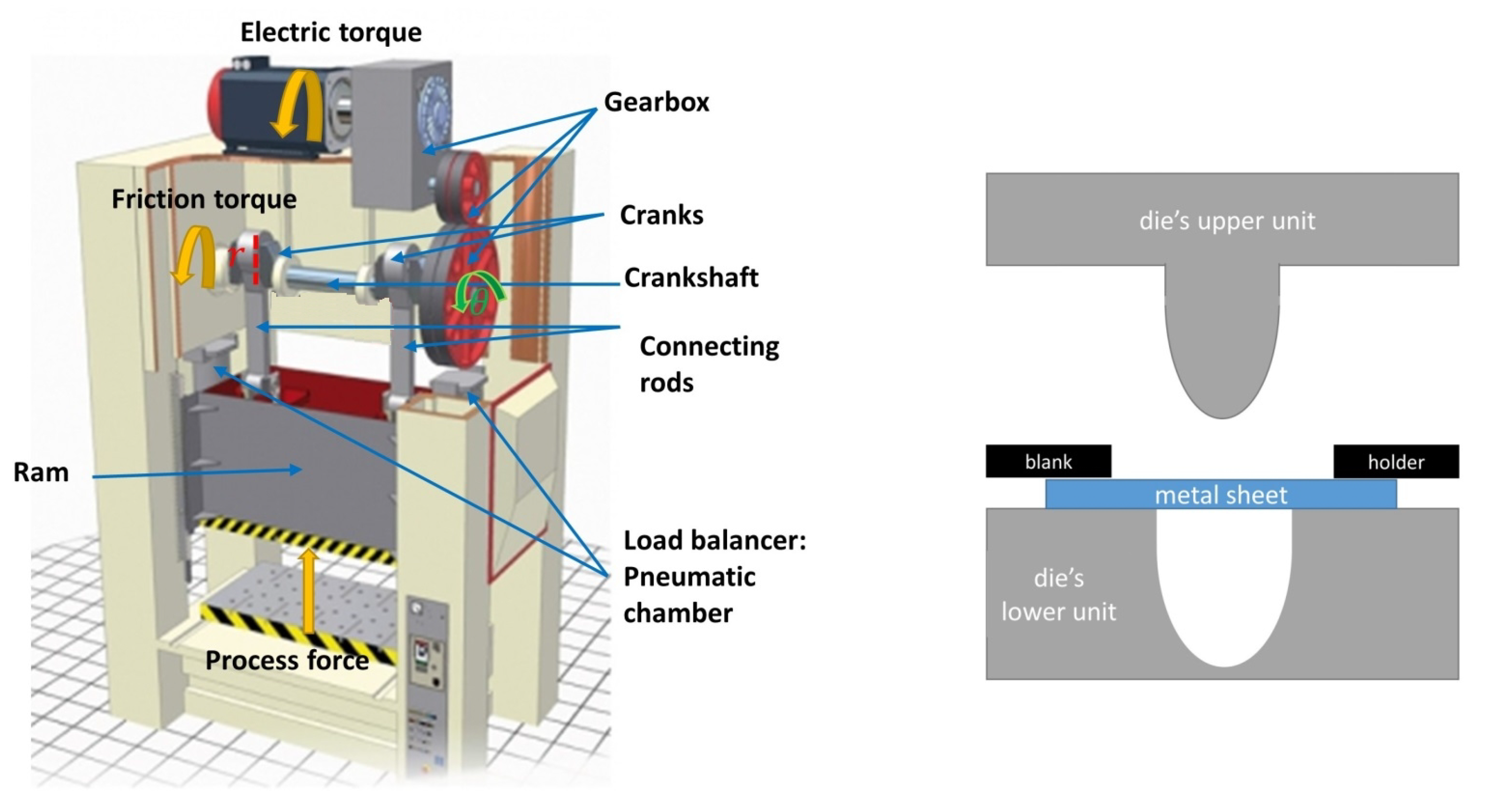
2.1. Process Data
2.2. Experimenting Procedure
2.3. Predictive Maintenance Techniques
3. Experimenting Results
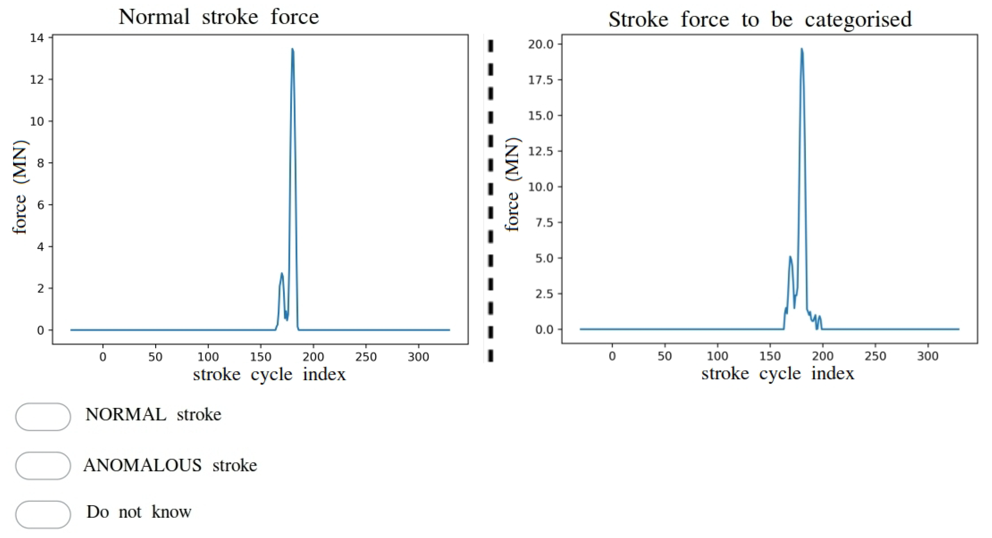
3.1. Anomaly Detection
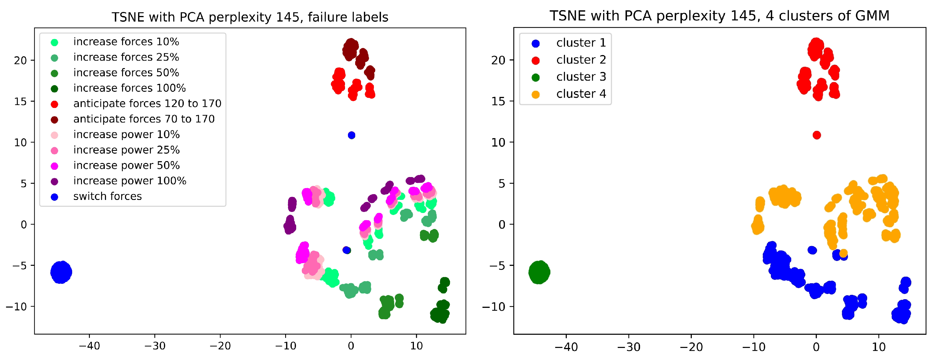
3.2. Diagnosis
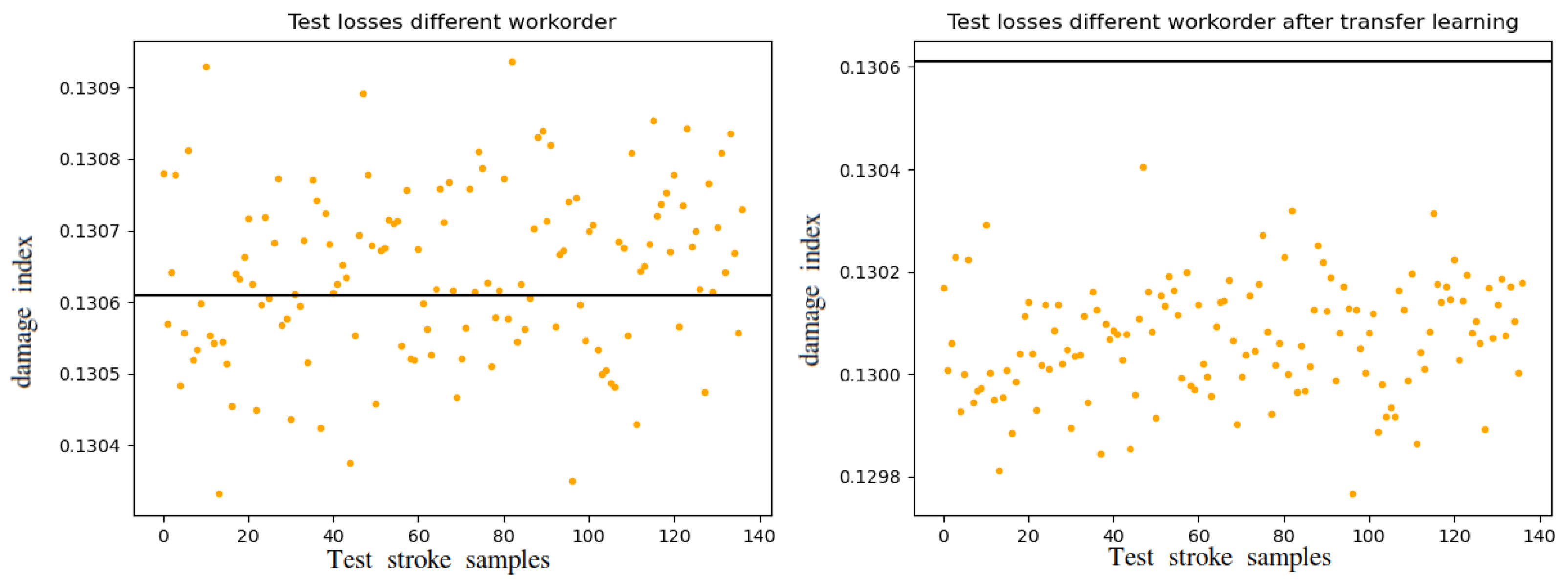
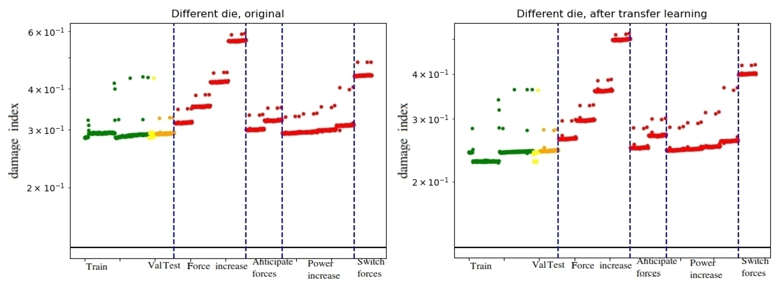
3.3. Adaptability
4. Discussion and Conclusions
Author Contributions
Funding
Institutional Review Board Statement
Informed Consent Statement
Data Availability Statement
Conflicts of Interest
Abbreviations
| 2D-CNN-AE | 2 dimensional convolutional-based autoencoder |
| ELM | Extreme learning machine |
| EOC | Environmental and operational conditions |
| GMM | Gaussian mixture models |
| OC-SVM | One-class support vector machines |
| OPTICS | Ordering points to identify the clustering structure |
| PCA | Principal component analysis |
| PdM | Predictive maintenance |
| SHAP | Shapley additive explanations |
| SOM | Self-organizing map |
| t-SNE | T-distributed stochastic neighbor embedding |
| XAI | Explainable artificial intelligence |
References
- Dhillon, B.S. Engineering Maintenance: A Modern Approach; CRC Press: Boca Raton, FL, USA, 2002; pp. 1–224. [Google Scholar]
- Wang, K.; Wang, Y. How AI Affects the Future Predictive Maintenance: A Primer of Deep Learning. In Advanced Manufacturing and Automation VII; Wang, K., Wang, Y., Strandhagen, J.O., Yu, T., Eds.; Springer: Singapore, 2018; pp. 1–9. [Google Scholar]
- UE Systems. Understanding the P-F Curve and Its Impact on Reliability Centered Maintenance. 2014. Available online: http://www.uesystems.com/news/understanding-the-p-f-curve-and-its-impact-on-reliability-centered-maintenance (accessed on 15 June 2021).
- Colemen, C.; Damodaran, S.; Chandramoulin, M.; Deuel, E. Making Maintenance Smarter; Deloitte University Press: New York, NY, USA, 2017. [Google Scholar]
- Lavi, Y. The Rewards and Challenges of Predictive Maintenance. InfoQ. 2018. Available online: https://www.infoq.com/articles/predictive-maintenance-industrial-iot (accessed on 28 May 2021).
- Jimenez-Cortadi, A.; Irigoien, I.; Boto, F.; Sierra, B.; Rodriguez, G. Predictive Maintenance on the Machining Process and Machine Tool. Appl. Sci. 2020, 10, 224. [Google Scholar] [CrossRef] [Green Version]
- Welz, Z.A. Integrating Disparate Nuclear Data Sources for Improved Predictive Maintenance Modeling: Maintenance-Based Prognostics for Long-Term Equipment Operation. Ph.D. Thesis, University of Tennessee, Knoxville, TN, USA, 2017. [Google Scholar]
- Venkatasubramanian, V.; Rengaswamy, R.; Yin, K.; Kavuri, S.N. A review of process fault detection and diagnosis: Part I: Quantitative model-based methods. Comput. Chem. Eng. 2003, 27, 293–311. [Google Scholar] [CrossRef]
- Serradilla, O.; Zugasti, E.; Zurutuza, U. Deep learning models for predictive maintenance: A survey, comparison, challenges and prospect. arXiv 2020, arXiv:2010.03207. [Google Scholar]
- Bampoula, X.; Siaterlis, G.; Nikolakis, N.; Alexopoulos, K. A Deep Learning Model for Predictive Maintenance in Cyber-Physical Production Systems Using LSTM Autoencoders. Sensors 2021, 21, 972. [Google Scholar] [CrossRef]
- Zhang, S.; Ye, F.; Wang, B.; Habetler, T.G. Semi-Supervised Bearing Fault Diagnosis and Classification using Variational Autoencoder-Based Deep Generative Models. IEEE Sens. J. 2020, 21, 6476–6486. [Google Scholar] [CrossRef]
- Bui, V.; Pham, T.L.; Nguyen, H.; Jang, Y.M. Data Augmentation Using Generative Adversarial Network for Automatic Machine Fault Detection Based on Vibration Signals. Appl. Sci. 2021, 11, 2166. [Google Scholar] [CrossRef]
- Kuo, R.; Li, C. Predicting Remaining Useful Life of Ball Bearing Using an Independent Recurrent Neural Network. In Proceedings of the 2020 2nd International Conference on Management Science and Industrial Engineering, Osaka, Japan, 7–9 April 2020; pp. 237–241. [Google Scholar]
- Yuan, J.; Wang, Y.; Wang, K. LSTM based prediction and time-temperature varying rate fusion for hydropower plant anomaly detection: A case study. In Advanced Manufacturing and Automation VIII. IWAMA 2018; Lecture Notes in Electrical Engineering; Springer: Singapore, 2019; Volume 484, pp. 86–94. [Google Scholar] [CrossRef]
- Schwartz, S.; Jimenez, J.J.M.; Salaün, M.; Vingerhoeds, R. A fault mode identification methodology based on self-organizing map. Neural Comput. Appl. 2020, 32, 13405–13423. [Google Scholar] [CrossRef]
- Talmoudi, S.; Kanada, T.; Hirata, Y. Tracking and visualizing signs of degradation for an early failure prediction of a rolling bearing. arXiv 2020, arXiv:2011.09086. [Google Scholar]
- Wen, L.; Gao, L.; Li, X. A new deep transfer learning based on sparse auto-encoder for fault diagnosis. IEEE Trans. Syst. Man Cybern. Syst. 2019, 49, 136–144. [Google Scholar] [CrossRef]
- Wen, T.; Keyes, R. Time Series Anomaly Detection Using Convolutional Neural Networks and Transfer Learning. arXiv 2019, arXiv:1905.13628. [Google Scholar]
- Martínez-Arellano, G.; Ratchev, S. Towards an active learning approach to tool condition monitoring with bayesian deep learning. In Proceedings of the ECMS 2019: 33rd International ECMS Conference on Modelling and Simulation, Caserta, Italy, 11–14 June 2019; Volume 33, pp. 223–229. [Google Scholar] [CrossRef]
- Zope, K.; Singh, K.; Nistala, S.; Basak, A.; Rathore, P.; Runkana, V. Anomaly detection and diagnosis in manufacturing systems: A comparative study of statistical, machine learning and deep learning techniques. Annu. Conf. PHM Soc. 2019, 11. [Google Scholar] [CrossRef]
- Brito, L.C.; Susto, G.A.; Brito, J.N.; Duarte, M.A. An explainable artificial intelligence approach for unsupervised fault detection and diagnosis in rotating machinery. Mech. Syst. Signal Process. 2022, 163, 108105. [Google Scholar]
- Lee, S.; Yu, H.; Yang, H.; Song, I.; Choi, J.; Yang, J.; Lim, G.; Kim, K.S.; Choi, B.; Kwon, J. A Study on Deep Learning Application of Vibration Data and Visualization of Defects for Predictive Maintenance of Gravity Acceleration Equipment. Appl. Sci. 2021, 11, 1564. [Google Scholar]
- Maschler, B.; Vietz, H.; Jazdi, N.; Weyrich, M. Continual learning of fault prediction for turbofan engines using deep learning with elastic weight consolidation. In Proceedings of the 25th IEEE International Conference on Emerging Technologies and Factory Automation (ETFA), Vienna, Austria, 8–11 September 2020; Volume 1, pp. 959–966. [Google Scholar]
- Maschler, B.; Kamm, S.; Weyrich, M. Deep industrial transfer learning at runtime for image recognition. at-Automatisierungstechnik 2021, 69, 211–220. [Google Scholar]
- Olaizola Alberdi, J. Soft Sensor-Based Servo Press Monitoring. Ph.D. Thesis, Mondragon Unibertsitatea, Goi Eskola Politeknikoa, Mondragon, Spain, 2020. [Google Scholar]
- Wold, S.; Esbensen, K.; Geladi, P. Principal component analysis. Chemom. Intell. Lab. Syst. 1987, 2, 37–52. [Google Scholar]
- Huang, G.B.; Zhu, Q.Y.; Siew, C.K. Extreme learning machine: Theory and applications. Neurocomputing 2006, 70, 489–501. [Google Scholar]
- Hejazi, M.; Singh, Y.P. One-class support vector machines approach to anomaly detection. Appl. Artif. Intell. 2013, 27, 351–366. [Google Scholar]
- Meire, M.; Karsmakers, P. Comparison of deep autoencoder architectures for real-time acoustic based anomaly detection in assets. In Proceedings of the 10th IEEE International Conference on Intelligent Data Acquisition and Advanced Computing Systems: Technology and Applications (IDAACS), Metz, France, 18–21 September 2019; Volume 2, pp. 786–790. [Google Scholar]
- Zugasti, E.; Iturbe, M.; Garitano, I.; Zurutuza, U. Null is not always empty: Monitoring the null space for field-level anomaly detection in industrial IoT environments. In Proceedings of the 2018 Global Internet of Things Summit (GIoTS), Bilbao, Spain, 4–7 June 2018; pp. 1–6. [Google Scholar]
- Van der Maaten, L.; Hinton, G. Visualizing data using t-SNE. J. Mach. Learn. Res. 2008, 9, 2579–2605. [Google Scholar]
- Ankerst, M.; Breunig, M.M.; Kriegel, H.P.; Sander, J. OPTICS: Ordering points to identify the clustering structure. ACM Sigmod Rec. 1999, 28, 49–60. [Google Scholar]
- Lindsay, B.G. Mixture models: Theory, geometry and applications. In NSF-CBMS Regional Conference Series in Probability and Statistics; Institute of Mathematical Statistics and the American Statistical Association: Boston, MA, USA, 1995; Volume 5, p. i-iii+v-ix+1-163. [Google Scholar]
- Kohonen, T. The self-organizing map. Proc. IEEE 1990, 78, 1464–1480. [Google Scholar]
- Lundberg, S.M.; Lee, S.I. A unified approach to interpreting model predictions. In Proceedings of the 31st International Conference on Neural Information Processing Systems, Long Beach, CA, USA, 4 December 2017; pp. 4765–4774. [Google Scholar]
- Lundberg, S. A Game Theoretic Approach to Explain the Output of Any Machine Learning Model. Github. 2021. Available online: https://github.com/slundberg/shap (accessed on 28 June 2021).
- Sundararajan, M.; Taly, A.; Yan, Q. Axiomatic attribution for deep networks. Proc. Mach. Learn. Res. 2017, 70, 3319–3328. [Google Scholar]
- Smilkov, D.; Thorat, N.; Kim, B.; Viégas, F.; Wattenberg, M. Smoothgrad: Removing noise by adding noise. arXiv 2017, arXiv:1706.03825. [Google Scholar]
- Tensorflow. TensorFlow 2.3 documentation. Available online: https://devdocs.io/tensorflow~2.3/ (accessed on 28 June 2021).
- Scik-it learn. Scik-it learn 0.23.2 documentation. Available online: https://scikit-learn.org/stable/whats_new/v0.23.html (accessed on 28 June 2021).
- Vettigli, G. Minisom documentation - Minimalistic and NumPy-based implementation of the Self Organizing Map. Available online: https://github.com/JustGlowing/minisom (accessed on 28 June 2021).


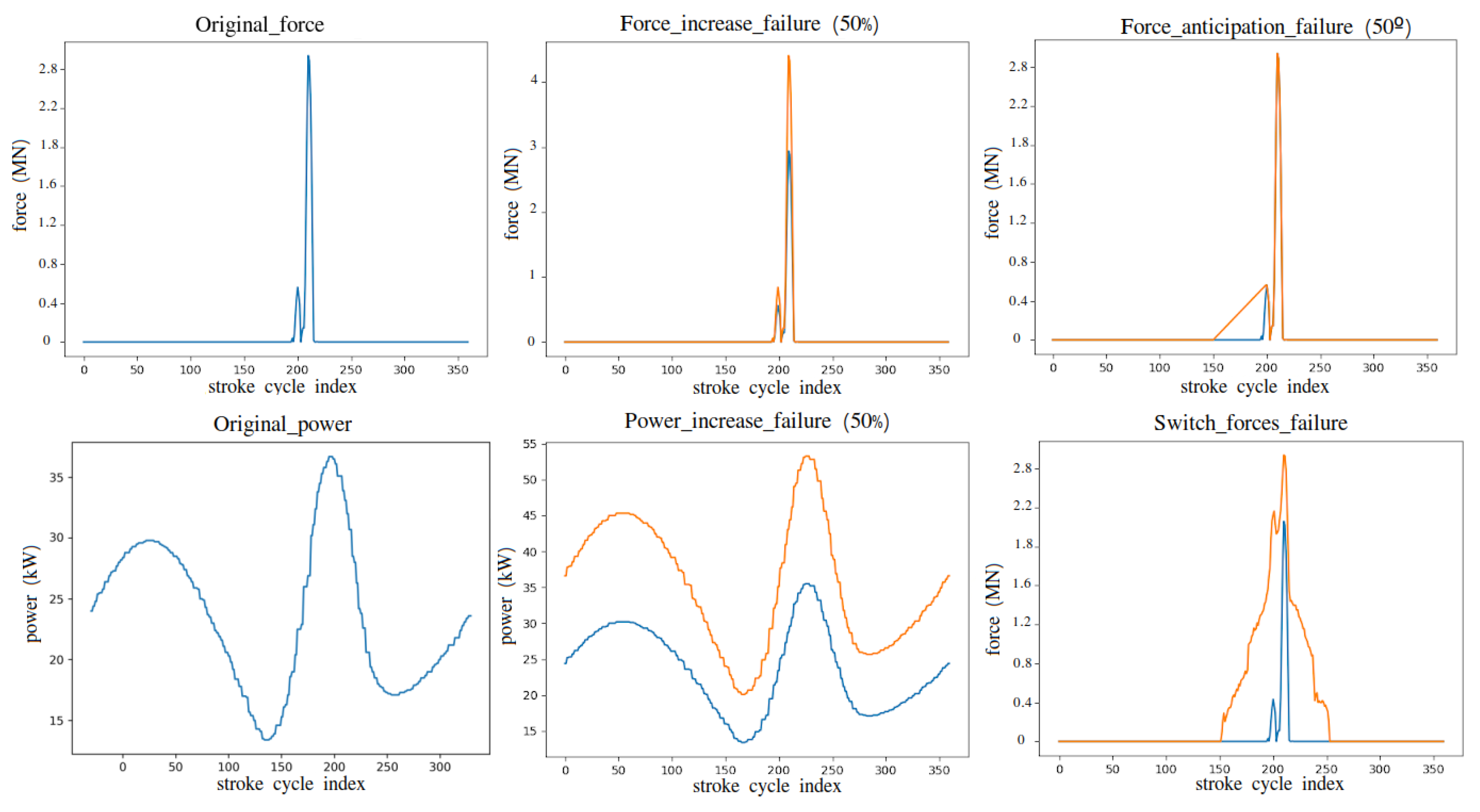
| Synthetic Failure | Signal Modification and Variations |
|---|---|
| Force increment, simulating harder input material | Increase forces on full signal 4 axis (+10%, +25%, +50% and +100%) |
| Die misadjustment, simulating press force anticipation | Anticipation of press force application (only 50 and 100) |
| Machine degradation, higher power consumption for same forces | Increase power consumption on full signal (+10%, +25%, +50% and +100%) |
| Unbalanced loads | Exchange press input and press output forces on full signal |
| Dataset | Data Type | Strokes in Train Set | Strokes in Validation Set | Strokes in Test Set for Each Type |
|---|---|---|---|---|
| For anomaly detection | Correct | 516 | 58 | 143 |
| For anomaly detection | Synthetic failure | 0 | 55 (5 for each type) | 143 |
| For transfer learning | Correct | 495 | 55 | 137 |
| For transfer learning | Synthetic failure | 0 | 55 (5 for each type) | 137 |
| Anomaly Detection Model | Training Parameters |
|---|---|
| PCA cycle | num. components = 90%; loss func. = RMSE |
| PCA trad. feats | num. components = 90%; loss func. = RMSE |
| ELM cycle | h_dim = 10; target = 1; loss func. = absolute diff. |
| ELM trad. feats | h_dim = 10; target = 1; loss func. = absolute diff. |
| OC-SVM cycle | kernel = rbf; kernel coef. = 1/n_features; nu = 1% |
| OC-SVM trad. feats | kernel = rbf; kernel coef. = 1/n_features; nu = 1% |
| Null-space | alpha = 5; beta = 5 |
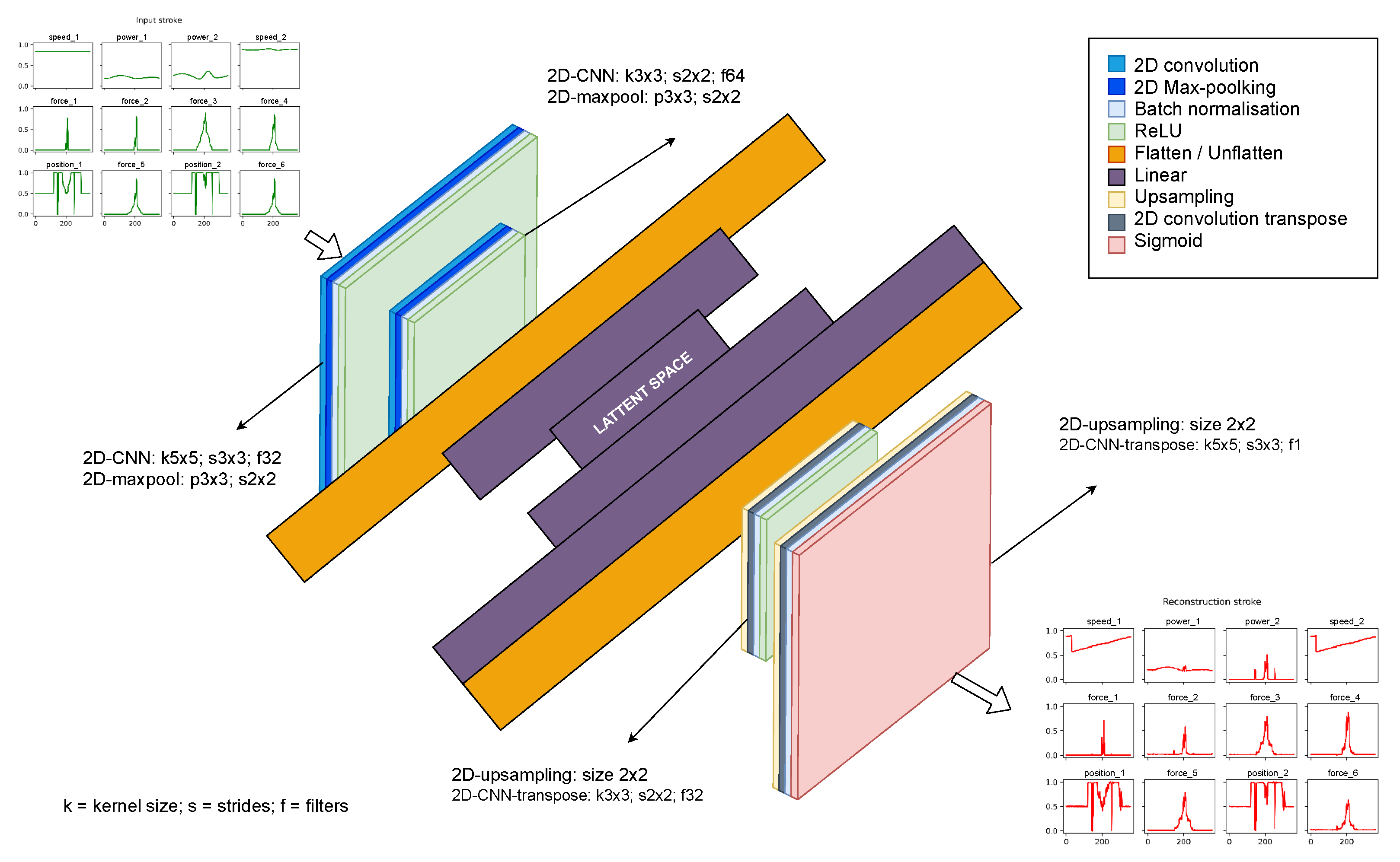
| 2D-CNN-AE | Input dim: batchxnum_cyclesx12x1 2 FE layers of 2D CNN&maxpool&relu&flatten&FFNN optimizer = adam (lr = 0.001, betas = (0.9, 0.999), eps = 1 ) early stopping, patience = 2 train loss = MSE; loss func = RMSE |
| Algorithm | (1) Force Increase | (2) Force Anticipation | (3) Power Increase | Switch Forces | |||||||
|---|---|---|---|---|---|---|---|---|---|---|---|
| 10% | 25% | 50% | 100% | 120–170 | 70–170 | 10% | 25% | 50% | 100% | ||
| PCA cycle | 0.27 | 0.74 | 0.97 | 0.97 | 0.09 | 0.93 | 0.10 | 0.16 | 0.65 | 0.97 | 0.97 |
| PCA feats | 0.67 | 0.67 | 0.67 | 0.67 | 0.67 | 0.67 | 0.02 | 0.09 | 0.62 | 0.67 | 0.67 |
| ELM cycle | 0.17 | 0.21 | 0.24 | 0.25 | 0.18 | 0.21 | 0.15 | 0.15 | 0.15 | 0.16 | 0.23 |
| ELM feats | 0.07 | 0.22 | 0.68 | 0.76 | 0.23 | 0.52 | 0.06 | 0.06 | 0.07 | 0.07 | 0.91 |
| OC-SVM cycle | 0.67 | 0.68 | 0.68 | 0.68 | 0.66 | 0.66 | 0.66 | 0.66 | 0.66 | 0.66 | 0.68 |
| OC-SVM feats | 0.41 | 0.67 | 0.67 | 0.67 | 0.47 | 0.67 | 0.08 | 0.06 | 0.04 | 0.02 | 0.67 |
| Null space | 0.82 | 1.00 | 1.00 | 1.00 | 1.00 | 1.00 | 0.47 | 1.00 | 1.00 | 1.00 | 1.00 |
| CNN-AE p90 | 0.91 | 0.91 | 0.91 | 0.91 | 0.91 | 0.91 | 0.91 | 0.91 | 0.91 | 0.91 | 0.91 |
| CNN-AE p95 | 0.99 | 0.99 | 0.99 | 0.99 | 0.99 | 0.99 | 0.99 | 0.99 | 0.99 | 0.99 | 0.99 |
| Number Clusters | (3) Power Increase | (2) Force Anticipation | (1) Force Increase | (4) Switch Forces | ||||
|---|---|---|---|---|---|---|---|---|
| prec | rec | prec | rec | prec | rec | prec | rec | |
| outliers | 0.41 | 0.74 | 0.20 | 0.72 | 0.40 | 0.72 | 0.00 | 0.00 |
| 1 | 0.75 | 0.26 | 0.00 | 0.00 | 0.25 | 0.09 | 0.00 | 0.00 |
| 2 | 0.00 | 0.00 | 1.00 | 0.28 | 0.00 | 0.00 | 0.00 | 0.00 |
| 3 | 0.00 | 0.00 | 0.00 | 0.00 | 1.00 | 0.19 | 0.00 | 0.00 |
| 4 | 0.00 | 0.00 | 0.00 | 0.00 | 0.00 | 0.00 | 1.00 | 1.00 |
Publisher’s Note: MDPI stays neutral with regard to jurisdictional claims in published maps and institutional affiliations. |
© 2021 by the authors. Licensee MDPI, Basel, Switzerland. This article is an open access article distributed under the terms and conditions of the Creative Commons Attribution (CC BY) license (https://creativecommons.org/licenses/by/4.0/).
Share and Cite
Serradilla, O.; Zugasti, E.; Ramirez de Okariz, J.; Rodriguez, J.; Zurutuza, U. Adaptable and Explainable Predictive Maintenance: Semi-Supervised Deep Learning for Anomaly Detection and Diagnosis in Press Machine Data. Appl. Sci. 2021, 11, 7376. https://doi.org/10.3390/app11167376
Serradilla O, Zugasti E, Ramirez de Okariz J, Rodriguez J, Zurutuza U. Adaptable and Explainable Predictive Maintenance: Semi-Supervised Deep Learning for Anomaly Detection and Diagnosis in Press Machine Data. Applied Sciences. 2021; 11(16):7376. https://doi.org/10.3390/app11167376
Chicago/Turabian StyleSerradilla, Oscar, Ekhi Zugasti, Julian Ramirez de Okariz, Jon Rodriguez, and Urko Zurutuza. 2021. "Adaptable and Explainable Predictive Maintenance: Semi-Supervised Deep Learning for Anomaly Detection and Diagnosis in Press Machine Data" Applied Sciences 11, no. 16: 7376. https://doi.org/10.3390/app11167376
APA StyleSerradilla, O., Zugasti, E., Ramirez de Okariz, J., Rodriguez, J., & Zurutuza, U. (2021). Adaptable and Explainable Predictive Maintenance: Semi-Supervised Deep Learning for Anomaly Detection and Diagnosis in Press Machine Data. Applied Sciences, 11(16), 7376. https://doi.org/10.3390/app11167376