Abstract
The paper presents possible approaches for reducing the volume of data generated by simulation optimisation performed with a digital twin created in accordance with the Industry 4.0 concept. The methodology is validated using an application developed for controlling the execution of parallel simulation experiments (using client–server architecture) with the digital twin. The paper describes various pseudo-gradient, stochastic, and metaheuristic methods used for finding the global optimum without performing a complete pruning of the search space. The remote simulation optimisers reduce the volume of generated data by hashing the data. The data are sent to a remote database of simulation experiments for the digital twin for use by other simulation optimisers.
1. Introduction
The increasing use of digital twins (DTs) is one of the most important trends in the Industry 4.0 concept and industrial engineering [1], and some authors directly refer to the Industry 4.0 era as the era of DT [2]. The concept of Industry 4.0 extends the possibilities and use of DTs for, e.g., decision support and production planning [3], solving unexpected situations/problems or predicting such situations [4], as well as training and knowledge transfer of leadership, management, and executives [5,6].
In addition to DTs, the use of cyber–physical systems (CPSs) is increasingly mentioned in connection with the Industry 4.0 concept. A CPS is a system consisting of physical entities controlled by computer algorithms that allow these entities to function completely independently, including autonomous decision making, i.e., they can control a given technological unit or be an independent member of complex production units. CPSs are often built on artificial intelligence and machine learning [6], using simulations [7] for decision making and other areas of computer science that are being developed within the Industry 4.0 concept.
The goal of our research is to test and modify different optimisation methods (and also their settings) suitable for discrete simulation optimisation in accordance with the Industry 4.0 concept. A large number of data are generated during the simulation experimentation with a DT. This paper describes a proposed methodology for reducing the volume of generated data in a simulation optimisation performed with a DT. The methodology attempts to avoid the problem of generating big data rather than trying to extract information from the large volume of generated data (often representing inappropriate solutions). We were inspired by different techniques used in the field of big data problems. We had to solve many problems during the simulation experimentation, e.g., reduction of the generated data while maintaining the amount of necessary information without the loss of accuracy needed for the simulation optimisation; ensuring a high search speed of these data; using the parallelisation of the DT simulation experimentation; reducing the redundant data; preventing possible data loss during the simulation experimentation with DT, etc.
We used various optimisation methods (stochastic, metaheuristic–population or neighbourhood-based algorithms), which are used in the optimisation of processes of the DT. The proposed methodology was validated on several simulation studies (both theoretical and practical). We selected the case of a DT of automated guided vehicles (AGVs) conveying different types of parts to assembly lines from warehouses to describe the methodology proposed in this paper.
The effectiveness of different optimisation methods in finding a suitable solution is not the same. It differs especially in the case of different objective function landscapes (the objective function of the DT is the goal we want to achieve). The paper describes the evaluation of simulation experiments using different optimisation methods. These evaluations are analysed from different perspectives (quality of found solution, the speed of finding the solution, etc.). The effectiveness of the optimisation method also depends on both the principle of the method and the settings of its parameters. We tested different settings to compare the effectiveness of the optimisation methods. If the optimisation method is set up well, it does not need to perform many simulation experiments, and thus, the number of generated data is reduced.
2. Literature Background
Both CPS and DT are aimed at achieving the cyber–physical integration needed for smart manufacturing, but each approach emphasises something different. While CPS focuses on sensors and actuators, DT focuses on data and models [8]. The relationship between CPS and DT can be described in that CPS uses DT, and existing DT is a prerequisite for CPS [9]. Cyber–physical systems produce a large number of data; thus, big data analytics is used for them, e.g., for predictability, planning, and decision making [10]. The relationship between CPS and DT can be seen in Figure 1.
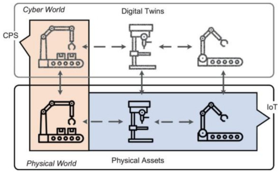
Figure 1.
Relationship between CPS, DT, and IoT [11].
Big data analytics is a core component of data-based smart manufacturing and Industry 4.0 initiatives [12]. The term big data originated in the early 1990s and refers to data that are large in volume, variously heterogeneous (mainly in terms of structure), and with uncertain credibility due to their possible inconsistency or, for example, incompleteness, and with fast processing often required. Thus, the basic characteristics of big data are the three Vs—‘Volume’, ‘Veracity’, and ‘Variety’ [13]. Over time, the three Vs have been extended to five Vs by the addition of ‘Value,’ the value of the data (often relative to a point in time), and ‘Velocity,’ the rapid increase in the volume of the data [14]. Big data processing often encounters the limitations of traditional databases, software technologies, and established processing methodologies [15].
Generally, there are two main functional components—system infrastructures and data analytics—used to address the issue of big data in CPS in Industry 4.0. System infrastructure provides real-time communication between devices and cyber devices, while data analytics focuses on improving product personalisation and efficiency of resource utilisation [16].
As the processing of large volumes of data exceeds the capabilities of commonly used computers, supercomputers or clusters are used. Since supercomputers are very expensive, distributed computing systems (clusters) are more available, more cost effective, and widely used in industry [17].
Big data mostly generates CPS, ERP systems, etc. within the Industry 4.0 concept. These big data are analysed, cleansed, and mined, and the obtained data are then used as input for simulations, based on the results of which the parameters and properties of the CPS are then adjusted, or the simulations are used as a semantic validator, as shown in Figure 2.
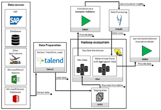
Figure 2.
Steps required to provide semantically valid data to the simulation model [18].
The approach presented in this paper is inspired by this standard approach. The difference, however, is that the simulation models generate large volumes of data that are reduced using a hashing algorithm. Network architecture is used to communicate over a shared database to reduce unnecessary computations on the simulation model if a given variant has already been realised by a simulation optimiser. Moreover, it is possible to set up different scenarios with data storage in the memory of each simulation optimiser.
2.1. Simulation Optimisation
The data used for the simulation optimisation to mimic the possible scenarios of the process are obtained from the enterprise information system, e.g., enterprise resource planning (ERP). These data are very good for strategic or tactical planning (not so often used for operative planning) or control.
Using the internet of things (IoT), it is possible to read or download the data from the different objects in the company, e.g., the production lines, AGVs, etc. These data are especially suitable for operative planning or control. The current data processing is beyond the computing ability of traditional computational models due to the immense volume of constantly or exponentially generated data from the objects in the company.
Researchers in data analytics use and design new efficient algorithms to handle massive data analytics problems, e.g., population-based algorithms including swarm intelligence and evolutionary algorithms—see Figure 3. These methods are used for extracting useful information from a big volume of raw data.
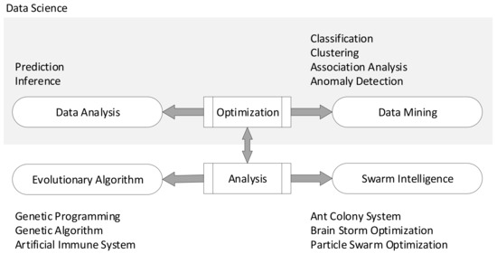
Figure 3.
Relationship between data science with evolutionary algorithm and swarm intelligence [19].
Some of our department’s projects are also focused on the simulation of processes in industrial companies. We create DTs (discrete event simulation models) which represent real physical processes in different parts of a company (mainly production lines, warehouses, etc.). The main problem of these simulation studies (mainly focusing on the optimisation of the modelled processes) is the big search space (many possible solutions to the modelled problem). The volume of data generated by the optimisation processes is also affected by the number of the simulation model input parameters. The search space is usually boundary constrained as follows:
where
- denotes the search space—the domain of the input parameters of the discrete event simulation model;
- denotes the index of the -th decision variable (simulation model input parameter) of the simulation model;
- denotes the dimension of the search space;
- denotes the lower bound of the interval of the -th decision variable;
- denotes the upper bound of the interval of the -th decision variable.
Many of the modelled problems are NP-hard problems in which we often cannot evaluate all the possible solution candidates,
where
- denotes a possible solution candidate;
- denotes the value of the -th decision variable.
The basic problem of the simulation optimisation is to find the optimum of the objective function representing the aim of the simulation optimisation as follows:
where
- denotes the global minimum of the objective function ;
- denotes the objective function value of the solution candidate. The objective function represents the goal of the simulation study. Each solution candidate (possible solution of the modelled problem representing the vector of the values for each decision variable in search space) is evaluated by the objective function value—the range includes real numbers . The objective function maximisation can be converted to function minimisation.
Testing all possible solutions to a problem is a very inefficient way (and mostly impossible) of finding a suitable solution candidate or the global optimum. This is the reason why various global optimisation methods (especially the metaheuristic methods) use different strategies to find a suitable solution candidate and to reduce this vast space (some algorithms keep suitable tested solutions and provide a set of optima instead of a single solution). Many of the optimisation algorithms (especially population-based algorithms—naturally inspired or evolutionary algorithms) generate, instead of a small number of solution candidates, the whole population containing a big number of these solution candidates which are iteratively refined as follows:
where
- denotes the -th generated solution candidate;
- denotes the list—population—of generated solution candidates;
- denotes the length of the list —population size.
These data must be stored to keep the information about the quality of the tested possible solution in the optimisation process. The question is how to keep all this information which can be used for subsequent optimisations? We propose a methodology which helps to reduce the volume of the data generated from the simulation optimisation.
2.2. Optimisation Methods
Simulation optimisation techniques are mostly used for the following:
- Discrete event simulation;
- Systems of stochastic nonlinear and/or differential equations [20].
There are many algorithms for simulation optimisation, and their use depends on the specific application. In their paper, the authors Su et al. [21] describe the following as the basic algorithms for simulation optimisation:
- Ranking and selection;
- Black-box search methods that directly work with the simulation estimates of objective values;
- Meta-model-based methods;
- Gradient-based methods;
- Sample path optimisation;
- Stochastic constraints and multi-objective simulation optimisation.
Considering the applicability of simulation optimisation in many industries and aspects of human activities and its generality, there are many studies using simulation optimisation in areas of industrial product development such as maintenance systems [22], industrial production lines [23], new product development [24,25], etc.
Among the random optimum search methods, techniques such as simulated annealing [26], genetic algorithms [27], stochastic ruler methods [28], ant colony optimisation [29], tabu search [30], etc. are used for the optimisation. For most of these algorithms, there is evidence of global convergence, i.e., convergence to a global solution or local convergence [31].
The paper [32] analyses a significant sample size (663 research papers) to provide insights about the past and present practices in discrete simulation-based optimisation (DSBO) applied to industrial engineering. DSBO is a set of tools and methods commonly used to help researchers and practitioners, for analysis and decision making, for investment and resource allocation in new or already existing systems. Many articles published in this area refer to the solution of a specific problem using one or more methods. The following table presents the state-of-the-art techniques applied to DSBO projects on IE problems (NP-hard), showing the past and present practices and bringing up possibilities for the future of DSBO on IE—see Table 1.

Table 1.
DSBO methods used [32].
Many authors focus on the optimisation of a specific problem with one optimisation method or a modified derived optimisation method. Unfortunately, they do not address the applicability of multiple optimisation methods to multiple problems and the comparison of the effectiveness of these methods using the different evaluation criteria (not just using the average, mean, or standard deviation). We tested different optimisation methods (stochastic, metaheuristic–population, or neighbourhood-based algorithms) solving different problems in industrial engineering (logistics, production planning, etc.) using discrete-event simulation models. We were also interested in the evaluation of optimisation experiments with different settings of the optimisation methods (big volume of data) from different perspectives [33]. We proposed a methodology that can be applied to the optimisation of several industrial engineering problems represented by a discrete-event simulation model.
The proposed methodology for parallel simulation optimisation uses the server’s simulation optimiser (architecture client–server) using stochastic, neighbourhood-, and population-based optimisation methods. Using the right method can significantly reduce the search space as it reduces the data generated in the optimisation process.
2.2.1. Random Search
A population of new individuals (solution candidates) is generated in the search space with uniform distribution using the Monte Carlo method. This method is suitable where the user has no information about the objective function type. The user can set the possibility of generating the same possible solution by this optimisation method. This option is useful when the search space of the simulation model is quite small.
2.2.2. Downhill Simplex
This optimisation method uses the idea of the Nelder–Mead downhill simplex algorithm [34]. This heuristic method uses a set of n + 1 linearly independent points, i.e., possible solutions (individuals) in the search space—simplex,
where
- denotes the simplex;
- denotes the first solution candidate;
- denotes the dimension of the search space;
- denotes the search space—the domain of the input parameters of the discrete event simulation model—solution candidates.
If we evaluate points with the objective function (objective function minimisation), we have
where
- denotes the worst solution candidate of the simplex;
- denotes the best solution candidate;
- denotes the objective function value of the solution candidate;
- denotes the simplex centroid—centre of gravity (calculated from the solution candidate apart from the best solution candidate).
The method uses the following four basic phases of generating a solution candidate–see Figure 4 [35]:
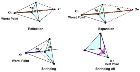
Figure 4.
The principle of the Nelder–Mead downhill simplex method [35].
- Reflection—mirroring the worst solution candidate;
- Expansion—searching for a better solution in the reflection direction;
- Contraction—testing the solution candidate between reflection and simplex centroid
- Reduction—shrinkage towards the best solution candidate of the simplex.
If we want to use this optimisation method for a discrete-event simulation optimisation, the problem is rounding of the point coordinates in the search space (the point coordinates are the vector of the values of the simulation model input parameters) to the nearest feasible coordinates in the search space. This leads to deviation from the original direction in our case if the step of the axis, the decision variable, in the search space is large. A detailed description of this implemented optimisation method is described in [36,37].
2.2.3. Stochastic Hill Climbing
Possible solutions—individuals—are generated (populated) in the neighbourhood of the best solution candidate from the previous population. Generating new possible solutions is performed by mutation. This method is part of the family of local search methods. The problem of this method is getting stuck in the local extreme, namely, in the case of multimodal function—premature convergence. This problem can be solved by random restarts of this method [36].
The next algorithm shows the principle of stochastic hill climbing—see Algorithm 1. The function creates the initial population of solutions candidates. Function sorts the population of solutions candidates according to their quality. The quality includes the objective function value of the solutions candidate. The function adds the item in the list, i.e., adds the solution candidate to the population.
| Algorithm 1: Stochastic Hill-Climbing Algorithm Pseudocode | |
| 1 | begin |
| 2 | ; //initial population |
| 3 | ; //sort in ascending order according to |
| 4 | ; //the best solutions candidate in |
| 5 | ; |
| 6 | while not do begin //termination criterion |
| 7 | ; //delete |
| 8 | for to do begin |
| 9 | ; (*mutation of best solutions candidate in -uniform distribution*) |
| 10 | for to do //for each gen of |
| 11 | //perturbation |
| 12 | ; //add new solutions candidate to |
| 13 | end; |
| 14 | ; |
| 15 | ; |
| 16 | if then //better solutions candidate was found |
| 17 | ; |
| 18 | end; |
| 19 | result ; |
| 20 | end; |
We use the perturbation repair algorithm for the correction of the point coordinates outside of the search space (we can call it the ‘repair’ of the defective gene). This algorithm mirrors the possible solution coordinates of the solution candidate back to the search space—see Algorithm 2.
| Algorithm 2: Perturbation Pseudocode | |
| 1 | begin |
| 2 | ; |
| 3 | if then |
| 4 | ; |
| 5 | while do begin |
| 6 | if then |
| 7 | //mirror the solutions candidate coordinate back to search space |
| 8 | else if then |
| 9 | ; |
| 10 | ; (* round or truncate the coordinate of the solutions candidate in the search space to the nearest neighbour *) |
| 11 | end; |
| 12 | result ; |
| 13 | end; |
2.2.4. Stochastic Local Search
The difference between the local search algorithm and the hill-climbing algorithm is that we accept the new solution candidate if this solution candidate is better than the best-found solution candidate from the start of the algorithm—see Algorithm 3.
| Algorithm 3: Stochastic Local Search Pseudocode | |
| 1 | begin |
| 2 | ; //generating individual |
| 3 | while not do begin //termination criterion |
| 4 | ; (*mutation of the best-found individual *) |
| 5 | for to do //for each gen of the individual |
| 6 | //perturbation |
| 7 | if then //better solution candidate was found |
| 8 | ; |
| 9 | end; |
| 10 | result ; |
| 11 | end; |
2.2.5. Stochastic Tabu Search
The method of searching with tabus, or simply ‘tabu search’ or ‘tabu method’, was formalised in 1986 by Fred W. Glover. Its principal characteristic is based on the use of mechanisms inspired by human memory. The tabu method takes a path opposite to that of simulated annealing, which does not utilise memory at all and thus is unable to learn lessons from the past [38,39].
A newly generated solution candidate is an element of the tabu list during the optimisation process. This solution candidate cannot be visited again if the aspiration criterion is not satisfied (this feature prevents the method from becoming stuck at a local optimum). The method uses the FIFO method of removing the solution candidate from the tabu list. The user can set whether the new solution candidate is generated using mutation of the best solution candidate from the previous population or the mutation of the best-found solution candidate, that is, the best individual found from the start of the optimisation process [36].
The next algorithm shows the principle of the stochastic tabu search method—see Algorithm 4. The algorithm uses the function for appending the list of solution candidates to the tabu list—joining two populations together. The next function searches an unsorted list and provides the information if the item is in the list—the population contains a solution candidate. The function deletes the item from the list, meaning that it deletes the solution candidate from the population.
| Algorithm 4: Stochastic Tabu Search Pseudocode | |
| 1 | begin |
| 2 | ; //initial population |
| 3 | ; //sort population |
| 4 | ; //best solution candidate from |
| 5 | ; |
| 6 | ; //empty Tabu List |
| 7 | ; |
| 8 | while not do begin //termination criterion |
| 9 | ; //empty |
| 10 | for to do begin |
| 11 | repeat |
| 12 | ; |
| 13 | for to do //for each gen of solution candidate |
| 14 | //perturbation |
| 15 | ; //add to |
| 16 | until or ; //solution candidate is not element of or meet the aspiration criterion |
| 17 | if then |
| 18 | ; |
| 19 | ; |
| 20 | ; |
| 21 | end; |
| 22 | ; |
| 23 | ; |
| 24 | if then //better solution candidate was found |
| 25 | ; |
| 26 | end; |
| 27 | result ; |
| 28 | end; |
2.2.6. Stochastic Simulated Annealing
Simulated annealing (SA) uses a principle used in metallurgy and material science, namely, the heat treatment of a material to alter the properties of the material. Metal crystals have small defects and dislocations, which weaken the structure. The structure of the material can be improved by heating and cooling the material [36].
SA is one of the most flexible techniques available for solving hard combinatorial problems. The main advantage of SA is that it can be applied to large problems regardless of the conditions of differentiability, continuity, and convexity that are normally required in conventional optimisation methods [40].
The idea of stochastic simulated annealing uses a possible solution generated in the neighbourhood of the solution candidate from the previous iteration. The cooling schedule (the control strategy) is characterised by the initial temperature; the final temperature; the number of transitions and the temperature rate of change [40,41].
We modified the SA algorithm presented in [36], which uses the metropolis procedure where the non-negative parameter of temperature reduction, the minimum temperature, the acceptance probability, and the energetic difference between the current and the new geometry are used. A detailed description of our implemented method of simulated annealing is described in [37].
2.2.7. Differential Evolution
Methods such as differential evolution, self-organising migrating algorithm (SOMA), evolutionary strategies, and genetic algorithm are evolutionary computation methods. These methods use the term ‘individual’ instead of ‘solution candidate’, but the meaning is the same.
The differential evolution technique belongs to the class of evolutionary algorithms. In fact, it is founded on the principles of mutation, crossover, and selection. However, it was originally conceived [42] for continuous problems and it uses a weighted difference between two randomly selected individuals as the source of random variations. The method is very effective and has recently become increasingly popular. Thus, the core of the method is based on a particular manner of creating new individuals. A new individual is created by adding the weighted difference between the two individuals with a third; if the resulting vector is better than a predetermined individual, the new vector replaces it. Thus, the algorithm extracts information about direction and distance to produce its random component [39,43].
The algorithm of differential evolution uses selection which is carried out between the parent (solution candidate) and its offspring in the population. The better individual of the two compared individuals is then assigned to a population that completely replaces the parent population. The question is how to create an individual that will subsequently be crossed with the parent. There are several ways of creating such an individual. The first method generates an individual (mutation) using three different individuals randomly selected from the parent population. These individuals must further satisfy the condition that they must be different from the individual just selected from the parent population.
The second basic method of generating a new individual by mutation is using four randomly different individuals in a population and the best individual in the population that is different from these individuals. Further, the best individual and the four selected individuals must be different from the individual just selected from the parent population.
A detailed description of our implemented method of differential evolution is described in [37].
2.2.8. Self-Organising Migrating Algorithm (SOMA)
SOMA is based on the self-organising behaviour of groups of individuals in a ‘social environment’. It can also be classified as an evolutionary algorithm, even though no new generations of individuals are created during the search. Only the positions of the individuals in the search space are changed during a generation, called a ‘migration loop’. Individuals are generated at random according to what is called the ‘specimen of the individual’ principle. The specimen is in a vector, which comprises an exact definition of all these parameters that together led to the creation of such individuals, including the appropriate constraints of the given parameters. SOMA is not based on the philosophy of evolution (two parents create one new individual—the offspring) but on the behaviour of a social group of individuals [44,45].
The SOMA optimisation method is derived from differential evolution. There are different modifications of differential evolution, e. g., [43,46,47].
The mass parameter denotes how far the currently selected individual stops from the leader individual (if the , then the currently selected individual stops at the position of the leader; if the , then the currently selected individual stops behind the position of the leader, which equals the distance of the initial position of the currently selected individual and the position of the leader). If the , then the currently selected individual stops in front of the leader which leads to degradation of the migration process (the algorithm finds only local extremes). Hence, it is recommended to use . It is also recommended to use the following lower and upper boundaries of the parameter .
The step parameter denotes the resolution of mapping the path of the currently selected individual. It is possible to use a larger value for this parameter to accelerate the searching of the algorithm if the objective function is unimodal (convex function, few local extremes, etc.). If the objective function landscape is not known, it is recommended to use a low value for this parameter. The search space will be scanned in more detail, and this increases the probability of finding the global extreme. It is also important to set the Step parameter in a way that the distance of the currently selected individual, and the leader is not an integer multiple of this parameter (the diversity of the population is reduced because everyone could be pulled to the leader and the process of searching for the optimum could stop at a local extreme). Hence, it is recommended to use instead of . The setting of, e.g., also rapidly increases the effectiveness of the SOMA strategy, all to all.
PRT parameter denotes the perturbation. The perturbation vector contains the information on whether the movement of the currently selected individual toward the leader should be performed. It is one of the most important parameters of this optimisation method, and it is very sensitive. It is recommended to use . If the value of this parameter increases, then the convergence of the SOMA algorithm to local extremes also rapidly increases. It is possible to set this parameter to if many individuals are generated and if in the dimension of the search space the objective function is low. If , then the stochastic part of the behaviour of SOMA is cancelled, and the algorithm behaves according to deterministic rules (local optimisation of the multimodal objective function).
The NP parameter denotes how many individuals are generated in a population. If this parameter is set to , the SOMA algorithm behaves similar to a traditional deterministic method.
Generally, if n (where n denotes the dimension of the search space) is a higher number, then this parameter can be set to . If the objective function landscape is simple, we can use a lower number of generated individuals. If the objective function is complicated, we can set this parameter . It is recommended to use .
This parameter is equivalent to the ‘generation’ parameter used in other evolutionary algorithms. This parameter denotes the number of population regenerations [44,48].
2.2.9. Evolution Strategy
Evolution strategies (ES) introduced by Rechenberg [49] are a heuristic optimisation technique based on the ideas of adaptation and evolution, a special form of the evolutionary algorithm [50,51].
Evolution Strategies have the following features:
- They usually use vectors of real numbers as solution candidates. In other words, both the search and the problem space are fixed-length strings of floating-point numbers, such as the real-encoded genetic algorithms;
- Mutation and selection are the primary operators and recombination is less common;
- Mutation most often changes the solution candidate gene to a number drawn from a normal distribution;
- The values of standard deviations are governed by self-adaptation [52,53,54] such as covariance matrix adaptation [55,56,57,58,59];
- In all other aspects, they perform exactly as basic evolutionary algorithms.
The algorithm can use different population strategies: (1 + 1)—the population only consists of a single individual, which is reproduced. From the elder and the offspring, the better individual will survive and form the next population; (μ + 1)—the population contains μ individuals from which one is drawn randomly. This individual is reproduced from the joint set of its offspring and the current population, the least fit individual is removed; (μ + λ)—using the reproduction operations, from μ parent individuals λ ≥ μ offspring are created. From the joint set of offspring and parents, only the μ fittest ones are kept; (μ, λ)—in (μ, λ) evolution strategies, introduced by Schwefel [60], again λ ≥ μ children are created from μ parents. The parents are subsequently deleted, and from the λ offspring individuals, only the μ fittest are retained [60,61];
(μ/ρ, λ)—evolution strategies named (μ/ρ, λ) are basically (μ, λ) strategies. The additional parameter ρ is added, denoting the number of parent individuals of one offspring. As already mentioned, we normally only use mutation (ρ = 1). If recombination is also used as in other evolutionary algorithms, ρ = 2 holds. A special case of (μ/ρ, λ) algorithms is the (μ/μ, λ) evolution strategy [1] (μ/ρ + λ)—analogously to (μ/ρ, λ)—evolution strategies, the (μ/ρ + λ)—evolution strategies are (μ, λ) approaches where ρ denotes the number of parents of an offspring individual; (μ′,λ′ (μ,λ)γ)—Geyer et al. [2,3,4] have developed nested evolution strategies [62], where λ′ offspring are created and isolated for γ generations from a population of the size μ′. In each of the γ generations, λ children are created from which the fittest μ are passed on to the next generation. After γ generations, the best individuals from each of the γ isolated solution candidates are propagated back to the top-level population, i.e., selected. Then, the cycle starts again with λ′ new child individuals. This nested evolution strategy can be more efficient than the other approaches when applied to complex multimodal fitness environments [36,63,64].
Our implemented algorithm uses steady-state evolution where the number of successes (the offspring is better than the parent) is monitored by the relative frequency of success. An offspring is generated by the mutation of its parent using a normal distribution with defined deviations for each gene (axes of the search space—gen in genotype) which is affected by Rechenberg 1/5th-rule. A detailed description of our implemented method of evolution strategy is described in [65].
2.2.10. Particle Swarm Optimisation (PSO)
The PSO algorithm is a stochastic population-based optimisation method proposed by Eberhart and Kennedy in 1995 [66].
Comparisons with other evolutionary approaches have been provided by Eberhart and Shi [5].
PSO is a computational method which optimises a problem iteratively, trying to improve a particle (representing the solution candidate). PSO is a form of swarm intelligence simulating the behaviour of a biological social system, i.e., a flock of birds or a school of fish [67].
When a swarm looks for food, its particles will spread in the environment and move around independently. Each individual particle has a degree of freedom or randomness in its movements, which enables it to find food accumulations. Therefore, eventually, one of them will find something digestible and, being social, announces this to its neighbours. These can then approach the source of food [36].
The positions and velocities of all particles are randomly initialised in the initial phase of the PSO algorithm. The velocity of a particle is updated and then its position in each step. Therefore, each particle has a memory holding its best position. To realise the social component, the particle furthermore knows a set of topological neighbours. This set could be defined to contain adjacent particles within a specific perimeter, i.e., all individuals that are no further away from the position of the particle than a given distance according to a certain distance (Euclidian distance) [36].
Particle swarm optimisation has been discussed [68,69,70,71], improved [72,73,74,75], and refined by many researchers.
A detailed description of our implemented method of particle swarm optimisation is described in [76].
3. Digital Twin
The DT is the practical, discrete-event simulation model in the industrial company. This model deals with supplying the production lines using AGVs.
Large parts are supplied by trailers, and it is not possible to load a big number of these parts to satisfy the needs of the production line for a longer time. Hence, more trailers must be used for transport at one time. It is also not possible to control the supply in a way that if the supply falls below a certain level, then a requirement would be generated for transport from the warehouse (except for a limited number of some parts). This is caused by the transport time which is longer than the time of consumption of the parts transported to the production line.
The whole system of supplying the production lines is based on a simple principle: a tractor with trailers continually transports the parts and after unloading the parts it goes to the warehouse or to pre-production for new parts and then transports them immediately to the production lines.
The limited capacity of the buffer (parts storage) on the production line is a regulator in this case. Each tractor has a defined path using different loading and unloading stations which must be passed. The various types of parts are loaded and unloaded at different stations in the company. The parts can be loaded on the trailer at the loading stations in the warehouse or at the various production departments in the company. Each production line has several unloading stations for various parts. A schematic layout of the loading and unloading stations is shown in Figure 5 [77].
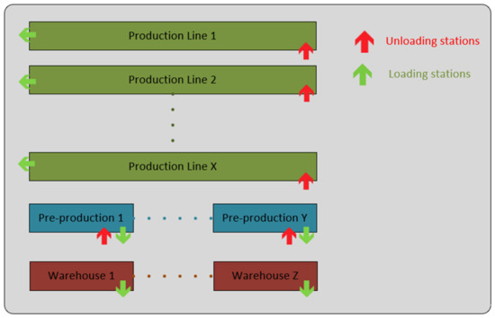
Figure 5.
Simple layout of loading/unloading stations for AGV.
The decision variables are the number of each AGV type in the DT. The following figure illustrates a situation where a collapse of the whole transport system occurred. One AGV trailer blocks another AGV conveying parts to another production line—see Figure 6.
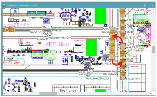
Figure 6.
Sample of AGV collapse.
The optimisation process of the AGV transport is to utilise the tractors with trailers (conveying the small and big parts from the warehouse and the finished products from the production lines) at maximum capacity. The aim is also to utilise all the production lines. The objective function is composed of the following function definitions (the average use of the production lines is superior to the average use of the trains using the coefficients in the objective function):
where
- denotes the resulting objective function (maximisation);
- denotes the number of AGVs of the same type;
- denotes the number of AGVs of different types;
- denotes the utilisation of the i-th production line;
- denotes the number of production lines.
4. Methodology
The concept of Industry 4.0 uses a cyber–physical system (CPS). This system is a computer system in which a mechanism is controlled or monitored by computer-based algorithms.
Assume CPS is a system where its individual parts are managed according to optimised plans. Each essential part of the system is virtually represented in a DT and its operations are managed according to the synchronisation with the other parts of the modelled system (the concrete settings of this simulated part of the production system are represented by the solution candidate). Most simulated objects in the system (parts of the DT) often do not have sufficient computing power to perform their own simulation optimisation. They are interconnected and have the technology to transfer and download data. Therefore, there is no need to perform optimisation using them. The simulation optimisation is performed by remote computers (with sufficient capacity). The settings of the modelled system parameters are sent to the connected physical objects to manage their behaviour.
Simulation optimisation using a DT can be very time consuming. Another problem is the large number of data generated during the simulation experimentation with a DT. The proposed methodology reduces the volume of data generated in the simulation optimisation by combining different approaches used in the global optimisation, programming, and big data techniques. The methodology tries to avoid the problem of generating big data rather than trying to extract information from the huge amount of generated data.
We performed many optimisation experiments in the initial stage of testing, and we confirmed that the selection of the appropriate optimisation method could significantly affect the number of simulation experiments. A common situation in industrial simulation optimisation is that we cannot test all the possible solution candidates in the search space in most cases as it is an NP-hard problem. The next problem is to validate if the optimisation method finds the global minimum or maximum of the objective function of the simulation model (DT). The main advantage of using the optimisation method (especially meta-heuristic methods) is a significant reduction of the number of tested (generated) solution candidates in the simulation optimisation process.
The proposed methodology is described using the AGVs DT representing the transport from the warehouse to the production lines by AGVs. The simulation optimisers running on different servers simulate different variants of the modelled logistic system and use different optimisation techniques to find the best way of conveying the parts with high utilisation of the tractors with trailers.
We developed a system using client–server architecture where the client application controls all the running simulation optimisers on the connected remote computers in parallel. These server simulation optimisers launch the simulation on the simulation software. The server simulation optimiser (or optimisers launched on the computer) can perform the optimisation experiments with a discrete-event simulation model sent by the client application. Each simulation optimiser can use one of the implemented optimisation methods with the setting specified by the client application.
The simulation optimiser, therefore, imitates the decision-making process of an object in an individual part of the simulated system with a defined optimisation strategy, which tries to find its own best possible solution to the simulated problem. For example, the AGV decides how to efficiently convey all the parts to all the locations on the production lines in the shortest amount of time.
The next flowchart shows the several basic phases of the proposed methodology of parallel simulation optimisation—see Figure 7. The principle of running the optimisation experiment using the remote simulation optimiser is described in the flowchart—see Figure 9 in Section 5 Simulation Optimiser.
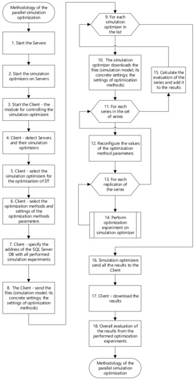
Figure 7.
Flowchart of methodology of the parallel simulation optimisation.
- Step 1 and 2—The simulation run performed on a discrete event simulation model can be time consuming, depending on the difficulty of the discrete event simulation model. The developed simulation optimiser based on client–server architecture allows simulation optimisation experiments to be performed on many remote simulation optimisers—servers. Simulation optimisers are installed on different remote servers. Simulation optimisers perform optimisation experiments with the discrete event simulation model. The simulation optimiser communicates with the client via the assigned port number. The simulation optimiser only waits for the instruction to start the execution of optimisation experiments via the application for remote control of the optimisation experiments. If the version of the running simulation optimiser is older than the current version, the optimiser automatically upgrades to the latest version.
- Step 3, 4, and 5—The application for remote control of optimisation experiments is started on the client’s computer. The application downloads a list of IP addresses of available server computers. The application detects the state of the simulation optimisers. Each IP address lists these attributes of the series: name of the computer performing the optimisation process; status of the simulation optimiser (whether the optimisation experiment is running, ready to run the series, sending files with results, etc.); remaining time to the completion of the current series (the time updates after the completion of each optimisation experiment); remaining time to the completion of all series; index of the currently running series/total number of all series to perform; version of the simulation optimiser application. The user can launch multiple simulation optimisers on the server (depending on the computational capacity of the computer). The server can perform multiple independent series with different simulation models because each running optimiser communicates with the client using its assigned port (depending on the number of the licenses of the simulation software). The next figure shows the GUI of the proposed application for remote control of the optimisation experiments running on the simulation optimisers—see Figure 8.
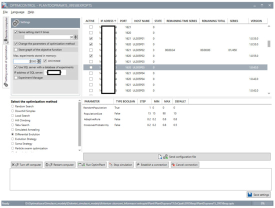 Figure 8. Client application GUI—remote control of simulation optimiser running on servers.
- Step 6—Some methods are very susceptible to the setting of their parameters and this setting greatly affects the behaviour of the method when searching for the global optimum of the objective function. The user can test different parameter settings of the optimisation methods—series.
- Step 7—Simulation optimisers are connected to a remote SQL Server database. This database contains all tested possible solution candidates inside the search space by the remote simulation optimisers (performed simulation experiments with the discrete event simulation model). All simulation optimisers update this SQL server database with performed simulation experiments. The simulation optimiser does not have to perform the simulation run in simulation software, but it only searches for the solution candidate in the databases tested by any other simulation optimiser. The user can also launch another module for collecting the statistics on the use of candidate solutions at the SQL server. We use this module to analyse the relative frequency of using the candidate solutions by the optimisation methods and compare their efficiency of generating new candidate solutions in the optimisation process.
- Step 8—The application for remote control of optimisation experiments sends all necessary files with the settings of the optimisation methods, their parameters, and the simulation model with its concrete settings from the client’s computer to selected simulation optimisers running on servers. The execution of parallel simulation experiments allows the user to distribute simulation models to different computers (using the simulation optimisers) and enhance computing power in the optimisation process with the DT. The use of parallelisation in the simulation (sharing the SQL server database) also eliminates redundant data that would result from simulating the same solution of the modelled problem.
- Step 9 to 12—The performance of the optimisation method is also significantly affected by the settings of the optimisation method parameters; thus, we had to test different settings of the tested optimisation methods to reduce the bad settings of the optimisation methods. The user can also test different settings of the implemented optimisation methods. Each simulation optimiser can use different optimisation methods with different settings of its parameters. The user can set the range of the optimisation method parameters and the simulation optimiser can perform optimisation experiments using all possible settings of the method parameters within the specified range. We can divide the number of simulation experiments as follows:
- Simulation experiment—simulation run of a discrete event simulation model and calculating the objective function value using the outputs from the simulation model.
- Optimisation experiment—performed with a specific optimisation method setting to find the optimum of the objective function (to find the best possible solution to the modelled problem using the digital twin).
- Series—replication of optimisation experiments with a specific optimisation method setting (to test the behaviour of the optimisation method and partial reduction of the wrong settings of the optimisation method parameters). We tested different settings of the optimisation methods and replicated these optimisation experiments with concrete settings of the optimisation method (series) to reduce the influence of random implementation on the optimisation method. The next table shows the tested settings of the implemented optimisation methods, e.g., we tested 470,400,000 different settings of the particle swarm optimisation method—see Table 2, where denotes the dimension of the search space and denotes the number of bits in the gene.
Table 2. Specification of optimisation methods parameters.
- Step 13—The behaviour of the tested optimisation methods is random. We had to repeat many optimisation experiments to identify the pure nature of the optimisation methods (reduce the randomness of the method behaviour) to compare the efficiency of the tested optimisation methods.
- Step 14—The next flowchart shows the basic phases of simulation optimisation running on the simulation optimiser—see Figure 9 in Section 5 Simulation optimiser.
- Step 15—The simulation optimiser performs an evaluation of the series after the completion of each series. The evaluation contains the box plot characteristics of the objective function values of the generated solution candidates (the smallest observation—sample minimum, lower quartile, median, upper quartile, and largest observation—sample maximum) calculated for each series. The evaluation also includes the objective function value of the best-found solution candidates in all optimisation experiments in the series; the range of provided function objective values during the optimisation experiment, and the number of simulation experiments until the termination criterion is met.
- Step 16 to 17—Each simulation optimiser sends all the calculated evaluation results to the client after the completion of all performed series. Sending data also prevents the loss of data from simulation experiments performed on the simulation optimiser if the optimiser fails. These results can be used for the evaluation of the optimisation processes or the evaluation of the behaviour of the methods.
- Step 18—We proposed different criteria which express the success or the failure of the optimisation method in different ways. Each criterion value is between [0,1] and it is calculated from the box plot characteristics—the smallest observation—sample minimum Q1, lower quartile Q2, median Q3, upper quartile Q4, and largest observation—sample maximum Q5. These characteristics are calculated for each series (the setting of the optimisation method parameters)—see Section 6 Evaluation.
5. Simulation Optimiser
The principle of performing the optimisation experiment on the remote simulation optimiser is described in the flowchart—see Figure 9.
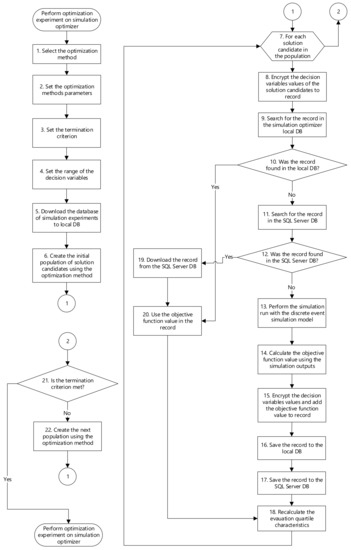
Figure 9.
Flowchart of the optimisation experiment on the parallel simulation optimiser.
- Step 1 and 2—The simulation optimiser selects the optimisation method and sets the range of the optimisation method parameters for the series. This method is set according to the setting sent from the client. If a suitable optimisation method is used, the volume of generated data stored in the memory is significantly reduced.
- Step 3 and 4—The simulation optimiser also sets the termination criteria and the range of decision variables (lower and upper bound of the simulation model input parameters) according to the sent settings. The same termination criteria must be satisfied for each optimisation method in the series.
We specified the first termination criterion—value to reach—because we mapped all the solution candidates in the search space, and we know the best solution for the modelled problem. This best solution candidate represents the global optimum of the objective function. If the optimisation method finds a solution candidate whose objective function value is within the defined tolerated deviation ( in our case) from the objective function value of the global optimum, the optimisation experiment is stopped.
The second termination criterion is the maximum number of simulation runs that the simulation optimiser can perform in the optimisation experiment for each model. We performed many optimisation experiments in the initial stage of testing, and we confirmed that the settings of the optimisation method could significantly affect the performance of the optimisation method. Hence, we tested many different settings of the optimisation methods to reduce the number of bad settings of the optimisation methods parameters and reduce the random nature of the selected optimisation methods (each of the selected methods uses random distribution).
We calculated this maximum number using information entropy known as the Shannon entropy. The number of all possible solutions in the search space is reduced using information entropy [6].
The reduction coefficient is as follows:
where
- denotes the size of the search space—the number of all possible solutions in the search space;
- denotes the coefficient of search space reduction.
The maximum number of simulation runs that it is possible to perform in each optimisation experiment, which is the second termination criterion, is expressed as follows:
We tested this termination criterion using the entropy function on different discrete event simulation models to specify the coefficient. The curve in the chart shows the dependence of the second termination criterion on the number of possible solutions in the search space of the discrete-event simulation model—see Figure 10. The second termination criterion is not much reduced if the number of possible solutions in the search space is small. We set the coefficient according to our optimisation experiments.
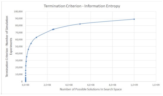
Figure 10.
Derived second termination criterion using information entropy.
To verify this approach, we tested the same settings of the optimisation method on the same models with two specified types of the second termination criterion—the information entropy. Another is commonly used termination criterion which is based on the dimension of the search space (especially in the case of testing functions) as follows:
The following figures show the ability of the implemented optimisation methods to find the known optimum of the objective function on the tested DT when using the following features:
- The information entropy—using the equation——see Figure 11;
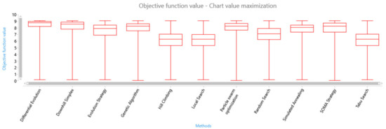 Figure 11. Box plot of solution candidate’s objective function values found by optimisation methods—the second termination criterion using information entropy.
 - The dimension of the search space using the equation——see Figure 12.
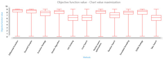 Figure 12. Box plot of solution candidate’s objective function values found by optimisation methods—the second termination criterion using the dimension of the search space.
The difference between the quartiles of the objective values of the solution candidates is minimal in the case of the AGV’s digital twin. We tested this approach with six different discrete event simulation models with different modelled problems.
- Step 5—The simulation optimiser can download the database of the simulation experiments from the SQL servers to its local memory at the start of the optimisation process.
- Step 6—The optimisation method generates the initial population of the solution candidates. We use one fixed solution candidate (starting point) in the initial population to reduce the randomness of the initial searching for the optimum.
- Step 7 and 8—When the simulation optimiser searches for the best solution candidate representing the best setting of discrete-event simulation model parameters, it generates a large volume of data. This volume of data increases with the number of the launched simulation optimisers on the computer. The generated data are stored in internal memory to speed up the optimisation process because many optimisation methods (especially population-based algorithms) use the same individuals that have been generated in previous populations. The problem is mainly related to the maximum size of memory that the simulation optimiser can use (e.g., 32-bit/64-bit application/operating system; the amount of available memory capacity on the computer). A problem could be the lack of computer local memory when storing data of the simulation optimisation run. We implemented the hashing algorithm to reduce the volume of generated data by the optimisation process using the simulation optimiser. The principle of the algorithm is shown in Algorithm 5.
| Algorithm 5: Hashing Algorithm Pseudocode | ||
| Hashing function returning the list of values to reduce the required memory for storing decision variables values | ||
| Input: | List of all decision variables (simulation model input parameters) | |
| DV[i].v | The i-th decision variable value | |
| DV[i].numBits | Number of bits of the i-th decision variable | |
| DV[i].a | Lower bound of the i-th decision variable | |
| DV[i].b | Upper bound of the i-th decision variable | |
| DV[i].step | Step (difference between two following values) of the i-th decision variable | |
| Data: | Returns the number of decimal places | |
| ToInt | Converts a specified value to 32-bit signed integer | |
| ToBin | Converts a specified value to binary number (string data type) | |
| ToStr | Converts a specified value to its equivalent string representation | |
| ToInt64 | Converts a specified string to 64-bit signed integer | |
| SubString | Returns a new string containing the section of the current string starting at index position Start and containing the specified number of characters | |
| intNum | Integer number (local variable) | |
| binNum | Binary number (local variable-string data type) | |
| FinalBinNum | Binary value of the converted number (string data type) | |
| Output: | List of all hashed values of the converted decision variables values | |
| 1 begin 2 3 //Go through all decision variables 4 for do begin 5 if then 6 if then //Concatenate sign bit to string binary number 7 8 else 9 //Conversion of the real number to integer number 10 //Convert integer number to string binary number 11 //Pad ‘0′ to string binary number 12 for do 13 //Final binary number 14 15 end; //Clear the output list 16 //Split the string to 64 parts 17 for do //Add converted decision variables values to list 18 19 result ; 20 end; | ||
Each solution candidate in the search space of the AGVs DT contains 15 decision variables (values of discrete event simulation model input parameters) and the objective function value of the solution candidate. If we use the standard approach for storing the database record, then we would need 15 + 1 fields (15 values of double data type—the storage size of double is 8 bytes; 1 field of real data type for objective function value—the storage size of real is 4 bytes). We use the hashing algorithm to encrypt all the values of decision variables of the solution candidate to one big integer value (bigint data type) that takes 8 bytes. Thus, we saved 15 times more space for each record containing the settings of the AGVs DT decision variables used for the performed simulation experiment.
- Step 9–12 and 19–20—The simulation optimisers can also download the record (encrypted data) from the remote database including all simulation experiments performed with the discrete event simulation model. The simulation optimiser does not have to perform the simulation run in simulation software, but it only searches for the simulation experiment in the local memory of the simulation optimiser. It can also search for the solution candidate (record) in the SQL server database if the local memory does not contain this solution candidate. The simulation optimiser does not have to perform the simulation run in simulation software, but it only searches for the solution candidate in the internal memory of all the solution candidates. The simulation experiment with AGVs DT takes about 10 s. If the simulation experiment was performed by any other simulation optimiser, the execution of the SQL query including loading the record representing the simulation experiment takes only 0.001 s. As we use the hashing algorithm, a SQL query with only one parameter value was used to find a simulation experiment with AGVs DT instead of searching for 15 parameter values (the SQL query would have to contain 15 conjunctive conditions, which means multiple slowdowns). The next advantage is indexing this field for faster searching of the database record.
- Step 13 and 14—If the local server or the remote SQL Server database does not contain the needed solution candidate, the simulation optimiser generates a candidate solution. This candidate solution represents the settings of the simulation model input parameters. The simulation optimiser launches the simulation run on the simulation software. We used the Tecnomatix Plant Simulation software developed by Siemens PLM Software. The simulation optimiser calculates the objective function value of this candidate solution using the simulation outputs.
- Step 15—The values of the decision variables of the solution candidate and its objective function value are encrypted by the hashing method to reduce the data volume. The hashing method supports the possibility of indexing records using the SQL server to speed up the search of records in the database while minimising memory requirements.
- Step 16 and 17—One way of speeding up the optimisation process is by storing the data generated by the optimisation process in the internal memory allocated to the simulation optimiser. We found that the optimisation algorithms often use the same solution candidates to map the objective function landscape (searching for the path to the optimum of the objective function). This fact can be used to speed up the optimisation process and reduce the data stored in the memory of the simulation optimiser. The simulation optimisers are connected to the SQL server database containing the records—the tested solution candidates and their objective values. Each simulation optimiser provides the possibility of downloading or uploading the data from the simulation experiment to the SQL server. The record is stored in the local database and to the SQL server database if the database does not contain this specific record (another simulation optimiser could perform the same simulation experiment and sends the record to the SQL Server database at the same time). This reduces the duplicated simulation experiments in the SQL server database. The simulation optimiser does not download the same simulation experiments in the initial stage of the simulation optimisation of the DT. Each DT has its own database of simulation experiments. The developed application supports managing the volume of data (generated by previous optimisation processes) held in the memory by setting the following options:
- No previously performed optimisation experiments are held in the memory—the simulation optimiser detects if the SQL server contains a solution candidate, that is, a record containing the performed simulation run (the concrete settings of the simulation model input parameters and the objective function value calculated according to the output of the simulation run with concrete settings). If this database contains this record, the simulation optimiser downloads these encrypted data by the hashing algorithm and decrypts them; otherwise, the simulation is run with the concrete settings of the simulation model input parameters.
- The simulation optimiser stores the specified number of records (executed simulation runs and calculated objective function values) in the local memory—this option is used when the simulation optimiser can use the limited available memory. The optimiser scans its internal computer memory first to find a specific record (the concrete settings of the simulation model input parameters). If it does not find this record in the internal memory, it searches the SQL server for this record. If the record is not found, the simulation optimiser runs the simulation experiment with the concrete settings of the simulation model input parameters.
- The simulation optimiser stores all the performed optimisation experiments (all records)—the logic is the same as the previous variant except that all the simulation runs in all optimisation experiments are held in the computer’s memory. The simulation optimiser downloads all records from the SQL server database. This approach will cause a certain time delay before the first simulation run is started, but it will save time spent on the communication between the SQL server and the simulation optimiser.
- Step 18—The simulation optimiser continuously displays the state of the optimisation experiment. It displays the value of the objective function of the proposed solution candidate; decision variables values (the settings of the simulation model input parameters of the proposed solution); the value of the objective function and the number of the simulation experiments in which the best solution candidate was found by the optimisation method; the value of the objective function of the current solution; the number of the current simulation experiment; simulation experiment computation time; the number of loaded/saved simulation experiments in the internal or external database, etc.; see Figure 13. The simulation optimiser also calculates the evaluation box plot characteristics of objective function values of the best-found solution candidates, all generated solution candidates, and the number of performed simulation experiments for each series.
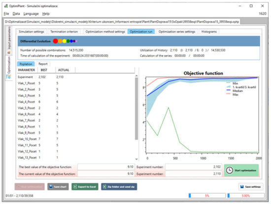 Figure 13. Simulation optimiser GUI—optimisation experiment with AGVs DT.
- Step 21—If any of the termination criteria are met, the optimisation experiment is terminated.
6. Evaluation
Many research papers use the mean and the standard deviation to evaluate the performance of the optimisation methods. This evaluation criterion is sufficient for commonly used testing functions, e.g., De Jong’s function, Rosenbrock’s function, Ackley’s function, etc. [78] where the global optimum is known.
We proposed different evaluation criteria [33]. Each criterion value is between 0 and 1, and it is calculated from the box plot characteristics for the smallest observation, namely, sample minimum Q1, lower quartile Q2, median Q3, and upper quartile Q4, and for the largest observation, sample maximum Q5. These characteristics are calculated for each series, defining the setting of the optimisation method parameters. As we wanted to compare the efficiency of the implemented optimisation methods, we mapped all the solution candidates in the search space to identify the global optimum of the objective function of the AGV’s DT.
6.1. Quality of the Found Solution Candidate
Figure 11 shows the calculated quartiles characteristics from all the performed series (replicated optimisation experiments with the concrete setting of the optimisation method) of all the optimisation methods performed on the AGV’s digital twin. There are four winners in this category—differential evolution, downhill simplex, self-organising migrating algorithm (SOMA), and genetic algorithm.
6.2. The Speed in Finding a Solution Candidate
The speed of the optimisation method in finding a solution candidate is the number of performed simulation experiments until the optimum/best solution candidate (suboptimum) was found in each series. If the optimisation method is effective, the volume of generated data (solution candidates) is quite small. The local search seems similar to the fastest optimisation method, but this method does not find the global optimum of the AGV’s simulation model—see Figure 14. Other methods such as differential evolution, downhill simplex, and simulated annealing are also fast. Some methods (especially evolutionary computation methods) need to perform a large number of simulation experiments (representing individuals in the population) ensuring the escape from the local extremes of the objective function. This feature is particularly suitable for the multimodal objective function, but it generates a large volume of data.
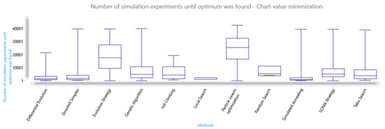
Figure 14.
Box plot of the speed in finding a global optimum of the objective function.
The dimension of the search space is 15. The problem is how to display the objective function landscape containing millions of solution candidates. We calculated the relative frequencies of the mapped objective function values of the solution candidates considering the smaller intervals of the objective function values—see Figure 15. The objective function of the AGV model is maximised, and the higher values of relative frequencies with higher values of the objective function predominate in the chart. The probability of finding an acceptable solution is good. The relative frequencies of the objective function values (how often the objective function values occur within different ranges of objective function values) can also be used when we do not map all the solution candidates and their objective function values in the whole search space.
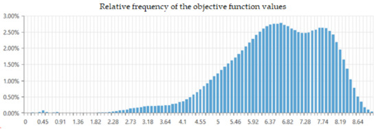
Figure 15.
The percentage of relative frequency of the objective function values.
The series also contains the solution candidates whose objective function values are not the same as the objective function of the global optimum (we accepted the solution candidates as the global optimum if their objective function value is within the defined tolerated deviation ). The next box plot chart shows the number of simulation experiments until the suboptimum was found–see Figure 16. The box plot chart shows big differences in the efficiency of searching for the optimum. differential evolution, downhill simplex, and simulated annealing are the winners in the AGV model.
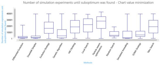
Figure 16.
Box plot of the speed in finding a suboptimum of the objective function.
We proposed other criteria, i.e., quality of solution candidates using the distances of quartiles between optimum and suboptimum or the quartiles of the objective function values of the solution candidates. The other criterion is the convergence of the objective function values of the generated solution candidates in the series. We calculated the weighted sum of the proposed evaluation criteria using the specified weights for each criterion. The next box plot chart shows the weighted sum of the proposed evaluation criteria calculated for each series—see Figure 17. Differential evolution, downhill simple, and self-organizing migrating algorithm (SOMA) are effective methods for finding the global optimum in the search space of the AGV model.
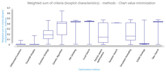
Figure 17.
Box plot of solution candidate’s objective function values found by optimisation methods—the second termination criterion using the dimension of the search space.
6.3. Settings of the Optimisation Methods
Many of the optimisation methods are very sensitive to the settings of their parameters. The application we developed for evaluating the series also allows the user to filter 25% of the best series (the settings of the optimisation method parameters) using the calculated weighted sum for each series.
The next box plot chart shows the calculated characteristics of the number of simulation experiments until the suboptimum was found—see Figure 18. If we compare this box plot chart with the chart in Figure 16, some methods are sensitive to bad settings of their parameters. Simulated annealing, differential evolution, and downhill simplex do not need a large number of simulation experiments to find the suboptimum.
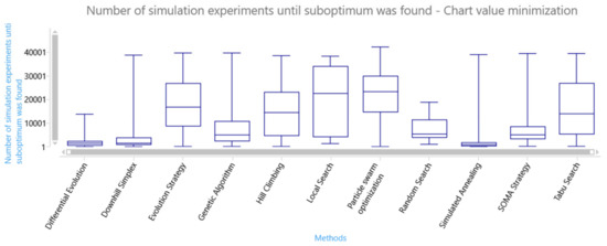
Figure 18.
Box plot of the speed of finding a suboptimum of the objective function—25% of the best series.
If we select the best settings of the differential evolution parameters (best series) for the AGV model and replicate this series 30 times, we can visualise the percentage frequency of the objective function values of the solution candidates generated by this method. If we compare the following box plot chart (see Figure 19) with the percentage of the relative frequency of the objective function values of all the solution candidates in the whole search space (see Figure 15), a radical reduction in unnecessarily generated solutions and a fast targeting of the area of the optimal solution are obvious.
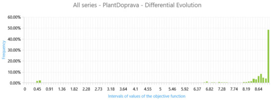
Figure 19.
The percentage of the frequency of the objective function values of solution candidates generated by the differential evolution.
7. Conclusions
The goal of our research is to propose a methodology for reducing the volume of data generated in a simulation optimisation, performed with a DT and created in accordance with the Industry 4.0 concept. This methodology is validated using applications developed for controlling the execution of parallel simulation experiments (using client–server architecture developed to distribute simulation models to different computers and enhance computing power) with the DT by the simulation optimiser and an application developed for evaluating the optimisation experiments using different criteria calculating the information from the statistical data. The paper presents some approaches for reducing the data used for simulation optimisation, e.g., parallel optimisation, hashing the data, using a server with data obtained from remote simulation optimisers, using different modified optimisation methods, and the evaluation of the series used for finding the appropriate setting of method parameters. This methodology attempts to prevent the generation of unnecessary data during the optimisation process with the DT rather than mining information from large amounts of data generated by the optimisation methods. We found that the behaviour of the optimisation methods strongly depends on the objective function landscape. The efficiency of the differential evolution method is high, due to the relatively simple objective function landscape of the AGV’s digital twin.
Our future work will focus on using a neural network to approximate the objective function values of generated candidate solutions and compare the effectiveness of this method with metaheuristic algorithms.
The proposed methodology is designed for optimisation with discrete simulation models, not for continuous simulation models.
Author Contributions
Conceptualization, P.R., Z.U. and M.M.; methodology, P.R.; software, Z.U.; validation, Z.U. and P.R.; formal analysis, P.R., Z.U. and M.M.; investigation, M.M.; resources, P.R., Z.U. and M.M.; data curation, Z.U. and P.R.; writing—original draft preparation, P.R.; writing—review and editing, P.R., Z.U. and M.M.; visualization, P.R., Z.U. and M.M.; supervision, Z.U.; project administration, P.R.; funding acquisition, P.R. All authors have read and agreed to the published version of the manuscript.
Funding
This paper was created with the subsidy of the project SGS-2021-028 ‘Developmental and training tools for the interaction of man and the cyber–physical production system’ carried out with the support of the Internal Grant Agency of the University of West Bohemia.
Institutional Review Board Statement
Not applicable.
Informed Consent Statement
Not applicable.
Data Availability Statement
https://drive.google.com/file/d/1NAddbWU6XWet22oTDCQkHP6dGlX9Whwr/view?usp=sharing (accessed on 20 July 2021).
Conflicts of Interest
The authors declare no conflict of interest.
References
- Hartmann, D.; Van der Auweraer, H. Digital Twins. In Progress in Industrial Mathematics: Success Stories; Cruz, M., Parés, C., Quintela, P., Eds.; Springer International Publishing: Cham, Germany, 2021; Volume 5, pp. 3–17. [Google Scholar] [CrossRef]
- Fryer, T. Digital Twin—Introduction. This is the age of the Digital Twin. Eng. Technol. 2019, 14, 28–29. [Google Scholar] [CrossRef]
- Andronas, D.; Kokotinis, G.; Makris, S. On modelling and handling of flexible materials: A review on Digital Twins and planning systems. Procedia CIRP 2021, 97, 447–452. [Google Scholar] [CrossRef]
- Rao, S.V. Using a Digital Twin in Predictive Maintenance. J. Pet. Technol. 2020, 72, 42–44. [Google Scholar] [CrossRef]
- Liljaniemi, A.; Paavilainen, H. Using Digital Twin Technology in Engineering Education—Course Concept to Explore Benefits and Barriers. Open Eng. 2020, 10, 377–385. [Google Scholar] [CrossRef]
- Lv, Z.; Chen, D.; Lou, R.; Alazab, A. Artificial intelligence for securing industrial-based cyber–physical systems. Future Gener. Comput. Syst. 2021, 117, 291–298. [Google Scholar] [CrossRef]
- Vogel-Heuser, B.; Lee, J.; Leitão, P. Agents enabling cyber-physical production systems. at-Automatisierungstechnik 2015, 63, 777–789. [Google Scholar] [CrossRef] [Green Version]
- Tao, F.; Qi, Q.; Wang, L.; Nee, A.Y.C. Digital Twins and Cyber–Physical Systems toward Smart Manufacturing and Industry 4.0: Correlation and Comparison. Engineering 2019, 5, 653–661. [Google Scholar] [CrossRef]
- Uhlemann, T.H.-J.; Lehmann, C.; Steinhilper, R. The Digital Twin: Realizing the Cyber-Physical Production System for Industry 4.0. Procedia CIRP 2017, 61, 335–340. [Google Scholar] [CrossRef]
- Lee, J.; Bagheri, B.; Kao, H.-A. Recent Advances and Trends of Cyber-Physical Systems and Big Data Analytics in Industrial Informatics. In Proceedings of the International Conference on Industrial Informatics, Porto Alegre, Brazil, 27–30 July 2014. [Google Scholar] [CrossRef]
- Lu, Y.; Liu, C.; Wang, K.I.-K.; Huang, H.; Xu, X. Digital Twin-driven smart manufacturing: Connotation, reference model, applications and research issues. Robot. Comput. Manuf. 2020, 61, 101837. [Google Scholar] [CrossRef]
- Zhang, Y.; Ren, S.; Liu, Y.; Si, S. A big data analytics architecture for cleaner manufacturing and maintenance processes of complex products. J. Clean. Prod. 2017, 142, 626–641. [Google Scholar] [CrossRef] [Green Version]
- Gandomi, A.; Haider, M. Beyond the hype: Big data concepts, methods, and analytics. Int. J. Inf. Manag. 2015, 35, 137–144. [Google Scholar] [CrossRef] [Green Version]
- Alwan, H.B.; Ku-Mahamud, K.R. Big data: Definition, characteristics, life cycle, applications, and challenges. IOP Conf. Ser. Mater. Sci. Eng. 2020, 769, 012007. [Google Scholar] [CrossRef]
- Kendzierskyj, S.; Jahankhani, H.; Jamal, A.; Jimenez, J.I. The Transparency of Big Data, Data Harvesting and Digital Twins; Jahankhani, H., Kendzierskyj, S., Jamal, A., Epiphaniou, G., Al-Khateeb, H., Eds.; Springer International Publishing: Cham, Germany, 2019; pp. 139–148. [Google Scholar] [CrossRef]
- Da Xu, L.; Duan, L. Big data for cyber physical systems in industry 4.0: A survey. Enterp. Inf. Syst. 2019, 13, 148–169. [Google Scholar] [CrossRef]
- He, W.; Da Xu, L. Integration of Distributed Enterprise Applications: A Survey. IEEE Trans. Ind. Inform. 2012, 10, 35–42. [Google Scholar] [CrossRef]
- Vieira, A.A.; Dias, L.M.; Santos, M.Y.; Pereira, G.A.B.; Oliveira, J.A. On the use of simulation as a Big Data semantic validator for supply chain management. Simul. Model. Pract. Theory 2020, 98, 101985. [Google Scholar] [CrossRef]
- Cheng, S.; Liu, B.; Ting, T.O.; Qin, Q.; Shi, Y.; Huang, K. Survey on data science with population-based algorithms. Big Data Anal. 2016, 1, 35. [Google Scholar] [CrossRef] [Green Version]
- Amaran, S.; Sahinidis, N.V.; Sharda, B.; Bury, S.J. Simulation optimization: A review of algorithms and applications. Ann. Oper. Res. 2016, 240, 351–380. [Google Scholar] [CrossRef] [Green Version]
- Xu, J.; Huang, E.; Chen, C.-H.; Lee, L.H. Simulation Optimization: A Review and Exploration in the New Era of Cloud Computing and Big Data. Asia-Pac. J. Oper. Res. 2015, 32, 1550019-1–1550019-34. [Google Scholar] [CrossRef]
- Alrabghi, A.; Tiwari, A.; Savill, M. Simulation-based optimisation of maintenance systems: Industrial case studies. J. Manuf. Syst. 2017, 44, 191–206. [Google Scholar] [CrossRef] [Green Version]
- Longo, C.S.; Fantuzzi, C. Simulation and optimization of industrial production lines. at-Automatisierungstechnik 2018, 66, 320–330. [Google Scholar] [CrossRef]
- Shahbazi, S.; Sajadi, S.M.; Jolai, F. A Simulation-Based Optimization Model for Scheduling New Product Development Projects in Research and Development Centers. Iranian J. Manag. Stud. 2017, 10. [Google Scholar] [CrossRef]
- Van Der Auweraer, H.; Anthonis, J.; De Bruyne, S.; Leuridan, J. Virtual engineering at work: The challenges for designing mechatronic products. Eng. Comput. 2012, 29, 389–408. [Google Scholar] [CrossRef] [Green Version]
- Tasoglu, G.; Yildiz, G. Simulated annealing based simulation optimization method for solving integrated berth allocation and quay crane scheduling problems. Simul. Model. Pract. Theory 2019, 97, 101948. [Google Scholar] [CrossRef]
- Grzybowska, H.; Kerferd, B.; Gretton, C.; Travis Waller, S. A simulation-optimisation genetic algorithm approach to product allocation in vending machine systems. Expert Syst. Appl. 2020, 145, 113110. [Google Scholar] [CrossRef]
- Bovim, T.R.; Christiansen, M.; Gullhav, A.N.; Range, T.M.; Hellemo, L. Stochastic master surgery scheduling. Eur. J. Oper. Res. 2020, 285, 695–711. [Google Scholar] [CrossRef]
- Rouky, N.; Abourraja, M.N.; Boukachour, J.; Boudebous, D.; Alaoui, A.E.H.; El Khoukhi, F. Simulation optimization based ant colony algorithm for the uncertain quay crane scheduling problem. Int. J. Ind. Eng. Comput. 2019, 10, 111–132. [Google Scholar] [CrossRef]
- Yang, T.; Kuo, Y.; Chang, I. Tabu-search simulation optimization approach for flow-shop scheduling with multiple processors—A case study. Int. J. Prod. Res. 2004, 42, 4015–4030. [Google Scholar] [CrossRef]
- Hong, L.J.; Nelson, B.L. A brief introduction to optimization via simulation. In Proceedings of the 2009 Winter Simulation Conference (WSC), Austin, TX, USA, 13–16 December 2009; pp. 75–85. [Google Scholar] [CrossRef] [Green Version]
- Trigueiro de Sousa Junior, W.; Barra Montevechi, J.A.; de Carvalho Miranda, R.; Teberga Campos, A. Discrete simulation-based optimization methods for industrial engineering problems: A systematic literature review. Comput. Ind. Eng. 2019, 128, 526–540. [Google Scholar] [CrossRef]
- Raska, P.; Ulrych, Z. Methodology for evaluating optimization experiments. In Proceedings of the 32nd European Modeling and Simulation Symposium, EMSS 2020, Athens, Greece, 16–18 September 2020. [Google Scholar] [CrossRef]
- Nelder, J.A.; Mead, R. A Simplex Method for Function Minimization. Comput. J. 1965, 7, 308–313. [Google Scholar] [CrossRef]
- Maehara, N.; Shimoda, Y. Application of the genetic algorithm and downhill simplex methods (Nelder–Mead methods) in the search for the optimum chiller configuration. Appl. Therm. Eng. 2013, 61, 433–442. [Google Scholar] [CrossRef]
- Weise, T. Global Optimization Algorithms–Theory and Application. 2009. Available online: http://www.it-weise.de (accessed on 2 February 2011).
- Raska, P.; Ulrych, Z. Comparison of optimisation methods tested on testing functions and discrete event simulation models. Int. J. Simul. Process. Model. 2015, 10, 279. [Google Scholar] [CrossRef]
- Monticelli, A.J.; Romero, R.; Asada, E. Fundamentals of Tabu Search. In Modern Heuristic Optimization Techniques; Wiley-IEEE Press: Piscataway, NJ, USA, 2007; pp. 101–122. [Google Scholar]
- Dréo, J.; Pétrowski, A.; Taillard, E. Metaheuristics for Hard Optimization; Springer: Berlin/Heidelberg, Germany, 2006. [Google Scholar] [CrossRef]
- Monticelli, A.J.; Romero, R.; Asada, E. Fundamentals of Simulated Annealing. In Modern Heuristic Optimization Techniques: Theory and Applications to Power Systems; Wiley-IEEE Press: Hoboken, NJ, USA, 2007; pp. 123–146. [Google Scholar] [CrossRef]
- Gonzalez, T.F. Handbook of Approximation Algorithms and Metaheuristics; Chapman and Hall/CRC: New York, NY, USA, 2007; 1432p. [Google Scholar] [CrossRef]
- Storn, R.; Price, K.V. Differential Evolution–A Simple and Efficient Heuristic for global Optimization over Continuous Spaces. J. Glob. Optim. 1997, 11, 341–359. [Google Scholar] [CrossRef]
- Eltaeib, T.; Mahmood, A. Differential Evolution: A Survey and Analysis. Appl. Sci. 2018, 8, 1945. [Google Scholar] [CrossRef] [Green Version]
- Zelinka, I. SOMA—Self-organizing Migrating Algorithm. In Studies in Computational Intelligence; Springer: Cham, Germany, 2016. [Google Scholar] [CrossRef]
- Zelinka, I.; Davendra, D.D.; Senkerik, R.; Pluhacek, M. Investigation on evolutionary predictive control of chemical reactor. J. Appl. Log. 2015, 13, 156–166. [Google Scholar] [CrossRef]
- Li, Y.-L.; Zhan, Z.-H.; Gong, Y.-J.; Chen, W.-N.; Zhang, J.; Li, Y. Differential Evolution with an Evolution Path: A DEEP Evolutionary Algorithm. IEEE Trans. Cybern. 2014, 45, 1798–1810. [Google Scholar] [CrossRef] [PubMed] [Green Version]
- Pant, M.; Zaheer, H.; Garcia-Hernandez, L.; Abraham, A. Differential Evolution: A review of more than two decades of research. Eng. Appl. Artif. Intell. 2020, 90, 103479. [Google Scholar] [CrossRef]
- Zelinka, I.; Snasel, V.; Abraham, A. (Eds.) Handbook of Optimization; Springer: Berlin/Heidelberg, Germany, 2013; Volume 38. [Google Scholar] [CrossRef]
- Rechenberg, I. Cybernetic Solution Path of an Experimental Problem (Kybernetische Lösungsansteuerung Einer Experimentellen Forschungsaufgabe). In Evolutionary Computation: The Fossil Record; Wiley-IEEE Press: Hoboken, NJ, USA, 1998. [Google Scholar] [CrossRef]
- Bäck, T.; Foussette, C.; Krause, P. Contemporary Evolution Strategies. Nat. Comput. Ser. 2013, 47. [Google Scholar] [CrossRef]
- Beyer, H.-G.; Schwefel, H.-P. Evolution strategies—A comprehensive introduction. Nat. Comput. 2002, 1, 3–52. [Google Scholar] [CrossRef]
- Hansen, N.; Ostermeier, A.; Gawelczyk, A. On the Adaptation of Arbitrary Normal Mutation Distributions in Evolution Strategies: The Generating Set Adaptation. In Proceedings of the Sixth International Conference on Genetic Algorithms, San Francisco, CA, USA, 15–19 July 1995. [Google Scholar]
- Meyer-Nieberg, S.; Beyer, H.-G. Self-Adaptation in Evolutionary Algorithms. Stud. Comput. Intell. 2007, 47–75. [Google Scholar] [CrossRef]
- Akhtar, J.; Awais, M.M.; Koshul, B.B. Evolutionary Algorithms based on non-Darwinian theories of evolution. In Proceedings of the 2008 IEEE Congress on Evolutionary Computation (IEEE World Congress on Computational Intelligence), Hong Kong, China, 1–6 June 2008; pp. 2554–2560. [Google Scholar] [CrossRef]
- Beyer, H.-G.; Sendhoff, B. Covariance Matrix Adaptation Revisited—The CMSA Evolution Strategy. In Lecture Notes in Computer Science (Including Subseries Lecture Notes in Artificial Intelligence and Lecture Notes in Bioinformatics); Springer: Berlin/Heidelberg, Germany, 2008. [Google Scholar] [CrossRef]
- Igel, C.; Suttorp, T.; Hansen, N. Steady-State Selection and Efficient Covariance Matrix Update in the Multi-Objective CMA-ES. In Evolutionary Multi-Criterion Optimization; Springer: Berlin/Heidelberg, Germany, 2007; Volume 4403, pp. 171–185. [Google Scholar] [CrossRef]
- Müller, C.L.; Sbalzarini, I.F. Gaussian Adaptation. In Lecture Notes in Computer Science (Including Subseries Lecture Notes in Artificial Intelligence and Lecture Notes in Bioinformatics); Springer: Berlin/Heidelberg, Germany, 2010. [Google Scholar] [CrossRef]
- Hansen, N.; Ostermeier, A. Convergence Properties of Evolution Strategies with the Derandomized Covariance Matrix Adaptation: The (Mu/Mu_I, Lambda)-CMA-ES. In Proceedings of the 5th European Congress on Intelligent Techniques and Soft Computing, Aachen, Germany, 8–11 September 1997. [Google Scholar]
- Jastrebski, G.; Arnold, D. Improving Evolution Strategies through Active Covariance Matrix Adaptation. In Proceedings of the 2006 IEEE International Conference on Evolutionary Computation, Vancouver, BC, Canada, 16–21 July 2006. [Google Scholar] [CrossRef]
- Tripathy, A.; Schwefel, H.-P. Numerical Optimization of Computer Models. J. Oper. Res. Soc. 1982, 33, 1166. [Google Scholar] [CrossRef]
- Beyer, H.-G. Toward a Theory of Evolution Strategies: Self-Adaptation. Evol. Comput. 1995, 3, 311–347. [Google Scholar] [CrossRef]
- Matsumura, Y.; Ohkura, K.; Ueda, K. Advantages of global discrete recombination in (μ/μ,λ,)-evolution strategies. In Proceedings of the 2002 Congress on Evolutionary Computation, CEC 2002, Honolulu, HI, USA, 12–17 May 2002. [Google Scholar] [CrossRef]
- Geyer, H.; Ulbig, P.; Schulz, S. Verschachtelte Evolutionsstrategien Zur Optimierung Nichtlinearer Verfahrenstechnischer Regressions-Probleme. Chem. Ing. Tech. 2000, 72, 369–373. [Google Scholar] [CrossRef]
- Rechenberg, I. Evolutionsstrategie—Optimieren wie in der Natur. Technik und Natur 1994, 227–244. [Google Scholar] [CrossRef]
- Raska, P.; Ulrych, Z. Testing different evolution strategy selection strategies. MM Sci. J. 2018, 2018, 2290–2299. [Google Scholar] [CrossRef] [Green Version]
- Eberhart, R.; Kennedy, J. New Optimizer Using Particle Swarm Theory. In Proceedings of the International Symposium on Micro Machine and Human Science, Nagoya, Japan, 4–6 October 1995. [Google Scholar] [CrossRef]
- Parrish, J.K.; Hamner, W.M. (Eds.) Animal Groups in Three Dimensions; Cambridge University Press: Cambridge, UK, 1997. [Google Scholar] [CrossRef]
- Wang, D.; Tan, D.; Liu, L. Particle swarm optimization algorithm: An overview. Soft Comput. 2018, 22, 387–408. [Google Scholar] [CrossRef]
- Marini, F.; Walczak, B. Particle swarm optimization (PSO). A tutorial. Chemom. Intell. Lab. Syst. 2015, 149, 153–165. [Google Scholar] [CrossRef]
- Piotrowski, A.P.; Napiorkowski, J.; Piotrowska, A.E. Population size in Particle Swarm Optimization. Swarm Evol. Comput. 2020, 58, 100718. [Google Scholar] [CrossRef]
- Bonyadi, M.R.; Michalewicz, Z. Particle Swarm Optimization for Single Objective Continuous Space Problems: A Review. Evol. Comput. 2017, 25, 1–54. [Google Scholar] [CrossRef]
- Nagpal, R.; Singh, P.; Garg, B.P. Smart Particle Swarm Optimization. In Proceedings of the 2021 International Conference on Computing, Communication, and Intelligent Systems (ICCCIS), Greater Noida, India, 19–20 February 2021. [Google Scholar] [CrossRef]
- Xu, G.; Cui, Q.; Shi, X.; Ge, H.; Zhan, Z.-H.; Lee, H.P.; Liang, Y.; Tai, R.; Wu, C. Particle swarm optimization based on dimensional learning strategy. Swarm Evol. Comput. 2019, 45, 33–51. [Google Scholar] [CrossRef]
- Tawhid, M.A.; Dsouza, K.B. Hybrid binary bat enhanced particle swarm optimization algorithm for solving feature selection problems. Appl. Comput. Inform. 2018, 16, 117–136. [Google Scholar] [CrossRef]
- Zhan, Z.-H.; Wang, Z.-J.; Jin, H.; Zhang, J. Adaptive Distributed Differential Evolution. IEEE Trans. Cybern. 2020, 50, 4633–4647. [Google Scholar] [CrossRef] [PubMed]
- Raska, P.; Ulrych, Z. Testing Different Particle Swarm Optimization Strategies. In Proceedings of the 30th International Business Information Management Association Conference, IBIMA 2017—Vision 2020: Sustainable Economic development, Innovation Management, and Global Growth, Madrid, Spain, 8–9 November 2017; Volume 2017. [Google Scholar]
- Raska, P.; Ulrych, Z. Evaluation of a Self-Organizing Migrating Algorithm applied to discrete event simulation optimization. In Proceedings of the 31st European Modeling and Simulation Symposium, EMSS 2019, Lisbon, Portugal, 18–20 September 2019. [Google Scholar]
- Arora, K.; Kumar, A.; Kamboj, V.K.; Prashar, D.; Jha, S.; Shrestha, B.; Joshi, G.P. Optimization Methodologies and Testing on Standard Benchmark Functions of Load Frequency Control for Interconnected Multi Area Power System in Smart Grids. Mathematics 2020, 8, 980. [Google Scholar] [CrossRef]
Publisher’s Note: MDPI stays neutral with regard to jurisdictional claims in published maps and institutional affiliations. |
© 2021 by the authors. Licensee MDPI, Basel, Switzerland. This article is an open access article distributed under the terms and conditions of the Creative Commons Attribution (CC BY) license (https://creativecommons.org/licenses/by/4.0/).