Simulation of Fluid Dynamics Monitoring Using Ultrasonic Measurements

Featured Application

Monitoring of liquid metal flows by ultrasounds.

Abstract

The simulation of the propagation of ultrasonic waves in a moving fluid will improve the efficiency of the ultrasonic flow monitoring and that of the in-service monitoring for various reactors in several industries. The most recent simulations are mostly limited to 3D representations of the insonified volume but without really considering the temporal aspect of the flow. The advent of high-performance computing (HPC) now makes it possible to propose the first 4D simulations, with the representation of the inspected medium evolving over time. This work is based on a highly accurate double simulation. A first computational fluid dynamics (CFD) simulation, performed in previous work, described the fluid medium resulting from the mixing of hot jets in a cold opaque fluid. There have been many sensor developments over the years in this domain, as ultrasounds are the only method able to give information in an opaque medium. The correct design of these sensors, as well as the precise and confident analysis of their measurements, will progress with the development of the modeling of wave propagation in such a medium. An important parameter to consider is the flow temperature description, as a temperature gradient in the medium deflects the wave path and may sometimes cause its division. We develop a 4D wave propagation simulation in a very realistic, temporally fluctuating medium. A high-performance simulation is proposed in this work to include an ultrasonic source within the medium and to calculate the wave propagation between a transmitter and a receiver. The analysis of the wave variations shows that this through-transmission setup can track the jet mixing time variations. The steps needed to achieve these results are described using the spectral-element-based numerical tool SPECFEM3D. It is shown that the low-frequency fluctuation of the liquid metal flow can be observed using ultrasonic measurements.

1. Introduction

Flow monitoring is of importance for many applications involving various liquids and gases. There exist some methods to characterize flows using global measurements effective in many industrial situations [1]. Many technologies use pressure variations to deduce flow rate. When the fluid has conductive properties, other technologies use electromagnetic measurements. In many cases, a precise analysis of the velocity distribution in the flow is required. When optical paths are possible, a classical solution consists of making Doppler measurements with particles floating in the fluid. Major developments in three-dimensional velocity field measurements using the tomographic particle image velocimetry (PIV) technique have taken place in past years [2]. When the flow is opaque or when it cannot be optically observed directly, then ultrasonic solutions are often implemented. In the case of liquid metals, the floating particles may be impurities (such as metallic inclusions or oxide films), and ultrasonic measurements are also used to analyze the purity of liquid metal [3,4]. There are also studies in magnetohydrodynamics (MHDs) where flows, in metallic melts, can be driven by magnetic fields. The study of turbulent melt flows requires 2D flow mapping at a frame rate of several hertz. Thieme et al. developed an ultrasound array doppler velocimeter (UADV) using linear arrays of large piezoelectric elements. They demonstrated they can detect the transition from laminar flow to turbulent flow [5]. In such media, simultaneously monitoring temperatures in the flow and the fluid dynamics presents the most difficulties. Zürner et al. proposed to combine multiple crossing ultrasound beam lines and an array of thermocouples to realize a 3D characterization of the complex dynamics in a cylindrical convection cell that is filled with the liquid metal alloy GaInSn [6]. This method makes it possible to study complex fluid dynamics (Rayleigh–Bénard convection) to understand the transport processes in several turbulent convection flows such as the geodynamo in the core of the earth [7] or liquid metal batteries for renewable energy storage [8]. There is also a great interest in liquid metal plasma-facing components (LM-PFCs) within the framework of research aiming at developing the next generation of fusion reactors. They are expected to enhance plasma confinement and withstand large heat and particle fluxes better than solid components [9,10].

In this work, we are mainly concerned with fast-breeder reactors for which a liquid metal alloy is used as a coolant fluid. A number of countries, including Japan, India, Lithuania/Belgium, France, the United States of America and Germany have sought to develop ultrasonic ranging or imaging devices for liquid-metal-cooled fast reactors [11]. In his report, Griffin provided an extensive review of these devices. These systems are designed to inspect the reactor core region for the presence of foreign objects prior to refueling and to detect possible component degradation or damage due to normal operation. Along with imaging, there are wide-ranging investigations on the use of acoustic or ultrasonic sensors for liquid-metal-cooled reactors that include active or passive inspections using acoustic emission and boiling detection methods [11]. In her review of ultrasonic viewing systems for liquid metal reactors published in 2007, Jasiuniene explained there are no other physical means but ultrasound that would make it possible to inspect inner reactor parts submerged in an opaque hot liquid metal [12]. The harsh operating conditions in liquid metal significantly restrict the possible architecture of the visualization system and materials. In their review, Tarpara and al. developed solutions for undersodium ultrasonic viewing for fast-breeder reactors [13]. A major difficulty is obtaining a good wetting of the transducer to avoid the trapping of gas bubbles, which reduce transmitted energy [14,15]. To improve ultrasonic systems, various designs have been studied using waveguides [16], arrays of transducers [17], arrays of electromagnetic acoustic transducers (EMATs) [18] or dedicated acoustic mirrors [19].

In addition to the development of efficient sensors, the future of inspection requires an increasing knowledge of wave propagation in such media. The flow above a reactor core is turbulent, with local speeds of several meters per second and velocity gradients of about several meters per second per centimeter [20]. Therefore, the flow profile and the fluid turbulence create uncertainties in transit-time measurements for flowmeters [21]. In the case of acoustic thermometry, this could lead to errors in the measurement of the temperature. The development of all these applications requires modeling efforts to propose more accurate measurements or new applications. Nondestructive examinations are usually planned when the flow is steady, but it is also interesting to develop in-service inspections. In such cases, the liquid metal flow is no longer steady, the flow regime becomes turbulent and temperature gradients occur. Ultrasonic devices could provide reactor monitoring and structural health monitoring functions, but signal analysis should take into account wave propagation in a heterogeneous flow. Modeling wave propagation should include an accurate flow model. In their work, Massacret and al. [20] investigated the importance of temperature gradients using a ray-tracing code. They demonstrated that the beam deviates under the effect of the temperature gradient and may even split when the ultrasonic wave travels through several areas with different thermal gradients [22]. For a steady fluid, temperature heterogeneity could be described using stochastic methods, which randomly generate a fluctuating temperature field using a Gaussian random process. This method has the great advantage of proposing a simplified model and of not requiring huge computer resources, but it does not model the real flow well [23]. The signals used for monitoring often include backward echoes from geometrical parts. The influence of the edges has been discussed in several studies, including a comparison of diffraction theories [32] and a comparison with experiments [24].

In this work, a qualitative modeling leap is sought, which must include precise modeling of the fluid dynamics and 4D modeling of the acoustic wave propagation so that time is included in the acoustic simulation. The use of high-performance computing (HPC) is mandatory for such a project. For the flow modeling, we selected the PLAJEST setup, with the mixing of two hot jets with a cold one in a liquid metal medium [25]. This setup was completely simulated using computational fluid dynamics tools [26,27]. Thanks to these CFD data provided by the DES/IRESNE/DM2S/STMF laboratory of the French Alternative Energies and Atomic Energy Commission (CEA), we can develop a 4D wave propagation simulation in a very realistic, temporally fluctuating medium, which is the original objective described in this work.

For the ultrasonic wave simulation, we used the spectral-element numerical tool SPECFEM3D [28]. In the second section, we present the numerical models for the wave equation, and we indicate our motivations for choosing the SPECFEM3D code. In Section 2, the CFD data used to reproduce the PLAJEST experiment are detailed, and the frozen-flow hypothesis is justified. The fourth section describes a huge task of implementing the modeling of the wave propagation in a heterogeneous medium resulting from the CFD modeling. It is a very new collaborative work combining CFD simulation and wave propagation simulation. In the last section, we demonstrate that the temporal temperature fluctuations could be monitored by ultrasounds. The study is focused on the measurement of the frequency of these fluctuations, as it would prove the potential of such complete modeling for giving a 3D description of a heterogeneous flow and for monitoring it in time, thereby adding a fourth dimension to the simulation.

2. Numerical Models for Wave Equation

There are several ways to calculate wave propagation. For example, the ray-based method—or ray-tracing method—is one that requires a much smaller amount of computational resources than other full-wave-based methods. We therefore applied this method in our former studies [29,30,31,32]. Initially, this method considered only the deflection from Snell’s law; however, nowadays, with the so-called “fat rays” or “pencils” technique, it may perform ray tracing in inhomogeneous and anisotropic media [33]. However, it is a trade-off relation between the lightness of numerical resources that the ray-based method requires and its accuracy, because the accuracy is degraded by the high-frequency or infinite-frequency approximation that the ray-based method applies [34].

The finite-difference time-domain method (FDTD) is a type of full-wave method [35]. In a finite-difference scheme, the spatial domain is discretized as grid points, which are usually evenly spaced, and all physical properties are defined at these fixed grid points or halfway between these grid points. These schemes correspond to spatially staggered schemes. This becomes a restriction on the placement of physical values and the use of symmetric differentiation operators, which require fictitious grid points located beyond the boundary. This causes difficulties for the accurate expressions of material boundaries and of boundary conditions, especially if the shape has a complex geometry. Several studies have been conducted on the FDTD methods for various media that include curved boundaries [36,37,38,39], which used an interpolation method based on the distance between a discretized point and a potentially curved boundary. Unfortunately, they are only partially satisfactory in terms of accuracy and also make FDTD techniques more complex, thus partially losing one of their main advantages, which is their simplicity.

The finite element time-domain method (FETD) is also a full-wave method that applies the finite element method to spatial decomposition. This method may easily define a complex geometry in the target computation domain thanks to the matured utility tools of computer-aided engineering (CAE). In addition, a curved boundary may be included when using a second-order finite element [40,41]. Compared with the ray-based method and FDTD, FETD requires larger computation resources, which is usually limiting when calculating the propagation of a wave in a large domain and with a high-frequency source wave.

The spectral-element method (SEM) [42,43,44] is a technique that is similar to FETD but reduces the limitation of FETD. The main difference is the type of basis function used for each method. While FETD uses Gauss points for its spatial discretization, SEM uses higher-order Gauss–Lobatto–Legendre points. SEM uses a modified formulation that leads to a perfectly diagonal mass matrix [45], and thus it is much more numerically efficient than FETD.

We therefore selected SEM as the numerical method to model wave propagation in our target, i.e., liquid sodium flow. We selected a numerical code SPECFEM3D, one of the most efficiently implemented SEMs for solving wave propagation in many types of material (elastic, viscoelastic, poroelastic, etc.). SPECFEM3D has already been applied for many cases and used with several HPC environments, e.g., [46,47,48].

As we planned to use the frozen-flow hypothesis, i.e., the temperature and density values are temporally constant while the wave propagates in the calculation domain, we started from an acoustic wave propagation equation in a static and heterogeneous medium [49]:

$$\begin{array}{c}\hfill {\nabla }^{2}p-\frac{1}{c^2}\frac{{\partial }^{2}p}{\partial t^2}=0.\end{array}$$

(1)

where ∇ is the Del or nabla operator, t is time, p is pressure and c is sound speed. Instead of solving this equation directly, SPECFEM3D solves an equation with a second-order time derivative of scalar potential $\chi$:

$$\begin{array}{c}\hfill p=-\ddot{\chi }.\end{array}$$

(2)

The advantage of this implementation is that it automatically suppresses numerical artifacts that are known for appearing in the displacement formulation [50]. By combining Equations (2) and (1) and using the acoustic bulk modulus $\lambda =\rho c^2$ with a density $\rho$:

$$\begin{array}{c}\hfill \frac{1}{\lambda }\ddot{\chi }=\frac{1}{\rho }\nabla ·\nabla \chi ,\end{array}$$

(3)

which is the acoustic wave equation that SPECFEM3D actually solves.

Rather than solving wave Equation (3) directly, the “weak form” equation is solved. It is derived from Equation (3) by multiplying a test function $\omega$, integrating by parts and using Green’s first identity:

$$\begin{array}{c}\hfill -{\int }_{\Omega }\frac{1}{\rho }\nabla \chi ·\nabla \omega d\mathsf{\Omega }+{\int }_{\mathsf{\Gamma }}(\nabla \chi ·\mathit{n})\omega d\mathsf{\Gamma }={\int }_{\mathsf{\Omega }}\frac{1}{\lambda }\ddot{\chi }\omega d\mathsf{\Omega },\end{array}$$

(4)

where $\mathsf{\Gamma }$ is the boundary of the domain $\mathsf{\Omega }$, and $\mathit{n}$ is an outward normal vector unit along $\mathsf{\Gamma }$.

In SPECFEM3D, this weak formulation is solved in a discretized form with the continuous Galerkin method. For a further explanation of the discretization, refer to [45,51].

This type of Gaussian integral is well known in the context of finite elements, but instead, SEM uses a generalized Gaussian integration, the so-called Gauss–Lobatto–Legendre integration, which has the supplemental collocation points at both ends of the discretization interval. Detailed explanations of such Gauss-type polynomials can be found in [52,53]. Functions on a given spectral element are approximated using the Lagrange polynomial with Gauss–Lobatto–Legendre (GLL) points. Figure 1 shows an example of a 2D first-order finite element and a fourth-order spectral element with a total of 25 GLL points.

3. Fluid Dynamics Modeling in PLAJEST Experiment and Frozen-Flow Hypothesis

A large benchmark exercise was performed under the auspices of an international collaboration on thermal hydraulics for sodium-cooled fast-reactor development with participation from the Japan Atomic Energy Agency (JAEA), the U.S. Department of Energy (DOE) and the French Commissariat à l’Énergie Atomique et aux Énergies Alternatives (CEA). It was based on experiments performed to study the effects of thermal striping, where three differentially heated jets mix inside a cavity [25]. These experiments were carried out either in water or in liquid sodium, and velocity and temperature data were provided. The object of the benchmark was to numerically predict the results of these experiments and make comparisons with available measured data. For the French part, the numerical simulations were led using the TrioCFD simulation code (known as Trio_U by 2015). The large eddy simulation (LES) model was applied for the analyses. A computational domain reproducing the test sections was created. The discretization of the equations was based on unstructured staggered meshes and the resolution on a finite-volume approach. The numerical results were in good agreement with the experiments. Good results were obtained for the time-averaged fields and the power spectral densities of temperature fluctuations [27,54,55].

A schematic description of the three jets is drawn in the upper part of Figure 2. Three jets are mixed, with a cold jet between two hot jets. The three jets have a mean flow speed of 0.51 $\mathrm{m}$/s. Two CFD maps, separated by 1 ms, are represented in this figure. The insonified area is represented, superimposed on the left map by a rectangular box. The box is centered at Z = 0.09 $\mathrm{m}$, which corresponds to the most turbulent area. Letters E and R, respectively, represent the position of the virtual ultrasonic emitter and that of the virtual receiver. This area is 230 $\mathrm{m}\mathrm{m}$ long, and the total time for the wave to propagate along this distance is less than 100 $\mathsf{\mu }\mathrm{s}$, a tenth of the time between the two CFD maps. The emitter and the receiver correspond to a 1 $\mathrm{M}$$\mathrm{Hz}$ transducer with a diameter of $0.0254$ $\mathrm{m}$ (i.e., 1 inch). A complete study of wave propagation is realized, and pressure time-series data are recorded on several planes in this volume, but not only in the plane of the virtual receiver (see Figure 3 thereafter).

When considering how the temperature field modifies the wave propagation (Step 10 in Figure 4), it implies taking into account the temperature-dependent properties of liquid sodium reported in [56]. Sobolev et al. demonstrated that the density of liquid sodium varies linearly with the temperature. Within the temperature range between the normal melting point and the normal boiling point, the density is calculated with:

$$\begin{array}{c}\hfill \rho =1014-0.235·T\end{array}$$

(5)

at normal atmospheric pressure, where $\rho$ is the density of sodium, and T is the sodium temperature in Kelvin degrees. On the other hand, the sound velocity in liquid sodium decreases monotonically with temperature, because of the decrease in the number of inter-atomic interactions. In the normal melting–boiling point (371–1155 ${}^{\circ }$K) range, the sound velocity in pure liquid sodium may be described based on this linear relation:

$$\begin{array}{c}\hfill c_p=2723-0.531·T\end{array}$$

(6)

where $c_p$ is the celerity of ultrasonic waves in meters per second.

In Figure 5, the difference between the two temperature maps is represented. The maximum temperature difference is lower than 2 ${}^{\circ }$K in 1 $\mathrm{m}\mathrm{s}$. Using a simple proportional rule, it is then possible to consider that the maximum temperature difference during wave propagation is about 0.2 ${}^{\circ }$K. Considering the velocity relation with temperature in (Equation (6)), it is estimated that there is a very little variation of the liquid metal velocity and of the local temperature gradient. Furthermore, this little variation occurs in a very small area in the jets. This leads to the conclusion that wave propagation is very similar between the two time steps separated by 0.1 $\mathrm{m}\mathrm{s}$. Thanks to this complete CFD simulation, the frozen-flow hypothesis is clearly confirmed in this study.

4. Implementation of Wave Propagation Modelling

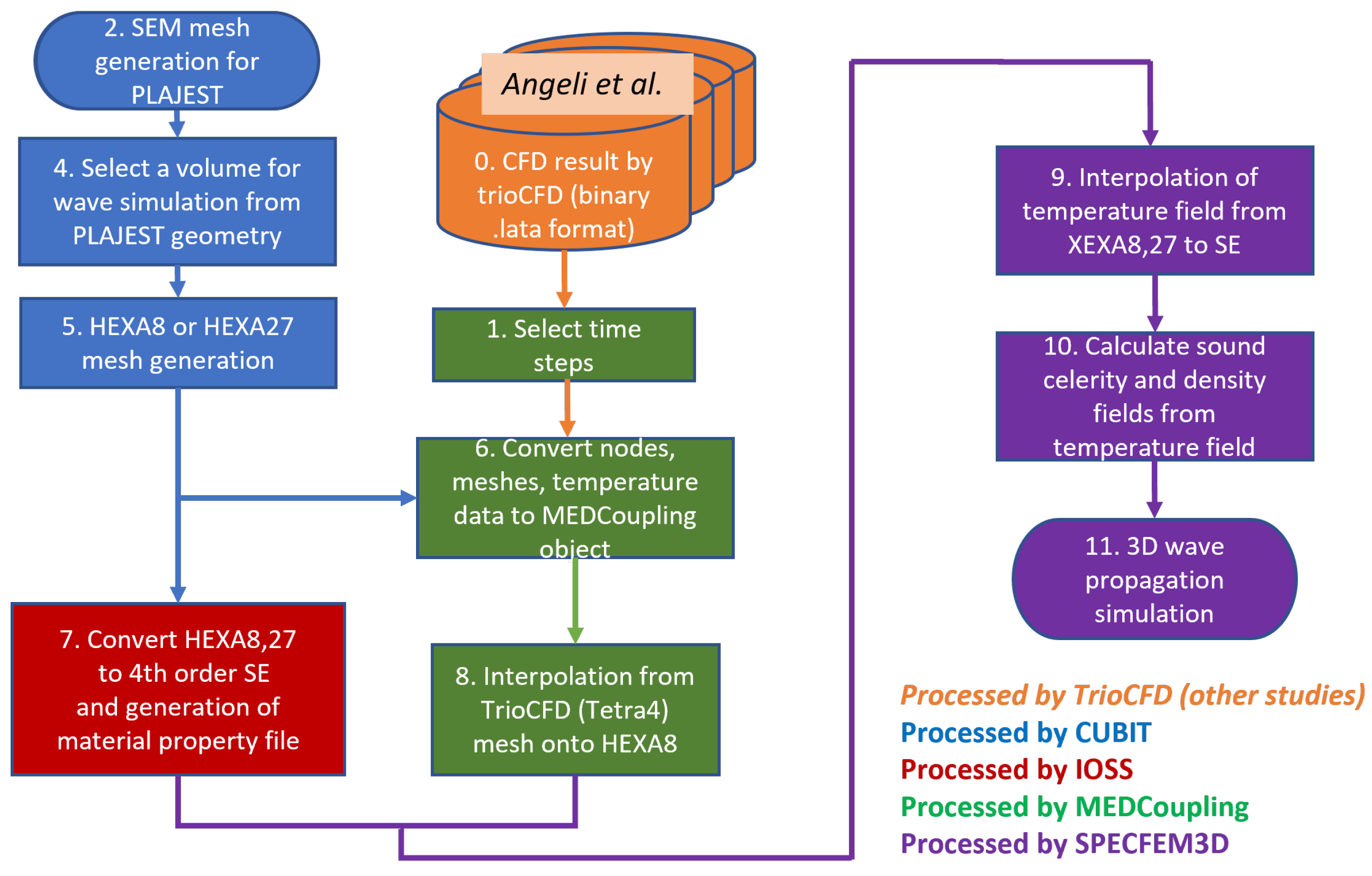
This thermal–hydraulic data obtained from a calculation with the CFD code “TrioCFD” was used to completely describe the medium in which ultrasounds propagate. The type of finite element of the meshes used in the two codes TrioCFD and SPECFEM3D is not the same, so we needed to perform preprocessing to import the result of CFD into our acoustic simulation. Figure 4 shows the entire workflow of this process.

Tetrahedral elements with four nodes were used in the CFD calculation with TrioCFD. The total number of elements was 5,582,706, and the characteristic mesh length was set to $1.40$ $\mathrm{m}$$\mathrm{m}$. The first 200 $\mathrm{s}$ of their calculation were removed so as to obtain a good stabilization of the flow state in this CFD calculation. Thus, this calculation eventually provided us with 200–210 $\mathrm{s}$ of data of fluctuating flow status with a time step of 1 $\mathrm{m}$$\mathrm{s}$. The total number of time steps was 10,000. In the result data, temperature field values are defined at the center of each TrioCFD tetrahedral mesh element, and flow velocity values are defined on the vertex nodes. These values were to be transferred to our hexahedral mesh for SPECFEM3D. Interpolation onto each node of the SPECFEM3D hexahedral mesh was performed using the simulation data management tool called MEDCoupling. MEDCoupling is part of the pre-/postprocessing platform SALOME (https://www.salome-platform.org/downloads/current-version) and is also available as a library.

In order to prepare a mesh for SPECFEM3D calculation, we firstly selected a partial region for wave propagation simulation from the entire PLAJEST simulation model (Step 4 in Figure 4). This extraction of the domain was performed in order to eliminate acoustically uninteresting parts from the PLAJEST geometry, and this enabled us to reduce the required amount of computer memory, which is one of the limitations of wave simulations in large 3D models.

After selecting the domain, we built the first-/second-order hexahedral mesh for SPECFEM3D using the meshing software CUBIT developed by Sandia National Laboratories (USA) (Step 5).

The actual mesh type that SPECFEM3D uses is not a first- nor second-order hexahedral mesh but a fourth-order spectral element. Thus, we then performed this conversion as the final step of mesh preparation (Step 7). In order to speed up this conversion process, we used the IOSS (IO Systems) library. This library is included in the finite element analysis supporting software called SEACAS (Sandia National Laboratories).

After finishing the preparation of mesh data, the temperature field transfer was carried out, i.e., interpolation of temperature values defined at the barycentre of each tetrahedral finite element to corner nodes of the hexahedral spectral elements (Step 8) using MEDCoupling. The MEDCoupling mesh-to-node transfer function does not support HEXA27 (second-order hexahedral finite elements); consequently, if the interpolation target mesh is of the HEXA27 type, we first split HEXA27 into eight parts of the HEXA8 type (first-order hexahedral finite elements) and then use the MEDCoupling interpolation function for those HEXA8 elements.

Then, SPECFEM3D performed the interpolation of these values onto each Gauss–Lobatto–Legendre point in Step 9.

The flow velocity data were not used for our simulation, as the temperature gradient has a greater influence on the wave path than the velocity vector field [22].

To determine the element size for the mesh, we used the two conditions: the Courant–Friedrich–Lewy condition (CFL), described in Equation (7), and the number of elements per wavelength:

$$\begin{array}{c}\hfill C_p\frac{\mathsf{\Delta }t}{\mathsf{\Delta }{x}_{gll}}\le \alpha ,\end{array}$$

(7)

where $\mathsf{\Delta }t$ is the time step, and $\mathsf{\Delta }{x}_{gll}$ is the minimum interval between two GLL grid points. An averaged Courant number $\alpha$ = 0.4 was selected. and the wave celerity was defined as the highest one $C_p$ = $2416.268$ $\mathrm{m}$/${\mathrm{s}}^{-1}$. This celerity was calculated with the lowest temperature value 274.5 °C in the CFD simulation. In Equation (7), $\mathsf{\Delta }{x}_{gll}$ is not the mesh size itself; rather, it is the distance interval between GLL grid points within the spectral elements. This led us to calculate a mesh size $\mathsf{\Delta }x$ = $8.05\times {10}^{-4}$ $\mathrm{m}$ and a time step of $2.3\times {10}^{-8}$ $\mathrm{s}$. A total of 5,000 steps were simulated in order to have a sufficient total physical duration for the waves to travel through the entire simulation domain. The meshing used in the simulation thus comprises 3,250,000 spectral elements and a total number of GLL nodes of 215,320,764. This time step corresponds to a 43.5 MHz sampling frequency, which corresponds to a fine sampling for the ultrasonic simulated signal.

Figure 6 represents some examples of the preprocesses of temperature field transfer and mesh generation for SPECEFM3D. The temperature field in the tetrahedral elements of TrioCFD is indicated with transparent color on the interpolated field of the hexahedral mesh for SPECFEM3D. The image on the left side is a close-up on one of these three examples.

5. Temporal Temperature Fluctuation Measurement by Ultrasounds

The analysis of the temperature fluctuation was performed over a total duration of approximately 10 $\mathrm{s}$, from $200.000$ $\mathrm{s}$ to $210.197$ $\mathrm{s}$. Because the computation time allocated on the supercomputers that we used was limited, it was not possible to run the temperature field interpolation and wave propagation calculation processes for all of these CFD time steps. Instead, we had to extract several time steps from the temperature field with a wider time interval from the CFD results. In order to select the minimum time interval to be used for our acoustic simulation, we exploited the power spectral density (PSD) curve calculated in Figure 7 [27]. This curve allows knowing the frequency of the temperature fluctuation at x = $-0.015$ $\mathrm{m}$ (between the left and the central jets), y = $0.09$ $\mathrm{m}$ (middle point on the y axis) and z = $0.1$ $\mathrm{m}$. This is a normalized PSD calculated by dividing the original PSD with the maximum PSD value. The peak of this PSD curve is found around 3 $\mathrm{Hz}$ and is in accordance with experimental results, as mentioned by Angeli in [27]. This peak is lower than 5 $\mathrm{Hz}$. This peak is followed by a slope (Kolmogorov slope).

In this work, all our simulations were performed on two of the largest supercomputers in Europe: CURIE (CEA TGCC) and OCCIGEN (CINES), both part of Grand Équipement National de Calcul Intensif (GENCI). Despite the use of these supercomputers, we knew that it would be difficult to perform calculations with a fine temporal step. In order to be able to follow the fluid dynamics, we wanted to confirm fluid fluctuations at a 3 $\mathrm{Hz}$ frequency as seen in PSD curves. We fixed the frequency limit to 5 $\mathrm{Hz}$, then the Shannon sampling criterion imposed us to use a minimum sampling frequency of 10 $\mathrm{Hz}$). Temperature fields were thus extracted from the complete volume with a $0.1$ $\mathrm{s}$ interval.

The computation domain was divided into 256 parts, and parallel calculations were carried out. The duration of the interpolation of a temperature field from a TrioCFD result to SPECFEM3D was approximately 20 h using a single CPU at one chosen altitude and one time step (the insonified area represented in Figure 2). The average duration for an acoustic simulation was about 26 min, excluding the mesh generation and the interpolation processes of the temperature fields, which were performed once and for all. Complete results, signals at each point in the volume, cannot be fully stored on a physical disc because of the high number of calculations. Thus the data resulting from SPECFEM3D calculations were recorded for several planes, as described in Figure 3.

To analyze temporal temperature fluctuations within our heterogeneous medium and then to make the correlation with ultrasonic data, a PSD curve was calculated at three different points. These three points have the same y and z position (y = $0.09$ $\mathrm{m}$ and z = $0.1$ $\mathrm{m}$) and a different x position (x = −0.035 m, 0.0 m and 0.035$\mathrm{m}$). The position y = $0.09$ $\mathrm{m}$ corresponds to the middle of the jets along the y axis, and z = $0.1$ $\mathrm{m}$ corresponds to an altitude with high turbulence. x = $0.0$ $\mathrm{m}$ is in the middle of the central jet. x = −0.035 m and 0.035$\mathrm{m}$ are two positions between the cold jet and the hot jet. These values are imposed by the initial choice of recorded planes (Figure 3). In these positions, temperature fluctuations are high but probably less than for positions x = −0.015 m and 0.015$\mathrm{m}$ chosen by Angeli et al. Figure 8A,B shows the temperature PSD curve of the original CFD results (every millisecond) at three selected points and the same kind of curves but with only extracted time steps (every $0.1$ $\mathrm{s}$), respectively.

Using the finer sampling, the peak of the experimental PSD curve is confirmed at 3 $\mathrm{Hz}$ for each position. Using data with a coarser time step gives merely the same results for the central point, as the peak frequency at 3 $\mathrm{Hz}$ is clearly visible. From these comparisons, we thus verify that the peak frequency of the temperature fluctuation is possibly detected. In the next step, the idea is to search for this flow indicator using ultrasonic measurements. The ultrasonic parameters which are selected are the maximum amplitude of the wave at one point and the corresponding time of flight (TOF). Two examples are shown in Figure 9. The two points have the same altitude: one point is close to the jet, and the second one is after the three jets (from the emitter position). The position x = $0.035$ $\mathrm{m}$ is close to the jets, and the temperature behavior exhibits clear periodic fluctuation. The position x = $0.105$ $\mathrm{m}$ is far from the jets, and the temperature remains constant over the 10 $\mathrm{s}$ of the CFD simulation, so the corresponding PSD curve gives no frequency information. At the position x = $0.035$ $\mathrm{m}$, among the two PSD calculated with ultrasonic parameters, only those calculated with the time of flight exhibit a clear 3 $\mathrm{Hz}$ peak as for the temperature PSD. At the position x = $0.105$ $\mathrm{m}$, the same observation is performed: the time-of-flight PSD exhibits a clear 3 $\mathrm{Hz}$ peak as for the temperature PSD. This result is very interesting, as it demonstrates that the history of temperature fluctuations is transported by the ultrasonic wave and a receiver positioned after the jets is able to analyze the temperature fluctuation.

The idea is further deepened using measurements of time-of-flight PSDs at various positions along the x-axis. These curves are compared with PSD curves calculated on CFD data. The resulting curves are presented in Figure 10.

The calculation of the PSDs with the low sampling CFD data (sampling frequency of 10 $\mathrm{Hz}$) shows that only the PSDs on the positions x = −0.035 m and 0.035 $\mathrm{m}$ exhibit a frequency peak at 3 $\mathrm{Hz}$. On the other hand, as expected, following the hypothesis of the transport of the fluctuation information by the ultrasonic wave, for positions beyond x = $-0.035$ $\mathrm{m}$, all the time-of-flight PSDs contain this information. We also cumulated (added) all the PSDs calculated at the different points, the PSD curve being defined as a cumulated temperature PSD curve in Figure 10. The 3 $\mathrm{Hz}$ peak emerges clearly with a secondary peak at 1 $\mathrm{Hz}$. The comparison with the PSD of the TOF at x = $0.105$ $\mathrm{m}$ shows that the ultrasonic measurement clearly indicates this peak but does not find the secondary peak. There is therefore a limit in the sensitivity of the detection of these fluctuations by an ultrasonic measurement technique, but simulations and results demonstrate that a pair of transducers positioned in a through-transmission setup would allow the temperature fluctuation frequency to be registered.

6. Conclusions

We designed an extensive physical and numerical simulation strategy to study the potential of ultrasonic measurements to monitor turbulent flow. The study was focused on liquid metal flows for which ultrasonic measurements are the best candidate to monitor flows. In the case of sodium flow monitoring inside SFR nuclear reactors, it is planned that transducers will be positioned in the flows. There are not many experiments being conducted on liquid sodium flows, as they are still very difficult to perform, and there are not many SFR nuclear reactors in operation worldwide.

One of the main difficulties, when trying to assess measurement performance without using real experiments, lies in simulating ultrasonic propagation in a representative flow. Our simulation strategy consisted of selecting a high-level CFD simulation of a real experiment of liquid metal jet mixing. We also drew on previous studies concerning ultrasonic wave propagation in liquid sodium to define all physical parameters for the wave simulation. The novelty of this study consisted in making a wave propagation simulation for several CFD time steps to validate the potential of ultrasonic measurements to follow flow fluctuations. Our analysis of flow fluctuation enabled us to prove that the frozen-flow hypothesis was completely valid in this study. It should be underlined that such a hypothesis is rarely numerically studied. The study required the development of dedicated tools to implement the wave propagation modeling on high-performance computers. The SPECFEM3D code was chosen as the numerical calculation tool for its numerical efficiency because of matured development for massively parallelized computing on HPCs and the application of the spectral-element method.

Despite significant computer resources, we had to limit the maximum frequency observed to 5 Hz in order to be able to complete the study. This limit was enough to demonstrate that the main flow fluctuation frequency of 3 Hz can be monitored using a pair of transducers in a through-transmission setup. This demonstration opens the way for developing more simulations combining CFD simulations and wave propagation for several time steps so that better ways to monitor fluctuating flows could be developed. One limitation of these studies is the huge volume of data to be stored to study wave propagation in detail. This volume could be drastically reduced when transducer positions are not a parameter of investigation. The advantage of a pair of transducers is that it makes it possible to monitor flow between the two transducers. The wave propagates from the emitter in the flow and, to some extent, transfers the flow history to the receiver.

In this study, the flow history is the fluctuation of the flow temperature. This study proves that it is now possible to conduct simulations of wave propagation in a more realistic flow geometry. There is of course still a step to be taken to be able to conduct simulations in large and long flows.