Quantitative Inspection of Complex-Shaped Parts Based on Ice-Coupled Ultrasonic Full Waveform Inversion Technology

Featured Application

Nondestructive testing and structural health monitoring for complex-shaped parts with a high resolution.

Abstract

Ultrasonic methods have been extensively developed in nondestructive testing for various materials and components. However, accurately extracting quantitative information about defects still remains challenging, especially for complex structures. Although the immersion technique is commonly used for complex-shaped parts, the large mismatch of acoustic impedance between water and metal prevents effective ultrasonic transmission and leads to a low signal-to-noise ratio(SNR). In this paper, a quantitative imaging method is proposed for complex-shaped parts based on an ice-coupled full waveform inversion (FWI) method. Numerical experiments were carried out to quantitatively inspect the various defects in a turbine blade. Firstly, the k-space pseudospectral method was applied to simulate ice-coupled ultrasonic testing for the turbine blade. The recorded full wavefields were then applied for a frequency-domain FWI based on the Limited-memory Broyden–Fletcher–Goldfarb–Shanno (L-BFGS) method. With a carefully selected iterative number and frequency, a successive-frequency FWI can well detect half wavelength defects. Extended studies on an open notch with different orientations and multiple adjacent defects proved its capability to detect different types of defects. Finally, an uncertainty analysis was conducted with inaccurate initial velocity models with a relative error of ±2%, demonstrating its robustness even with a certain inaccuracy. This study demonstrates that the proposed method has a high potential to inspect complex-shaped structures with an excellent resolution.

1. Introduction

Rapid development in the fields of computer technology, manufacturing techniques and materials science makes the geometry of key components more complex. For example, instead of an assembly of a disk and removable blades, the integratedbladed disk (BLISK) technology has been widely applied in the aeroengine design due to the merits of a light weight, high aerodynamic efficiency, excellent fatigue resistance and high efficiency of fuel consumption [1]. Recently, such monocoque components have been conveniently designed and fabricated by the emerging additive manufacturing (AM), also known as 3D printing technology. Although AM has an excellent ability to manufacture complex-shaped parts with an optimal structure design, the quality of manufactured products may be influenced by buckling, residual stress and internal defects during the cooling process [2]. Moreover, there is a higher tendency to bring in defects in complex-shaped parts due to a much greater surface area. Therefore, to guarantee the safety of these key components, special attention should be paid to the quantitative nondestructive testing (NDT) of complex-shaped parts. X-ray computed tomography (XCT) is widely used to inspect such parts in an industrial application. Although XCT possesses a high sensitivity to volumetric defects such as gas pores and inclusions, it is insensitive to planar defects such as cracks and delamination [3]. In addition, a high energy X-ray source is required for thick metals, resulting in radiation hazards and expensive equipment.

On the other hand, ultrasound plays an irreplaceable role in NDT with the advantages of a large penetration depth, large area coverage and high sensitivity to both internal and surface defects. Both a single transducer with a scanning system and a transducer array have been widely applied to develop methods to visualize ultrasonic results with various imaging algorithms. Synthetic imaging methods including a common source method (CSM) [4,5], a synthetic aperture focusing technique (SAFT) and a total focusing method (TFM) [6,7] have been well developed to produce high resolution images for the objects below the measurement based on the wave reflections. However, when the surface of the tested object is uneven or irregular, the deployment of contact transducers will be difficult and poor coupling will lead to inaccurate or false detection. Currently, there are three common schemes to tackle this issue. The first method is to integrate the transducer with a wedge or “shoe” to match the surface to allow direct contact. This method is indeed simple but a wedge is only suitable for one specific surface. When the surface profile is varying or too complex, this method is difficult or even impossible to apply. The second method is to use flexible transducers [8], which show a greater compatibility than wedges. However, a few potential defects may go undetected in the dead zone because of the near field. The third method is to place the tested object into a water-filled chamber and the water acts as an acoustic couplant [9]. As a whole water-filled regular structure, objects with highly curved surfaces can be inspected. However, there is a large difference of acoustic impedance between the water and metal materials that hinders ultrasonic energy from effectively penetrating into the tested metal object. Thus, the performance is limited for metal parts with complex shapes.

Recently, to bridge the gap between the immersion method and the contact method, Simonetti et al. proposed a cryo-ultrasonic method to inspect complex-shaped parts, which were encased in ice with a cylinder container [10]. As the longitudinal wave speed of ice is about 2.5 times that of water, the acoustic impedance mismatch with the metal material can be greatly reduced so that the transmission energy will significantly increase. Their preliminary results demonstrated its superiority compared with the immersion method. Furthermore, they presented experimental schemes to avoid the formation of crack and bubble nucleation when water is freezing [11]. To reconstruct the internal complex structure of such an ice-encased part, traditional focusing imaging methods are no longer suitable. Focusing imaging can precisely localize the defects but it is difficult to obtain the information of the shape and appearance. Moreover, these methods ignore multiple reflection signals and are unable to obtain the information of lower and side surfaces. Simonetti et al. applied a diffraction mitigation technique to carry out ultrasonic imaging/tomography [10,11]. However, the performance of diffraction tomography is limited due to its assumption of the first-order diffraction. It can achieve a better resolution than ray tomography but it is only suitable for low-contrast defects. Therefore, to quantitatively evaluate real defects with arbitrary forms in complex-shaped structures, a full wavefield containing all of the possible linear and higher-order diffraction effects should be considered in the tomography.

To solve the inversion problem with a recorded full wavefield, full waveform inversion (FWI) tomography was firstly derived in geophysics for seismic wave imaging [12,13,14,15]. The FWI is performed via an iterative minimization of the misfit between an experimentally measured wavefield and a numerically calculated wavefield generated with a forward model. Based on a certain optimization algorithm, the estimated model of the tested object is iteratively updated. The iteration process will end when the convergence criterion is satisfied; then, the final model is the approximation of the tested object. FWI automatically considers higher-order scattering effects; thus, it has been widely studied in medical applications for breast cancer screening and diagnosis [16], bone quantitative imaging [17] and delamination detection in civil infrastructures [18,19]. Recently, FWI has also been applied in guided wave technology to quantify corrosion defects in plate-like structures [20,21]. In this article, a frequency-domain FWI is introduced as an imaging algorithm for the quantitative defect detection in a complex structure combined with ice-coupled ultrasonic testing.

The rest of this paper is structured as follows. In Section 2, the fundamental theory of FWI including forward modelling and the successive-frequency FWI procedure will be briefly introduced. The numerical experiment setup and data calibration of the ice-coupled ultrasonic testing for turbine blades are then illustrated in Section 3. The reconstructed results for various defects are shown and discussed in Section 4. Finally, concluding remarks are drawn in Section 5.

2. Theory of Full Waveform Inversion

A detailed description of the FWI algorithm can be found in the literature [13,15]; thus, only the key techniques and steps are briefly introduced here. Generally, FWI imaging can be regarded as a composition of three segments: forward modeling to generate calculated data by solving a wave equation, the computation of the gradient and Hessian matrix of the misfit function and updating the model with a suitable optimization method.

2.1. Forward Modelling for Ultrasonic Wave Propagation

Reliable forward modelling for wave propagation is a primary prerequisite for ultrasonic FWI tomography. Ultrasonic wave propagation in solids is typically described by an elastic wave equation [22]. To boost the whole efficiency of FWI, the scalar acoustic wave equation is usually used to approximate the ultrasonic wave propagation [17]. The formalism of a 2D acoustic wave equation in a frequency-domain is expressed as:

$$({\nabla }^2+{\omega }^2{m}^2)\psi (r,\omega )=-s(r,\omega )$$

(1)

where ${\nabla }^2=\frac{{\partial }^2}{\partial x^2}+\frac{{\partial }^2}{\partial z^2}={\partial }_x^2+{\partial }_z^2$ is the Laplace operator, $\omega$ is the angular frequency, $m=1/c$ is the slowness, $c$ is the wave speed, $r=(x,z)$ is the spatial position in the Cartesian coordinate system and $\psi (r,\omega )$ is the displacement wavefield. $s(r,\omega )=s(\omega )\delta (r-r_s)$ is the excitation signal where $s(\omega )$ refers to the Fourier transform of the source, $\delta (r-r_s)$ denotes the Dirac function and $r_s$ is the excitation position.

The finite difference technique is the most common method to solve partial differential equations [23,24] and is applied in forward modelling here. In order to simplify the denotation, Equation (1) can be expressed by the matrix equation $\mathbf{F}\mathsf{\psi }=\mathbf{s}$, where $\mathbf{F}={\nabla }^2+{\omega }^2{m}^2$ is a $l\times l$ complex-valued impedance matrix, which is related to the frequency, material properties, discrete format and boundary conditions. $\mathsf{\psi }$ and $\mathbf{s}$ are $l\times 1$ column vectors at the nodal points of the discrete grid.

To reduce the computation cost, the LU factorization is utilized to solve the wavefield $\mathsf{\psi }$:

$$LU\mathsf{\psi }=\mathbf{s}$$

(2)

where $\mathbf{L}$ and $\mathbf{U}$ denote the lower and upper triangular matrices from the LU factorization. As the solution is reusable for different sources to solve the forward problem, multiple source problems can be handled efficiently [25]. To alleviate the computation burden and avoid reflection interference, a perfectly matched layer (PML) boundary condition is applied around the computational domain to absorb outgoing waves in a similar configuration as done in [26].

2.2. Full Waveform Inversion

The aim of inversion is to find a model parameter $\mathbf{m}=[m_1,m_2,\dots ,m_{n_x{n}_z}{]}^t$ in the model space to reduce the residual between the calculated and measured data. A least-square norm is chosen to define this misfit as the object function:

$$\underset{m}{\min }E(\mathbf{m})=\frac{1}{2}\parallel P_r(\mathsf{\psi })-\mathbf{d}{\parallel }^2=\frac{1}{2}(\Delta {\mathbf{d}}^t)\ast \Delta \mathbf{d}$$

(3)

where $P_r$ is the sampling operator to extract the wavefield at the receivers from the forward model. $\mathsf{\psi }=\left\{{\psi }_i\right\}, i=(1,2,\dots ,n_r)$ and $\mathbf{d}=\left\{d_i\right\}, i=(1,2,\dots ,n_r)$ are the calculated and measured data vectors, respectively. $\Delta \mathbf{d}=\{P_r({\psi }_i)-d_i\}, i=(1,2,\dots ,n_r)$ is the residual vector. The superscript $t$ is the vector or matrix transposed and $\ast$ is the complex conjugate to convert the object function to real numbers.

Various optimization algorithms can be applied to minimize the object function $E(\mathbf{m})$. First and foremost, the gradient of $E(\mathbf{m})$ should be defined with respect to the model parameters such as density, wave speed and attenuation. It offers the direction to iteratively update the vector space to minimize the misfit [27]. Based on Taylor’s theorem, we have:

$$E(\mathbf{m}+\delta \mathbf{m})\approx E(\mathbf{m})+\mathbf{g}\cdot \delta \mathbf{m}+\frac{1}{2}\delta {\mathbf{m}}^t\cdot \mathbf{H}\cdot \delta \mathbf{m}=P(\delta \mathbf{m})$$

(4)

where $\mathbf{g}=\frac{\partial E(\mathbf{m})}{\partial \mathbf{m}}=\Re e({\mathbf{J}}^t\Delta {\mathbf{d}}^{\ast })$ is the gradient with a size of $l\times 1$. $\mathbf{J}=[\frac{\partial {\psi }_p(m_q)}{\partial m_q}], p=(1,2,\dots ,n_r);q=(1,2,\dots ,n_x{n}_z)$ is the $n_r\times l$ order Fréchet derivative matrix and $\Re e$ denotes the real part of the complex value. $\mathbf{H}=\frac{{\partial }^{2}E(\mathbf{m})}{\partial {\mathbf{m}}^2}$ is the Hessian matrix. To minimize the object function $E(\mathbf{m})$, let $\frac{dP(\delta \mathbf{m})}{d(\delta \mathbf{m})}=\mathbf{g}+\mathbf{H}\delta \mathbf{m}$ be zero then $\delta \mathbf{m}=-{\mathbf{H}}^{-1}\cdot \mathbf{g}$. Therefore, the model can be updated as:

$${\mathbf{m}}_{k+1}={\mathbf{m}}_k-\epsilon {\mathbf{H}}^{-1}\mathbf{g}$$

(5)

where $\epsilon$ is the step length. When only the first-order derivative is considered, the corresponding method is called the steepest descent method. It is a straightforward way, but its convergence rate is so slow that it limits the application for large-scale problems [17]. To boost the convergence, the second-order derivative should be taken into consideration. However, the computation amount and storage space increase sharply because of the calculation of the inverse Hessian matrix ${\mathbf{H}}^{-1}$. To handle this problem, quasi-Newton methods have been developed to approximate the Hessian matrix. The limited-memory Broyden–Fletcher–Goldfarb–Shanno (L-BFGS) method is one of the most popular methods. This method calculates the approximation of the inverse Hessian matrix by a limited number ($n_{lim}$) of the gradient-difference and model-difference vectors associated with the $n_{lim}$ latest iteration ($n_{lim}$ is generally defined between 3 and 20) [28].

At every iteration ${\widehat{n}}_{lim}=\min \{n_{lilm},k-1\}$, correction pairs $\{{\mathsf{\alpha }}_i,{\mathsf{\beta }}_i\},i=k-{\widehat{n}}_{lim},k-{\widehat{n}}_{lim}+1,\dots ,k-1$ are stored, where ${\mathsf{\alpha }}_i={\mathbf{m}}_{i+1}-{\mathbf{m}}_i$, ${\mathsf{\beta }}_i={\mathbf{g}}_{i+1}-{\mathbf{g}}_i$. Let ${\mathsf{\gamma }}_i=\frac{1}{{\mathsf{\beta }}_i^t{\mathsf{\alpha }}_i}$, ${\mathsf{\eta }}_i=(\mathbf{I}-{\mathsf{\gamma }}_i{\mathsf{\beta }}_i{\mathsf{\alpha }}_i^t)$, $\mathbf{B}={\mathbf{H}}^{-1}$, if $k+1<=l$, then

$$\begin{array}{l}{\mathbf{B}}_k={\mathsf{\eta }}_{k-1}{}^t{\mathbf{B}}_{k-1}{\mathsf{\eta }}_{k-1}+{\mathsf{\gamma }}_{k-1}{\mathsf{\alpha }}_{k-1}{\mathsf{\alpha }}_{k-1}{}^t\\ {=\mathsf{\eta }}_{k-1}^t{\mathsf{\eta }}_{k-2}^t\dots {\mathsf{\eta }}_0^t{\mathbf{B}}_k^0{\mathsf{\eta }}_0\dots {\mathsf{\eta }}_{k-2}{\mathsf{\eta }}_{k-1}+{\mathsf{\eta }}_{k-1}^t{\mathsf{\eta }}_{k-2}^t\dots {\mathsf{\eta }}_1^t{\mathsf{\gamma }}_0{\mathsf{\alpha }}_0{\mathsf{\alpha }}_0^t{\mathsf{\eta }}_1\dots {\mathsf{\eta }}_{k-2}{\mathsf{\eta }}_{k-1}+\dots +{\mathsf{\eta }}_{k-1}^t{\mathsf{\gamma }}_{k-2}{\mathsf{\alpha }}_{k-2}{\mathsf{\alpha }}_{k-2}^t{\mathsf{\eta }}_{k-1}+{\mathsf{\gamma }}_{k-1}{\mathsf{\alpha }}_{k-1}{\mathsf{\alpha }}_{k-1}^t\end{array}$$

(6)

If $k+1>l$, the iterative expression is given by:

$$\begin{array}{l}{\mathbf{B}}_k={\mathsf{\eta }}_{k-1}{}^t{\mathbf{B}}_{k-1}{\mathsf{\eta }}_{k-1}+{\mathsf{\gamma }}_{k-1}{\mathsf{\alpha }}_{k-1}{\mathsf{\alpha }}_{k-1}{}^t\\ {=\mathsf{\eta }}_{k-1}^t{\mathsf{\eta }}_{k-2}^t\dots {\mathsf{\eta }}_{k-l}^t{\mathbf{B}}_{{}_k}^0{\mathsf{\eta }}_{k-l}\dots {\mathsf{\eta }}_{k-2}{\mathsf{\eta }}_{k-1}+{\mathsf{\eta }}_{k-1}^t{\mathsf{\eta }}_{k-2}^t\dots {\mathsf{\eta }}_{k-l+1}^t{\mathsf{\gamma }}_{k-l}{\mathsf{\alpha }}_{k-l}{\mathsf{\alpha }}_{k-l}^t{\mathsf{\eta }}_{k-l+1}\dots {\mathsf{\eta }}_{k-2}{\mathsf{\eta }}_{k-1}\dots +{\mathsf{\eta }}_{k-1}^t{\mathsf{\gamma }}_{k-2}{\mathsf{\alpha }}_{k-2}{\mathsf{\alpha }}_{k-2}^t{\mathsf{\eta }}_{k-1}+{\mathsf{\gamma }}_{k-1}{\mathsf{\alpha }}_{k-1}{\mathsf{\alpha }}_{k-1}^t\end{array}$$

(7)

In practical cases, the initial guess of ${\mathbf{B}}_k^0$ can be computed by ${\mathbf{B}}_k^0=\frac{{\mathsf{\beta }}_k{}^t{\mathsf{\alpha }}_k}{\left|\right|{\mathsf{\beta }}_k|{|}_2^2}\mathbf{I}$, where $\mathbf{I}$ is the identity matrix [28]. With the approximation of the inverse Hessian matrix, it is easy to update the model with Equation (5). When proper convergence criteria or the maximum iteration numbers are set, the final model can be obtained as the inversion results.

The flow chart of the FWI algorithm is illustrated in Figure 1. When only one frequency is applied to the update model, no external loop is needed to perform and this method is called monochromatic inversion. In actual ultrasonic testing, the ultrasonic signal contains not just a single frequency. When several frequencies are used simultaneously during the inversion, the robustness will be improved but it comes at the cost of an increased computational time. In this case, they can be classified as a successive-frequency inversion and a simultaneous multi-frequency inversion. In this research, the successive-frequency inversion is applied, as shown in Figure 1.

3. Numerical Experiments on a Turbine Blade

To verify the feasibility and performance of the proposed ice-coupled ultrasonic FWI tomography to evaluate the defects in complex-shaped parts, a series of numerical experiments were conducted. The turbine blade is a typical safety-critical component in the aerospace industry with a complex geometry, as shown in Figure 2a. In conventional ultrasonic testing, phased array ultrasonic transducers can only be placed to directly contact smooth surfaces at the upper part. It makes the defects at the lower part difficult to inspect, such as the red circles in Figure 2a. To inspect the defects at different positions, the transducer should be moved to different positions, shown as the red line. This complex object was applied in this study. To save computational costs and storage space, only 2D tomography was carried out for a typical cross section of the turbine blade in this study, as shown in Figure 2b. To facilitate the fast acquisition of a full ultrasonic wavefield for FWI tomography, an acoustic model rather than an elastic model was adopted here to simulate the process of ice-coupled ultrasonic testing because the acoustic model is commonly employed in ultrasonic NDT research [21,29]. All of the wave phenomena including multiple reflections from the ice-steel interface and the wave-defect interaction can be revealed in such a model. It is necessary to note that in a real case shear waves could exist in a solid due to mode conversion at the interface and defects. Numerical experiments were carried out to optimize the key parameters such as the frequency selection and iteration number to quantitatively detect different types and numbers of defects in a turbine blade.

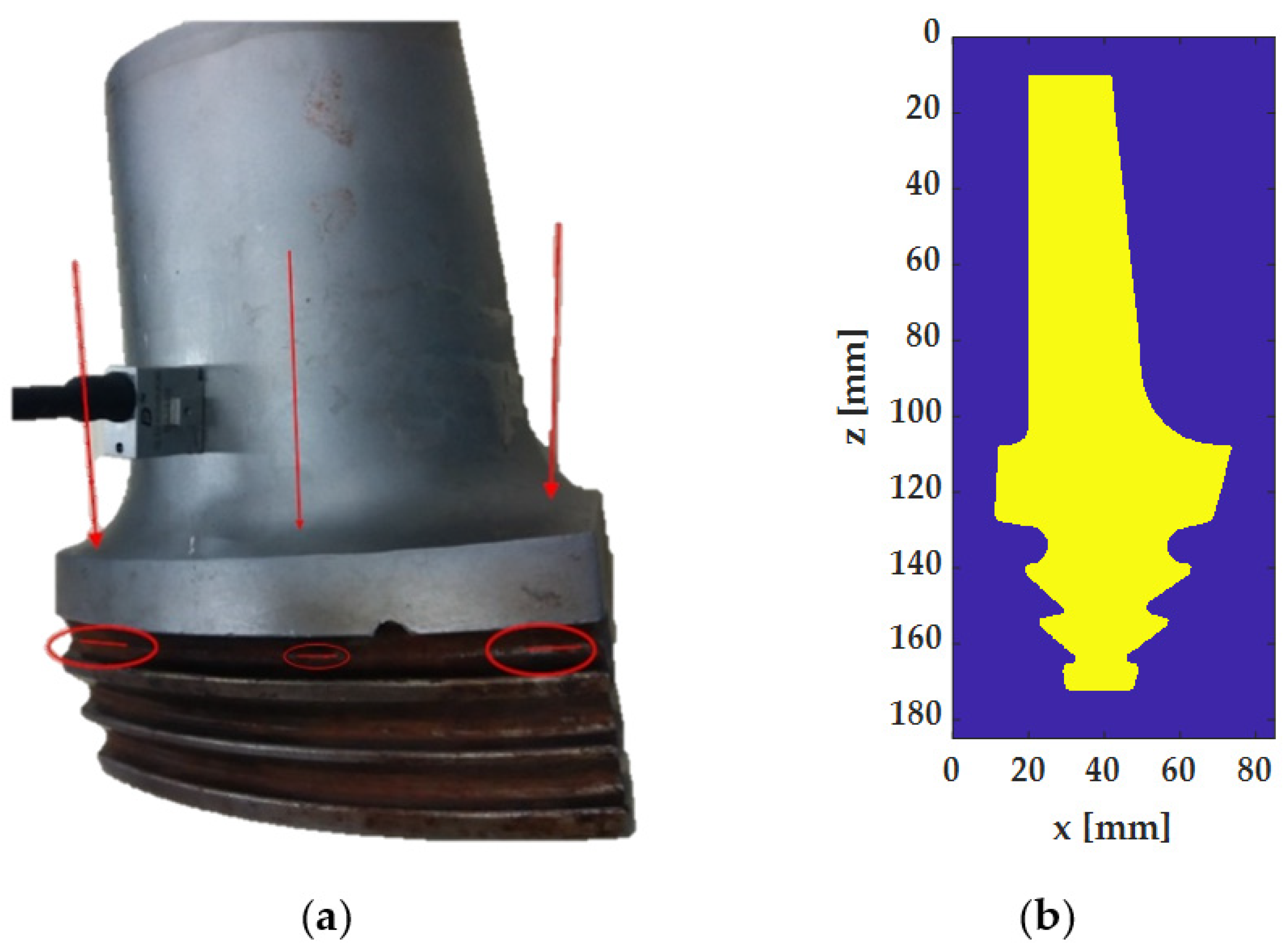
3.1. Simulation of Ice-Coupled Ultrasonic Testing in a Turbine Blade

In this study, an open-source code k-wave toolbox was applied to conduct the numerical simulation of ice-coupled ultrasonic testing to record the full wavefield [30]. This toolbox solves the acoustic wave equation based on a k-space pseudospectral method. Compared with the conventional finite difference method, the memory and computational cost were reduced dramatically.

The turbine blade was encased by ice as shown in Figure 2b. The material properties of the turbine blade and ice are shown in

Table 1. Acoustic properties of the turbine blade and ice [11].

	Mass Density ρ (kg/m3)	Wave Speed c (m/s)
Steel	7800	5875
Ice (at −5 °C)	917	4000

[11]. The size of the whole model was 185 mm × 85 mm. A series of ultrasonic transducers were deployed evenly around the turbine blade. Considering that the length of the specimen in the horizontal direction was approximately half that of the vertical direction, 6 transducers were arranged at the top and bottom sides and 12 transducers at the left and right sides, shown in Figure 3. Such an arrangement of transducers can reduce the transducer number and assure the imaging quality. At four corners, the spacing of two adjacent transducers was set as $d_1=d_2=5 \mathrm{mm}$. The PML boundary was set around the calculation domain to absorb outgoing waves and avoid reflection. To avoid uncertain factors further from the absorbing layer, all transducers were shifted inward from all sides by 1 mm. It was an effective simplification to simulate the wave propagation in a large domain because the reflections from the boundaries beyond the area of interest could be excluded by applying appropriate time gates to the recorded signals. The spacing of the transducers was $d_x=14.6 \mathrm{mm}$ in a horizontal direction and $d_z=15.73 \mathrm{mm}$ in a vertical direction.

The ultrasonic wave was excited with the following signal:

$$R(t)=[1-2{\pi }^2{f}_c^2{(t-t_0)}^2]e^{-{\pi }^2{f}_c^2(t-t_0{)}^2}$$

(8)

where $f_c$ was the center frequency and $t_0$ referred to the time delay. As the theoretical resolution of the FWI is a half wavelength [20,21], an ultrasonic wave with a center frequency of 1 MHz was applied to inspect a defect as small as 3 mm in the turbine blade. When $f_c=1\mathrm{MHz}$ and $t_0=1.5/f_c$, this excitation waveform and the corresponding amplitude spectrum are depicted in Figure 4. It could be seen that the dominant energy (above the value of a −6 dB drop from the maximum amplitude) was within the effective frequency band of 0.48 MHz–1.6 MHz. A quadrilateral mesh was applied to discretize the spatial domain and the mesh size was carefully chosen to satisfy the Courant–Friedrichs–Lewy (CFL) condition. The mesh size was chosen as $L_{element}=0.2 \mathrm{mm}$ in both directions for an accurate acoustic wave calculation up to a frequency of 2 MHz (about 10 elements per minimum wavelength) [31]. To ensure numerical stability, the time step should be chosen carefully according to the smallest element and the wave speed. Here, time step was set as $\Delta t=0.5L_{element}/c_{max}$, where $c_{max}$ was the wave speed in the steel.

The resolution and sensitivity of tomography strongly depend upon ‘ray density’ [32]. For this reason, a full matrix capture (FMC) technique was adopted to perform the ultrasonic data acquisition, which collected complete datasets including all transmitter-receiver combinations. Therefore, each transducer was excited successively and all transducers recorded the ultrasonic signals simultaneously. Finally, the resulting wavefield consisted of $N_{rec}\times N_{src}=1296$ waveforms. In a k-wave simulation, a series of $N_{src}=36$ simulations should be performed independently to obtain this full wavefield. These calculations could be practically and conveniently distributed via the different processors of a cluster. Thus, a parallelization scheme was adopted to accelerate the simulation. The sampling frequency was set to be approximately 60 MHz to satisfy the Nyquist theorem. The total time in the simulation was set as $110 \mathsf{\mu }\mathrm{s}$ to guarantee that the receiver at one corner could receive the reflected signal from the opposite corner.

3.2. Data Calibration

As the inversion procedure was performed in the frequency-domain, the recorded full wavefield should be transformed into the frequency-domain by utilizing a fast Fourier transform (FFT). It should be noted that all full waveform datasets were transformed directly and there was no need to identify and truncate direct waves collected by the receivers.

To obtain an accurate inversion result, the frequency components of the observed or recorded data must match those of the calculated data from the forward model. There was some inevitable deviation of the amplitude and phase spectrum between the recorded data and the calculated data. This deviation may bring a few errors into the inversion procedure. Therefore, a prior data calibration should be performed to match the recorded data and calculated data with an intact specimen. The correction factors for amplitude and phase were defined as [21]:

$$Q_{amp}=\frac{abs(fft({\mathsf{\psi }}_0))}{abs(fft({\mathbf{d}}_{obs,0}))}$$

(9)

and:

$$Q_{pha}=\arg (fft({\mathsf{\psi }}_0))-\arg (fft({\mathbf{d}}_{obs,0}))$$

(10)

where $abs()$ represented the modulus of a complex value, $\mathrm{a}\mathrm{r}\mathrm{g}()$ denoted the phase of a complex value and $fft()$ was the fast Fourier transform. ${\mathsf{\psi }}_0$ and ${\mathbf{d}}_{obs,0}$ were the calculated and observed data for the intact specimen. With these two factors, the recorded amplitude and phase were firstly calibrated for the following inversion process.

4. Results and Discussion

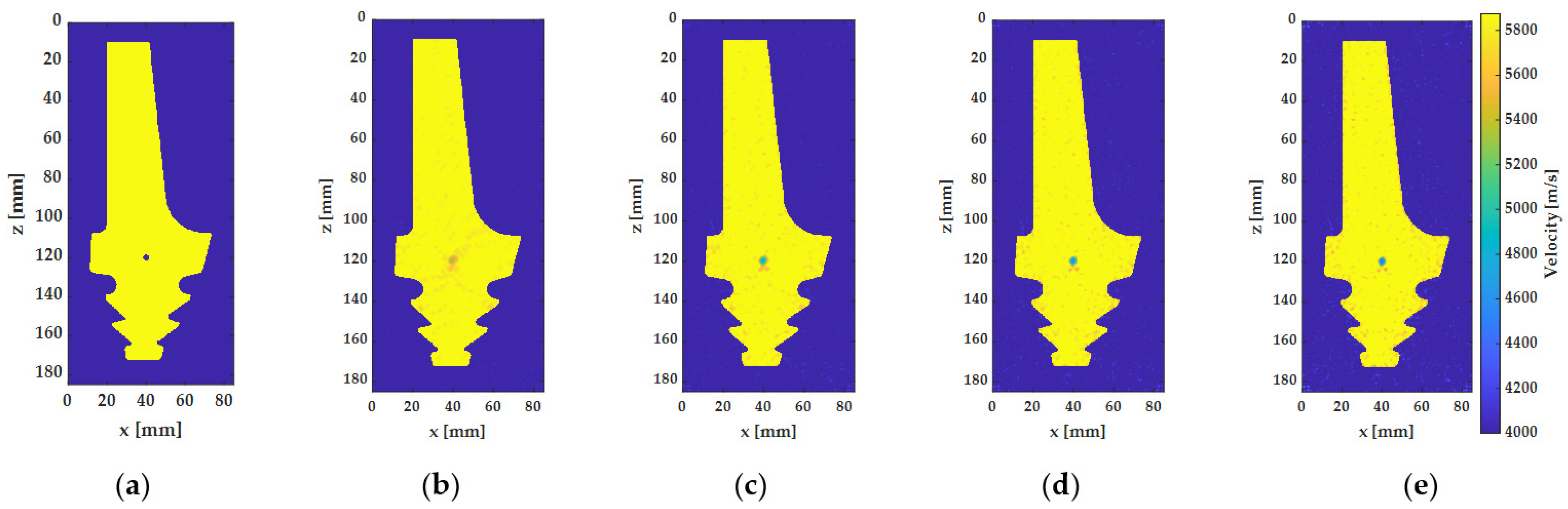
4.1. Single Internal Defect

At first, a single internal defect was embedded in a turbine blade to perform data processing and a parametric study of ultrasonic FWI tomography. For simplicity, a circular hole with a diameter of 3 mm was located at (40,120). In the first simulation, an ultrasonic wave was excited with the first transducer located at (1,6). The corresponding wave propagations at different time slots are shown in Figure 5. From the simulated wavefield, the ultrasonic wave reflected at the ice-steel interface and diffracted with the defect. At $t=6 \mathsf{\mu }\mathrm{s}$, the incident wave began to reach the edge of the blade. The reflection from the ice-steel interface can be seen in Figure 5b, indicated by a red arrow. The transmitted wave and several interface waves propagated inside the blade. When $t=21 \mathsf{\mu }\mathrm{s}$, the direct wave arrived at the receiving transducers as shown in Figure 5c. At $t=26 \mathsf{\mu }\mathrm{s}$, the propagating waves interacted with the defect, generating diffracted waves, which can be seen in Figure 5d. Finally, the ultrasonic wavefield was recorded by all of the 36 transducers. Without a loss of generality, the waveform recorded by the ${19}^{\mathrm{th}}$ receiver placed at (84,6) and its normalized amplitude spectrum are shown in Figure 6. The first wave package was the direct wave from the $1^{\mathrm{st}}$ transducer to the ${19}^{\mathrm{th}}$ transducer. In addition, there were two more waves due to the reflection at the boundary and the diffraction from the internal defects. The path of the diffraction wave from the defect is depicted in Figure 5d with blue dashed lines. The corresponding time-of-flight was about $26 \mathsf{\mu }\mathrm{s}$. Thus, the second wave package was the diffracted wave from the defect, followed by multiple waves reflected from the lower boundary of the blade. All of the reflections from the ice-steel interface and the diffraction signal from the defect can be seen in the A-scan signal in Figure 6a. Due to the complex geometry of the turbine blade, reflection signals from the boundaries were complicated and the energy was very high, making the diffracted wave from the internal defect difficult to identify. Moreover, compared with the excitation, the amplitude spectrum was distorted to a certain degree due to the existence of wave scattering phenomena, as shown in Figure 6b. Nevertheless, the recorded signal still contained information at frequencies around 1 MHz with a large bandwidth.

The number of iterations is one of the key parameters in the inversion process. With the increase of iterations, the accuracy of the inversion result will be improved but the computing time will increase linearly. Therefore, it is important to determine the number of iterations to balance the accuracy and the computation cost. The variation of the misfit function, as described by Equation (3), as a function of iterations is given in Figure 7. Obviously, the misfit monotonically decreases as the iterative number increases. After 20 iterations, the misfit was small enough (lower than 1%), indicating that the accuracy of the inversion result was high enough. The FWI tomographs for the different iterations are also shown in Figure 8. When the iteration was set to as few as k = 5, the quality of the FWI image was poor and the defect was difficult to observe. After 10 iterations, the defect became clearly visible but the detailed information of the reconstructed defect changed. When the number of iterations was larger than 20, the inversion results became stable. Hence, the number of iterations was set as 20 for the following studies. Although the inversion result converged after 20 iterations, there was still a remarkable noise in the final result.

To improve the overall accuracy of the inversion, information of different frequencies should be taken into consideration. A lower frequency has a better tolerance for a relatively large-scale structure while a higher frequency should be considered for a small substructure [15]. Therefore, successive inversions with a moving frequency from low to high were applied to mitigate the nonlinearity of the inversion problem, resulting in a more robust result than a monochromatic inversion. In this study, a frequency group of seven discrete frequencies from 400 kHz to 1600 kHz were adopted because the excited and received signals showed an effective bandwidth of 480 kHz−1600 kHz, as shown in Figure 6b. Figure 9 shows the reconstructed tomographs when the inversion finished at frequencies of 0.4 MHz, 0.6 MHz, 0.8 MHz, 1 MHz, 1.2 MHz, 1.4 MHz and 1.6 MHz, respectively. Compared with the monochromatic inversion of 1 MHz, the overall noise was reduced based on the successive inversion of low frequencies. It could be seen that with the increase of the frequency of successive inversions, the accuracy of the 3 mm diameter circular hole was improved. The cross sections through the defect along the horizontal and vertical direction are presented in Figure 10. The FWI results showed a good agreement with the profile of the true defect in both directions. To quantitatively evaluate the reconstruction accuracy, the relative error of the full width at half maximum (FWHM) along the two directions along with their root mean square (RMS) error were considered. Therefore, the three indicators were defined as $E_V=\frac{FWH{M}_V}{D_{def}}$, $E_H=\frac{FWH{M}_H}{D_{def}}$ and $E_{RMS}=\sqrt{\frac{E_V^2+E_H^2}{2}}$, where $D_{def}$ denoted the diameter of the circular defect. Figure 11 shows the variations of the relative errors of the FWHM and their RMS error as a function of the successive-frequency inversions for circular holes with different diameters. Generally, the errors decreased as the successive-frequency increased and almost converged after the frequency of 1 MHz. It meant that successive-frequency inversion could indeed improve the accuracy of FWI tomography. Especially for the 3 mm diameter defect, the relative errors sharply decreased from 28.3% to 8.5%. When the defects were larger than 3 mm, the relative errors decreased to smaller than 2%. The relatively large error for the 3 mm diameter defect was due to the fact that 3 mm is close to half of the interrogating wavelength at 1 MHz, which is the theoretical resolution of the FWI [22]. However, the final error was smaller than 8%, indicating that a successive-frequency FWI could obtain an accurate tomograph for internal defects and the resolution approached a half wavelength.

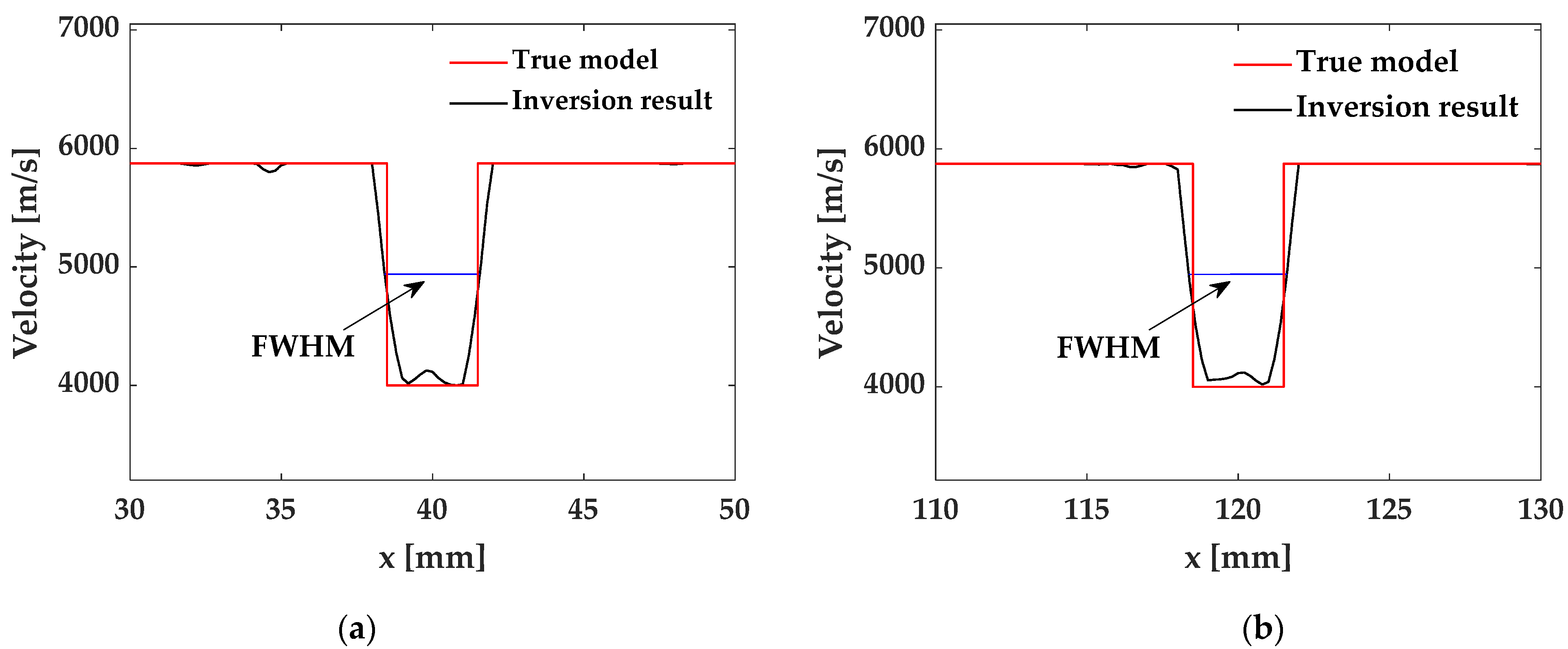
4.2. Open Notch Crack

In addition to the internal defects, a turbine blade also tends to suffer from surface cracks. Therefore, investigations were also conducted to evaluate the surface cracks based on the proposed method. Open notches with different orientations were introduced to mimic the surface crack. The size of the notch was set as a constant at 5 mm long and 2 mm wide. Only the influence of the orientation was studied and three directions ($\theta =0°,45°,90°$) were investigated here. To investigate the capability of FWI to detect open notch defects with different angles, three numerical experiments were conducted. The transducer configuration and inversion scheme remained the same as those in the previous cases. The FWI tomographs of the three notches are shown in Figure 12a,c,e. Generally, the successive-frequency FWI was able to reconstruct the surface crack with a high resolution. Similarly, to quantitatively evaluate the accuracy, relative errors defined as the profiles along the width and length were represented as $E_S$ and $E_L$. The trends of the FWHM errors with a successive-frequency are presented in Figure 12b,d,f. $E_L$ decreased significantly when the frequency was smaller than 1 MHz and converged to around 10%. However, different from the result of the circular defect in Section 4.1, $E_S$ was generally much smaller than $E_L$ and it increased with the successive-frequency. The reason might lie in the fact that ultrasound is much more capable of reconstructing the plane defects. Moreover, when the orientation of the crack was 45°, the final error was slightly higher than the other two cases. It implied that the alignment of the transducer network probably introduced some inaccuracy into the FWI results.

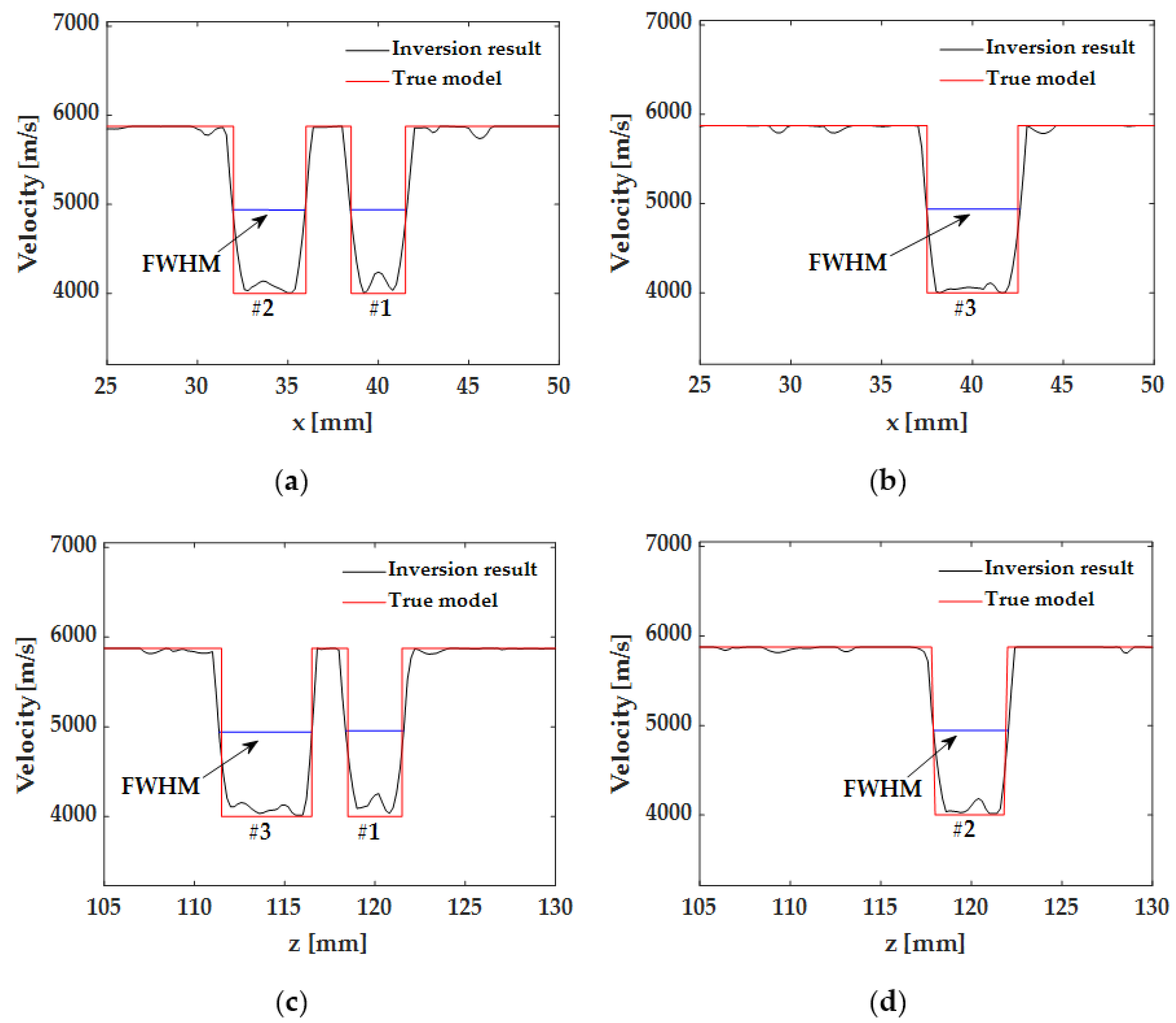
4.3. Multiple Defects

In practical engineering applications, a component probably contains multiple defects simultaneously. It should be pointed out that it is a difficult problem for an accurate inspection because multiple scattering will occur if the distance of the two defects is closed. Hence, three circular defects with different sizes were considered, as shown in Figure 13a. A central defect (marked as #1 defect) was located at (40,120) with a diameter of 3 mm. The second one with a diameter of 4 mm (marked as #2 defect) was horizontally shifted by 6 mm from #1 defect and the third one with a diameter of 5 mm (marked as #3 defect) was vertically shifted by 6 mm from #1 defect.

Similarly, a successive-frequency FWI was applied and the reconstructed defects are shown as Figure 13b. From the tomograph, these three circular defects were clearly discernable despite complex wave scattering due to the presence of the three adjacent defects. Furthermore, both vertical and horizontal profiles were compared with the true model as shown in Figure 14. The good agreement proved that the proposed method was capable of accurately detecting multiple defects in complex parts.

In addition, it is much more common that different types of defects might exist in the structure at the same time. In order to extend this study to more practical applications, an additional case study was also carried out to evaluate the structure with coexisting circular holes and cracks. Here, the circular holes were set as the same as Figure 13a and an incline notch of $45°$ was considered. The inversion results are presented in Figure 15. The FWI tomograph clearly showed the notch crack and the disperse holes. Moreover, due to the fact that the crack was relatively distant from the dispersed circular holes, the cross section profiles were very close to the results with only holes or cracks. The good agreement demonstrated that the proposed method was able to inspect different types of defects at the same time with a satisfactory accuracy.

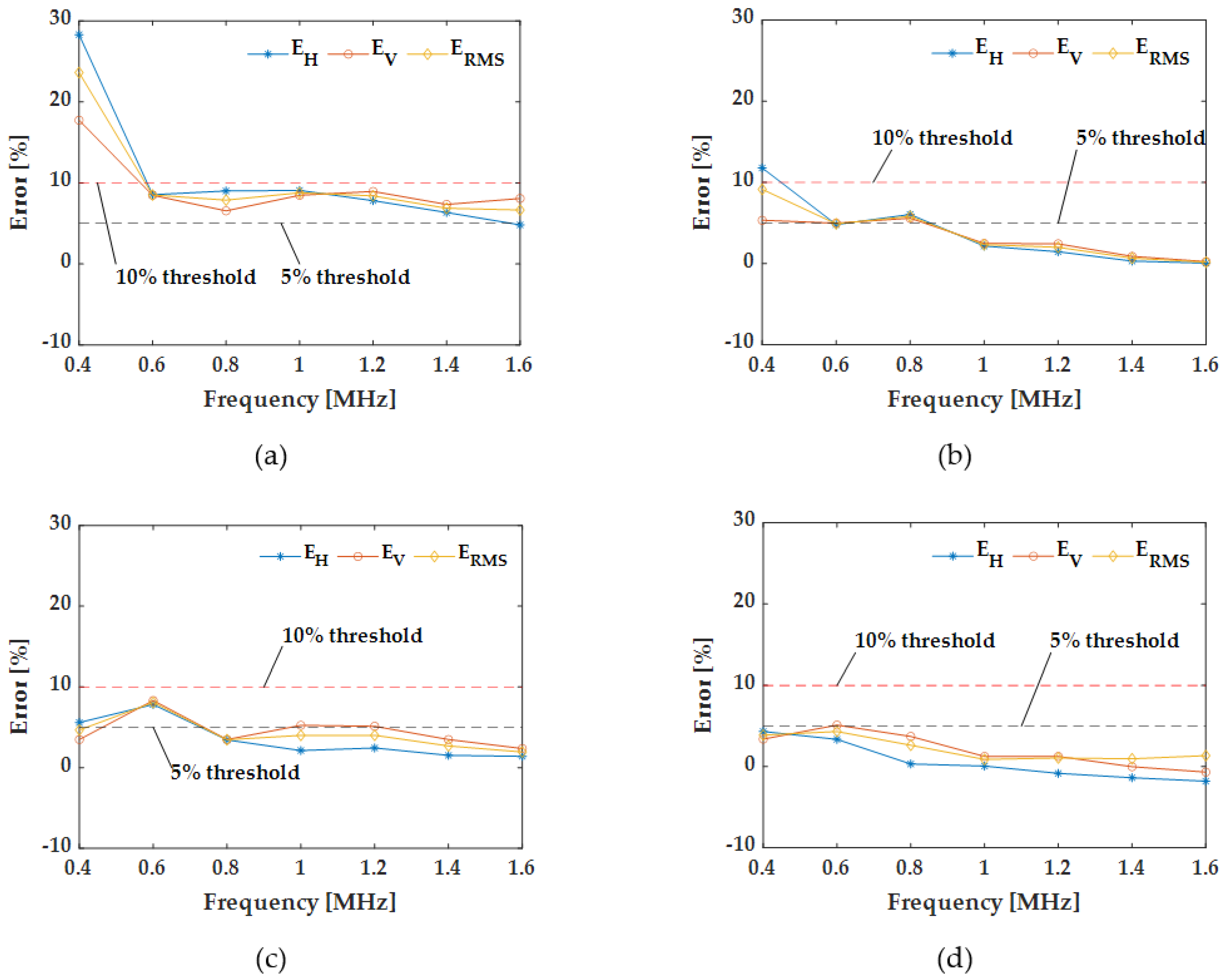
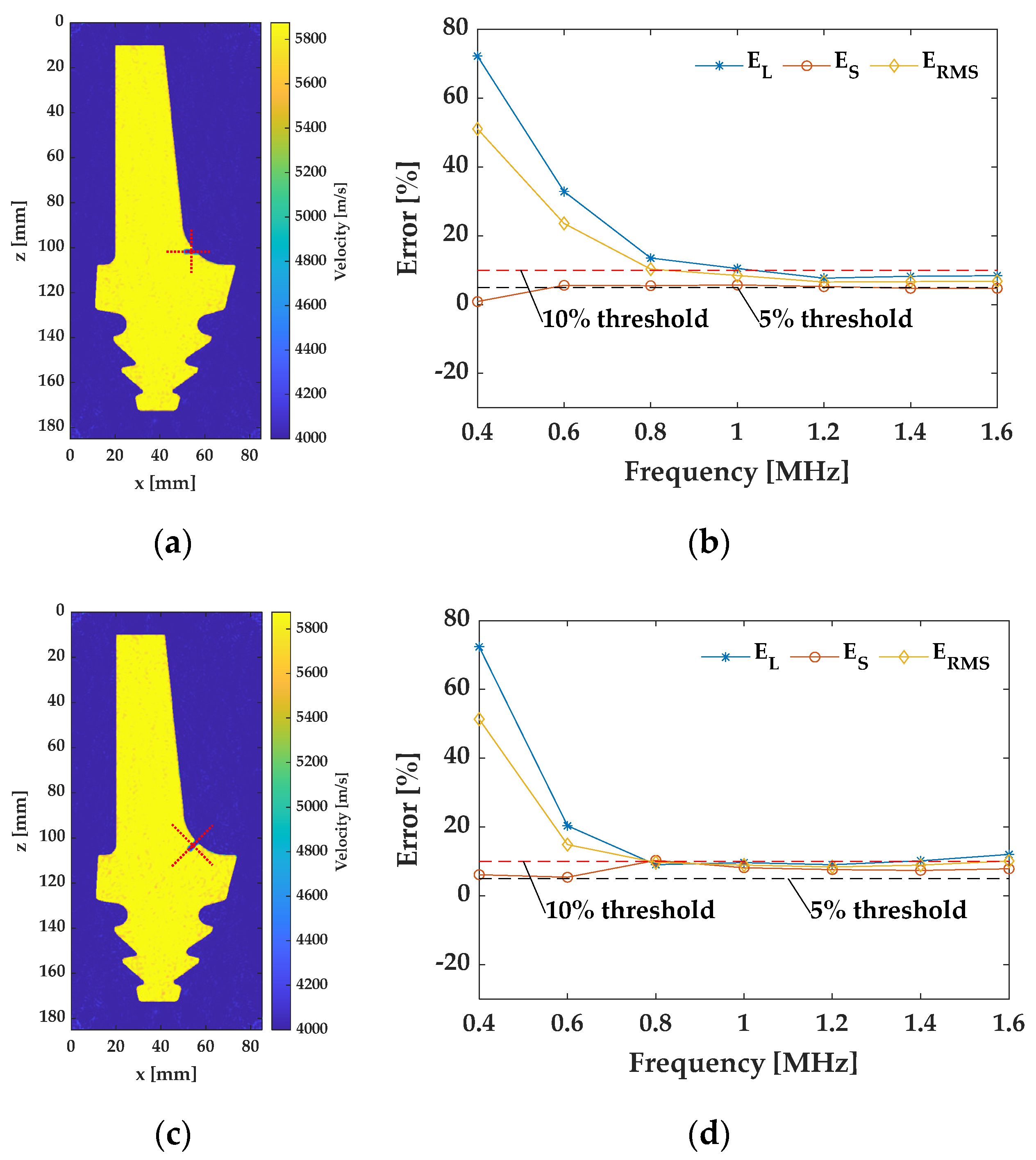
4.4. Uncertainty Analysis

Although a successive-frequency FWI shows a high accuracy in quantitative defect evaluation in a complex structure, an accurate or reliable initial model is very important for FWI. In previous studies, the exact wave speed was applied in the initial model for the inversion process. However, accurate material properties are not always available and might vary with the practical environments. Therefore, an uncertainty analysis should be conducted to assess the robustness of the proposed method. Here, two initial models with a −2% and +2% error for the velocity of the turbine blade were considered. Without a loss of generality, an internal defect with a diameter of 4 mm, slightly larger than the half wavelength, was introduced for FWI.

The tomograph results are shown in Figure 16a,c. In both cases, this defect could be accurately reconstructed. Compared with Figure 9 in Section 4.1, the reconstruction results showed more background noise. From the comparison of the vertical and horizontal profiles, as shown in Figure 16b,d, the RMS error of the FWHM was 5.42% for the −2% error in the initial model and 8.23% for the +2% error in the initial model. Compared with the relative error, which was smaller than 2% in Section 4.1, the inaccuracy of the initial model increased the relative error for the inversion. Vice versa, accurate parameters for the initial model could improve the final result. Nevertheless, the overall error was smaller than 10% and it was acceptable for the practical application in NDT even with a slight variation in the initial model.

5. Conclusions

In this paper, an ice-coupled ultrasonic tomography based on successive-frequency full waveform inversion technology was proposed to quantitively inspect the defects in complex-shaped parts. An ice-coupled ultrasound was able to treat the complex-shaped part as a regular structure and sharply reduced the mismatch of acoustic impedance compared with the immersion method. A series of numerical experiments were carried out to demonstrate the feasibility of the proposed method to quantitatively inspect the defects in a turbine blade. Firstly, the k-space pseudospectral method was applied to simulate ice-coupled ultrasonic testing for the turbine blade. A full matrix capture was then performed to record the ultrasonic signals with an evenly deployed transducer array. After data calibration, the recorded full wavefield was applied for a frequency-domain full waveform inversion based on the L-BFGS method. A single circular defect was applied to validate the proposed method and determine the iterative number and frequency. Compared with the monochromatic inversion, successive-frequency FWI could obtain more accurate results and the resolution approached a half wavelength. When the defects were larger than a half wavelength, the relative error was smaller than 2%. Extended studies on open notch cracks with different orientations and multiple adjacent defects proved that the proposed method was able to quantitatively detect various types of defects. Finally, inaccurate initial velocity models with a relative error of ±2% were also investigated. Despite the relative error increasing slightly, the proposed method was able to reconstruct the defects even with a certain inaccuracy. The results demonstrated that the ice-coupled ultrasonic FWI method has a high potential to quantitatively inspect complex-shaped structures with an excellent resolution.

It should be noted that a mode conversion in a practical ultrasonic test was not considered in this paper. In the future, an elastic wave equation should be considered in the forward model during the inversion process to obtain more accurate results and a practical experiment will be conducted.

References

1. Ravi-Kumar, B.V.R. A review on BLISK technology. Int. J. Innov. Res. Sci. Eng. Technol. 2013, 2, 1353–1358. [Google Scholar]
2. Pérez, M.; Carou, D.; Rubio, E.M.; Teti, R. Current advances in additive manufacturing. Procedia CIRP 2020, 88, 439–444. [Google Scholar] [CrossRef]
3. Brath, A.J.; Simonetti, F. Phased Array Imaging of Complex-Geometry Composite Components. IEEE Trans. Ultrason. Ferroelectr. Freq. Control. 2017, 64, 1573–1582. [Google Scholar] [CrossRef] [PubMed]
4. Fletcher, S.; Lowe, M.J.S.; Ratassepp, M.; Brett, C. Detection of Axial Cracks in Pipes Using Focused Guided Waves. J. Nondestruct. Eval. 2011, 31, 56–64. [Google Scholar] [CrossRef]
5. Moreau, L.; Drinkwater, B.W.; Wilcox, P.D. Ultrasonic imaging algorithms with limited transmission cycles for rapid nondestructive evaluation. IEEE Trans. Ultrason. Ferroelectr. Freq. Control 2009, 56, 1932–1944. [Google Scholar] [CrossRef] [PubMed]
6. Holmes, C.; Drinkwater, B.; Wilcox, P. The post-processing of ultrasonic array data using the total focusing method. Insight Non Destr. Test. Cond. Monit. 2004, 46, 677–680. [Google Scholar] [CrossRef]
7. Le Jeune, L.; Robert, S.; Villaverde, E.L.; Prada, C. Plane Wave Imaging for ultrasonic non-destructive testing: Generalization to multimodal imaging. Ultrasonics 2016, 64, 128–138. [Google Scholar] [CrossRef] [PubMed] [Green Version]
8. Ji, X.; Yuan, M.; Chen, Y. Cloud Ultrasound System with Flexible Ultrasonic Phased-Array Transducer for Critical Component Monitoring. In Proceedings of the International Symposium on Structural Health Monitoring and Nondestructive Testing 2018, Saarbruecken, Germany, 4–5 October 2018. [Google Scholar]
9. Jansen, D.; Hutchins, D. Immersion tomography using Rayleigh and Lamb waves. Ultrasonics 1992, 30, 245–254. [Google Scholar] [CrossRef]
10. Simonetti, F.; Satow, I.L.; Brath, A.J.; Wells, K.C.; Porter, J.; Hayes, B.; Davis, K. Cryo-Ultrasonic NDE: Ice–Cold Ultrasonic Waves for the Detection of Damage in Complex-Shaped Engineering Components. IEEE Trans. Ultrason. Ferroelectr. Freq. Control 2018, 65, 638–647. [Google Scholar] [CrossRef]
11. Simonetti, F.; Fox, M. Experimental methods for ultrasonic testing of complex-shaped parts encased in ice. NDT E Int. 2019, 103, 1–11. [Google Scholar] [CrossRef]
12. Tarantola, A. A strategy for nonlinear elastic inversion of seismic reflection data. Geophysics 1986, 51, 1893–1903. [Google Scholar] [CrossRef]
13. Pratt, R.G.; Worthington, M.H. Inverse theory applied to multi-source cross-hole tomography. Part 1: Acoustic wave-equation method. Geophys. Prospect. 1990, 38, 287–310. [Google Scholar] [CrossRef]
14. Pan, G.S.; Phinney, R.A.; Odom, R.I. Full-waveform inversion of plane-wave seismograms in stratified acoustic media: Theory and feasibility. Geophysics 1988, 53, 21–31. [Google Scholar] [CrossRef]
15. Pratt, R.G. Seismic waveform inversion in the frequency domain, Part 1: Theory and verification in a physical scale model. Geophysics 1999, 64, 888–901. [Google Scholar] [CrossRef] [Green Version]
16. Pérez-Liva, M.; Herraiz, J.L.; Udías, J.M.; Miller, E.; Cox, B.T.; Treeby, B.E. Time domain reconstruction of sound speed and attenuation in ultrasound computed tomography using full wave inversiona. J. Acoust. Soc. Am. 2017, 141, 1595–1604. [Google Scholar] [CrossRef] [Green Version]
17. Bernard, S.; Monteiller, V.; Komatitsch, D.; Lasaygues, P.L. Ultrasonic computed tomography based on full-waveform inversion for bone quantitative imaging. Phys. Med. Biol. 2017, 62, 7011–7035. [Google Scholar] [CrossRef]
18. Nguyen, T.D.; Tran, K.T.; Gucunski, N. Detection of Bridge-Deck Delamination Using Full Ultrasonic Waveform Tomography. J. Infrastruct. Syst. 2017, 23, 04016027. [Google Scholar] [CrossRef]
19. Nguyen, L.T.; Modrak, R.T. Ultrasonic wavefield inversion and migration in complex heterogeneous structures: 2D numerical imaging and nondestructive testing experiments. Ultrasonics 2018, 82, 357–370. [Google Scholar] [CrossRef]
20. Rao, J.; Ratassepp, M.; Fan, Z. Limited-view ultrasonic guided wave tomography using an adaptive regularization method. J. Appl. Phys. 2016, 120, 194902. [Google Scholar] [CrossRef]
21. Rao, J.; Ratassepp, M.; Fan, Z. Guided Wave Tomography Based on Full Waveform Inversion. IEEE Trans. Ultrason. Ferroelectr. Freq. Control 2016, 63, 737–745. [Google Scholar] [CrossRef] [PubMed]
22. Brossier, R.; Operto, S.; Virieux, J. Seismic imaging of complex onshore structures by 2D elastic frequency-domain full-waveform inversion. Geophysics 2009, 74, WCC105–WCC118. [Google Scholar] [CrossRef]
23. Jo, C.H.; Shin, C.; Suh, J. An optimal 9-point, finite-difference, frequency-space, 2-D Scalar wave extrapolator. Geophysics 1996, 61, 529–537. [Google Scholar] [CrossRef] [Green Version]
24. Chen, Z.; Cheng, D.; Feng, W.; Wu, T. An optimal 9-point finite difference scheme for the Helmholtz equation with PML. Int. J. Numer. Anal. Model. 2013, 10, 389–410. [Google Scholar] [CrossRef] [Green Version]
25. Pratt, R.G. Frequency-domain elastic wave modeling by finite differences: A tool for crosshole seismic imaging. Geophysics 1990, 55, 626–632. [Google Scholar] [CrossRef]
26. Belanger, P.; Cawley, P.; Simonetti, F. Guided wave diffraction tomography within the born approximation. IEEE Trans. Ultrason. Ferroelectr. Freq. Control 2010, 57, 1405–1418. [Google Scholar] [CrossRef]
27. Norton, S.J. Iterative inverse scattering algorithms: Methods of computing Fréchet derivatives. J. Acoust. Soc. Am. 1999, 106, 2653–2660. [Google Scholar] [CrossRef]
28. Guitton, A.; Symes, W.W. Robust inversion of seismic data using the Huber norm. Geophysics 2003, 68, 1310–1319. [Google Scholar] [CrossRef]
29. Huthwaite, P.; Simonetti, F. High-resolution guided wave tomography. Wave Motion 2013, 50, 979–993. [Google Scholar] [CrossRef]
30. Treeby, B.E.; Cox, B.T. K-Wave: MATLAB toolbox for the simulation and reconstruction of photoacoustic wave fields. J. Biomed. Opt. 2010, 15, 021314. [Google Scholar] [CrossRef]
31. Lowe, M.J.S.; Alleyne, D.N.; Cawley, P. The Mode Conversion of a Guided Wave by a Part-Circumferential Notch in a Pipe. J. Appl. Mech. 1998, 65, 649–656. [Google Scholar] [CrossRef]
32. Leonard, K.R.; Malyarenko, E.V.; Hinders, M.K. Ultrasonic Lamb wave tomography. Inverse Probl. 2002, 18, 1795–1808. [Google Scholar] [CrossRef]
Figure 1. Workflow of the ultrasonic full waveform inversion algorithm.
Applsci 11 04433 g001
Figure 2. (a) Photo of a turbine blade and (b) typical cross section.
Applsci 11 04433 g002
Figure 3. Configuration of the ultrasonic transducer array.
Applsci 11 04433 g003
Figure 4. Excitation signal ( f c = 1   MHz and t 0 = 1.5 / f c ). (a) Waveform in the time domain and (b) the corresponding normalized amplitude spectrum.
Applsci 11 04433 g004
Figure 5. Ultrasonic wave propagation excited with the 1 st transducer at different time slots: (a) t = 6   μ s ; (b) = 8   μ s ; (c) = 21   μ s ; (d) = 26   μ s .
Applsci 11 04433 g005
Figure 6. The recorded signal of the 19 th transducer excited with the 1 st transducer. (a) The A-scan waveform and (b) the corresponding amplitude spectrum.
Applsci 11 04433 g006
Figure 7. The evolution of the objective function with the number of iterations.
Applsci 11 04433 g007
Figure 8. (a) True model with a 3 mm circular hole and tomographs with different iterations: (b) k = 5; (c) k = 10; (d) k = 20; (e) k = 40.
Applsci 11 04433 g008
Figure 9. Tomographs of the 3 mm circular hole based on successive-frequency inversions at: (a) 0.4 MHz; (b) 0.6 MHz; (c) 0.8 MHz; (d) 1 MHz; (e) 1.2 MHz; (f) 1.4 MHz; (g) 1.6 MHz.
Applsci 11 04433 g009
Figure 10. Cross sections of the reconstruction of the 3 mm diameter circular hole along the (a) horizontal and (b) vertical direction.
Applsci 11 04433 g010
Figure 11. The variation of relative errors of the FWHM as a function of successive-frequency inversions for circular holes: (a) 3 mm; (b) 4 mm; (c) 5 mm; (d) 6 mm.
Applsci 11 04433 g011
Figure 12. Inversion results for open notch cracks. Tomograph and error variation for (a,b) the horizontal notch, (c,d) the inclined notch at 45° and (e,f) the vertical notch.
Applsci 11 04433 g012aApplsci 11 04433 g012b
Figure 13. (a) True model and (b) FWI tomograph of three defects.
Applsci 11 04433 g013
Figure 14. Cross sections (a) through #1 and #2 defects and (b) through #3 defect along the horizontal direction. Cross sections (c) through #1 and #3 defects and (d) through #2 defect along the vertical direction.
Applsci 11 04433 g014
Figure 15. (a) FWI tomograph of three circular holes and a notch defect. Cross section (b) through the incline notch along the width direction, (c) through #1 and #2 defects along the horizontal direction and (d) through #3 defect along the horizontal direction. The positions are depicted in (a) with red dashed lines.
Applsci 11 04433 g015
Figure 16. Inversion results with an inaccurate initial model. (a) Tomograph and (b) horizontal profile for an initial model with a −2% error. (c) Tomograph and (d) horizontal profile for an initial model with a +2% error.
Applsci 11 04433 g016