Coherent Image Source Modeling of Sound Fields in Long Spaces with a Sound-Absorbing Ceiling ^†

Abstract

Sound-absorbing boundaries can attenuate noise propagation in practical long spaces, but fast and accurate sound field modeling in this situation is still difficult. This paper presents a coherent image source model for simple yet accurate prediction of the sound field in long enclosures with a sound absorbing ceiling. In the proposed model, the reflections on the absorbent boundary are separated from those on reflective ones during evaluating reflection coefficients. The model is compared with the classic wave theory, an existing coherent image source model and a scale-model experiment. The results show that the proposed model provides remarkable accuracy advantage over the existing models yet is fast for sound prediction in long spaces.

1. Introduction

Sound prediction is very important for design of practical long spaces such as traffic tunnels and subway stations to evaluate acoustical qualities such as speech intelligibility of public address systems [1]. For noise control in such long spaces, it is often the case to apply acoustical liners to the space ceiling for larger noise attenuation. Regarding sound prediction in such spaces, classic room acoustics formulas are unsatisfactory [2,3] because the sound field is not diffused due to the extreme dimensions. The commonly used incoherent geometrical acoustics models [4,5,6,7,8] cannot account for the interference between multiple sound reflections on impedance boundaries, which were experimentally observed to be distinct and can notably affect the sound prediction accuracy in this situation [3,9,10], especially at lower frequencies and in early parts of the impulse response [10].

For the coherent geometrical acoustics models, Li et al. developed a numerical model for coherent sound prediction inside long spaces [3,11] and afterwards applied this prediction model into full-scale tunnels [9] and a long space with impedance discontinuities [12]. It was shown that their coherent prediction model provides much better prediction accuracy than the usual incoherent ones for long spaces with reflective boundaries. However, for applications with sound-absorbing boundaries, the applicability of their model may be limited. The numerical model of Li et al. [3] originated from a coherent image source method by Lemire and Nicolas [13], in which it is implicitly assumed that the wave front shapes remain spherical during each successive reflection of the initial spherical wave radiation [13]. This assumption may hardly hold for reflections on sound-absorbing boundaries.

Recently, Min et al. [14] proposed a coherent image source method for fast yet accurate sound prediction in flat spaces with absorbent boundaries. They proposed different refection coefficients to evaluate the reflections on the absorbent and reflective boundaries, which avoids the prediction difficulties with absorbent boundaries in the method of Lemire and Nicolas. Unfortunately, their model is currently limited to spaces with two parallel infinite boundaries in theory.

Upon reviewing the studies above, there is still the problem of sound prediction in long spaces with sound-absorbing boundaries for practical noise control. In this paper, a coherent image source model is extended and examined theoretically and experimentally for fast yet accurate sound prediction in long spaces with sound-absorbing boundaries.

2. Theoretical Method

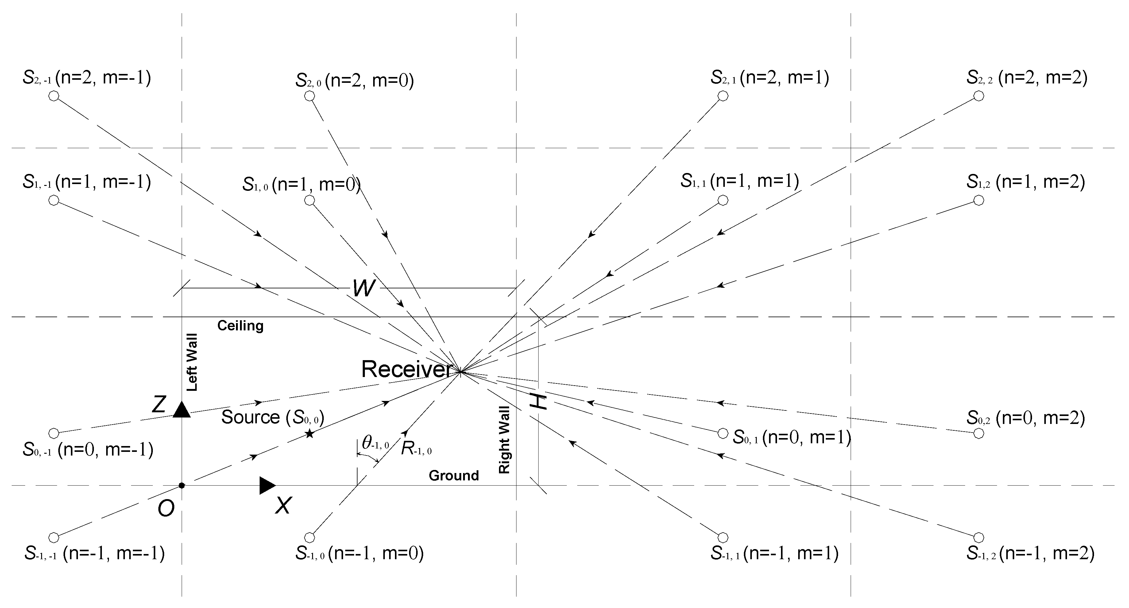
Figure 1 shows the cross-sectional geometry of a long rectangular space with a height of H and width W. For simplicity, four boundaries in this space, the ceiling, ground, and right and left walls, are assumed to be locally reactive with a uniform normalized specific admittance of β_c, β_g, β_r, and β_l, respectively. The ceiling is defined to be sound absorptive with a relatively high sound absorption coefficient, while other boundaries are sound reflective with a relatively low absorption coefficient. The space extends infinitely along the y-direction as a typical case and a point source is located at (x_S, 0, z_S) and a receiver is located at (x_r, y_r, z_r) inside.

To model the sound field, we first assume that kW >> 1 and kH >> 1 (with k for the wavenumber) so that the boundaries may be considered infinity for each sound reflection on them [13]. The total sound pressure field at receiver can be approximated as a summation of successive sound reflections on four boundaries:

$$P_{tot}\approx {\displaystyle \sum _{n=-\infty }^{+\infty }{\displaystyle \sum _{m=-\infty }^{+\infty }{P}_{n,m}}}$$

(1)

where n, m = 0, ±1, ±2, …, and P_n,m represents the sound field contribution from the (n, m)-th order image source, in which a positive n (or m) is for an image source located above the ceiling (or rightwards from the right wall) while a negative n (or m) is for that located below the floor (or leftwards from the left wall), as shown in Figure 1. Particularly, P_0,0 denotes the direct sound from the real source S_0,0. Based on the assumption of kW >> 1 and kH >> 1, P_n,m can be approximated from the plane wave expansion of a spherical wave as follows [14,15]:

$$P_{n,m}\approx \frac{jk}{8{\pi }^2}{\displaystyle {\int }_0^{2\pi }{\displaystyle {\int }_0^{\frac{\pi }{2}-j\infty }{e}^{jk\cdot R_{n,m}}}}{[V_g(\theta )]}^{n_g}{[V_c(\theta )]}^{n_c}{[V_l(\alpha )]}^{m_l}{[V_r(\alpha )]}^{m_r}\sin \theta d\theta d\varphi$$

(2)

where n_g, n_c, m_l, and m_r are used to count reflection times on the ground, ceiling, and left and right walls in the path from S_n,m to the receiver, respectively. They can be determined from the order (n, m) by

$$\begin{gathered} n_{g,c}=\frac{\left|n\right|}{2}\mp \frac{1}{2}\mathrm{sign}(n)\mathrm{rem}(|n|,2) \\ {m}_{l,r}=\frac{\left|m\right|}{2}\mp \frac{1}{2}\mathrm{sign}(m)\mathrm{rem}(|m|,2) \end{gathered}$$

(3)

In Equation (2), R_n,m= (R_n,_msinθ_n,_mcosj_n,m, R_n,msinθ_n,_msinj_n,m, R_n,_mcosθ_n,m) represents the distance vector from S_n,m to the receiver, with explicit azimuth angles θ_n,m and j_n,m. V_g(θ) and V_c(j) are the plane wave reflection coefficients on the “infinite” ground and ceiling with the incidence angle θ, respectively, while V_l(α) and V_r(α) are those on the left and right walls with the incidence angle α = π/2−θ, respectively. These plane wave reflection coefficients can be correspondingly evaluated by [16]

$$V_{g,c,r,l}(\zeta )=\frac{\cos \zeta -{\beta }_{g,c,r,l}}{\cos \zeta +{\beta }_{g,c,r,l}}$$

(4)

Through an identical mathematical transformation similar to that from Equations (8)–(12) in Ref. [14], the evaluation of P_n,m in Equation (2) can be simplified as

$$P_{n,m}\approx \frac{jk}{8\pi }{\displaystyle {\int }_{-\frac{\pi }{2}+j\infty }^{\frac{\pi }{2}-j\infty }V(\theta )\sin \theta \cdot H_0^1(kr\sin \theta ) e^{jk{R}_{n,m}\cos \theta \cos {\theta }_{n,m}}d\theta }$$

(5)

where V(θ) represents the term ${[V_g(\theta )]}^{n_g}{[V_c(\theta )]}^{n_c}{[V_l(\alpha )]}^{m_l}{[V_r(\alpha )]}^{m_r}$, r = R_n,msinθ_n,_m, and $H_0^1(.)$ is the first Hankel function with zero-th order. In Equation (5), the ray field from single reflection on the reflective boundaries, P_−1,0 for example, can be further evaluated as [13,17]

$$P_{-1,0}=Q_{ref}(S_{-1,0},R|\mathrm{GB})\cdot \frac{e^{jk{R}_{-1,0}}}{4\pi R_{-1,0}}$$

(6)

where $Q_{ref}(S_{-1,0},R|\mathrm{GB})$ represents the single reflection coefficient on the reflective ground boundary (GB) and is evaluated as [13,17]

$$Q_{ref}(S_{-1,0},R|\mathrm{GB})=V_g({\theta }_{-1,0})+[1-V_g({\theta }_{-1,0})]F(w_n),$$

(7)

in which

$$F(w_n)=1+j\sqrt{\pi }\cdot w_n\cdot g(w_n),$$

(8)

$$w_n=\sqrt{k{R}_{-1,0}}\cdot \frac{1+j}{2}\cdot (\cos {\theta }_{-1,0}+{\beta }_g), \mathrm{and}$$

(9)

$$g(w_n)=e^{-w_n{}^2}\mathrm{erfc}\left(j{w}_n\right).$$

(10)

Further analytical approximation of g (w_n) is available in Ref. [18].

It was shown that the wave front shape before and after each reflection on the reflective boundaries can almost remain the same [14,19]. This suggests that single reflection coefficients Q_ref shall be weakly dependent on θ and be almost uniform for different spatial parts of incident wave fronts of any shapes [14]. Accordingly, during the ray propagation from S_n,m to receiver in Figure 1, the evaluation of each reflection upon one reflective boundary (or each “transmission” through it or its images) can be approximated by once-weighting the ray field with the corresponding single reflection coefficient Q_ref on this boundary [14]. Thus, after the ray field being weighted for n_g, m_l, and m_r times due to “transmission” through the reflective ground, left wall (LW) and right wall (RW), and their images, the evaluation of P_n,m can be simplified by

$$\begin{gathered} P_{n,m}\approx {[Q_{ref}(S_{n,m},R|\mathrm{GB})]}^{n_g}\cdot {[Q_{ref}(S_{n,m},R|\mathrm{LW})]}^{m_l}\cdot {[Q_{ref}(S_{n,m},R|\mathrm{RW})]}^{m_r} \\ \cdot \frac{jk}{8\pi }{\displaystyle {\int }_{-\frac{\pi }{2}+j\infty }^{\frac{\pi }{2}-j\infty }{[V_c(\theta )]}^{n_c}\sin \theta \cdot H_0^1(kr\sin \theta ) e^{jk{R}_{n,m}\cos \theta \cos {\theta }_{n,m}}d\theta }, \end{gathered}$$

(11)

where the integral involves only the reflection coefficient on the absorptive ceiling boundary (CB) and can be further evaluated through the second order approximation provided by Brekhovskikh [15] to yield

$$\begin{gathered} P_{n,m}\approx {[Q_{ref}(S_{n,m},R|\mathrm{GB})]}^{n_g}\cdot {[Q_{ref}(S_{n,m},R|\mathrm{LW})]}^{m_l}\cdot {[Q_{ref}(S_{n,m},R|\mathrm{RW})]}^{m_r} \\ \cdot \left\{V_t({\theta }_{n,m}|\mathrm{CB},n_c)-\frac{j\left[{V^{\prime }}_t({\theta }_{n,m}|\mathrm{CB},n_c)\cot {\theta }_{n,m}+{V^{″}}_t({\theta }_{n,m}|\mathrm{CB},n_c)\right]}{2k{R}_{n,m}}\right\}\cdot \frac{e^{jk{R}_{n,m}}}{4\pi R_{n,m}}, \end{gathered}$$

(12)

where V_t(θ_n,m|CB, n_c) = [V_c(θ_n,m)]^nc, and ${V^{\prime }}_t({\theta }_{n,m}|\mathrm{CB},n_c)$ and ${V^{″}}_t({\theta }_{n,m}|\mathrm{CB},n_c)$ are the first and second derivatives of V_t(θ_n,m|CB, n_c) at θ_n,m, respectively. This equation may be rewritten as an image source model form as

$$P_{n,m}=Q_{n,m}\frac{e^{jk{R}_{n,m}}}{4\pi R_{n,m}},$$

(13)

where Q_n,m represents a combined reflection coefficient corresponding to the ray with reflection order (n,m) as

$$\begin{gathered} Q_{n,m}={[Q_{ref}(S_{n,m},R|\mathrm{GB})]}^{n_g}\cdot {[Q_{ref}(S_{n,m},R|\mathrm{LW})]}^{m_l} \\ \cdot {[Q_{ref}(S_{n,m},R|\mathrm{RW})]}^{m_r}\cdot Q_{abs}(S_{n,m},R|\mathrm{CB},n_c) \end{gathered}$$

(14)

in which Q_abs (S_n,m, R| CB, n_c) represents one reflection coefficient accounting for overall effect from successive reflections on the absorptive ceiling boundary as

$$Q_{abs}(S_{n,m},R|\mathrm{CB},n_c)\approx V_t({\theta }_{n,m}|\mathrm{CB},n_c)-\frac{j\left[{V^{\prime }}_t({\theta }_{n,m}|\mathrm{CB},n_c)\cot {\theta }_{n,m}+{V^{″}}_t({\theta }_{n,m}|\mathrm{CB},n_c)\right]}{2k{R}_{n,m}}$$

(15)

One can easily expand Q_abs (S_n,m, R| CB, n_c) for analytical evaluation, and this is not presented here for succinctness. Equations (1), (13), and (14) provide a coherent image source model for long rectangular spaces with a sound-absorbent ceiling.

3. Results and Discussion

Numerical simulations are firstly carried out to validate the proposed coherent image source model. As the classic wave theory is analytically exact in the spaces studied in this paper [16], it is used as a reference method to provide benchmark results in validations. The coherent image source method by Lemire and Nicolas [13] that was widely used in previous studies [3,9,12] is also investigated for comparisons. Numerical implementation of the methods above stays similar to that in Refs. [13,14], except the geometry of four boundaries in Figure 1.

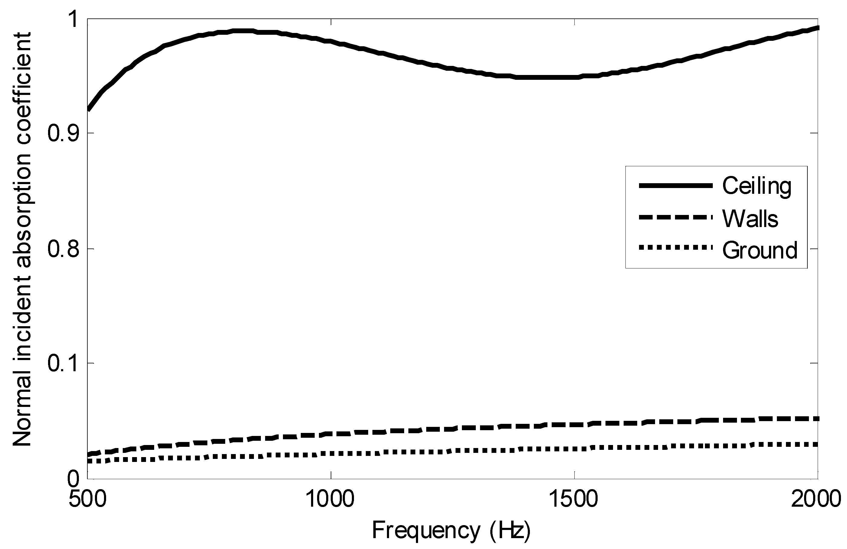
In simulations, a long rectangular space with W × H = 20 m × 5 m is considered to simulate one city road tunnel with four lanes. For simplicity, four tunnel boundaries are all assumed to be rigidly backed layers of homogeneous porous material. Attenborough’s “three-parameter” approximation [14,20] is applied to evaluate surface admittances for these boundaries, in which the boundary media parameters of flow resistivity (σ), porosity (Ω), tortuosity (T), pore shape factor (S_p), and thickness (d) are used for evaluation. The tunnel ceiling is defined as highly sound absorptive, with σ = 10 cgs (where 1 cgs = 1 kPa s m⁻²), Ω = 1, T = 1, S_p = 0.25, and d = 0.1 m, such as a wool layer. The ground has σ = 10 k cgs, Ω = 0.2, T = 1.4, S_p = 0.5, and d = 0.05 m to represent a compact asphalt pavement layer. The right and left walls have σ = 0.5 k cgs, Ω = 0.1, T = 1, S_p = 0.3, and d = 0.01 m to represent cement plaster over concrete walls. Figure 2 shows the corresponding normal incident absorption coefficients of these four boundaries in simulations.

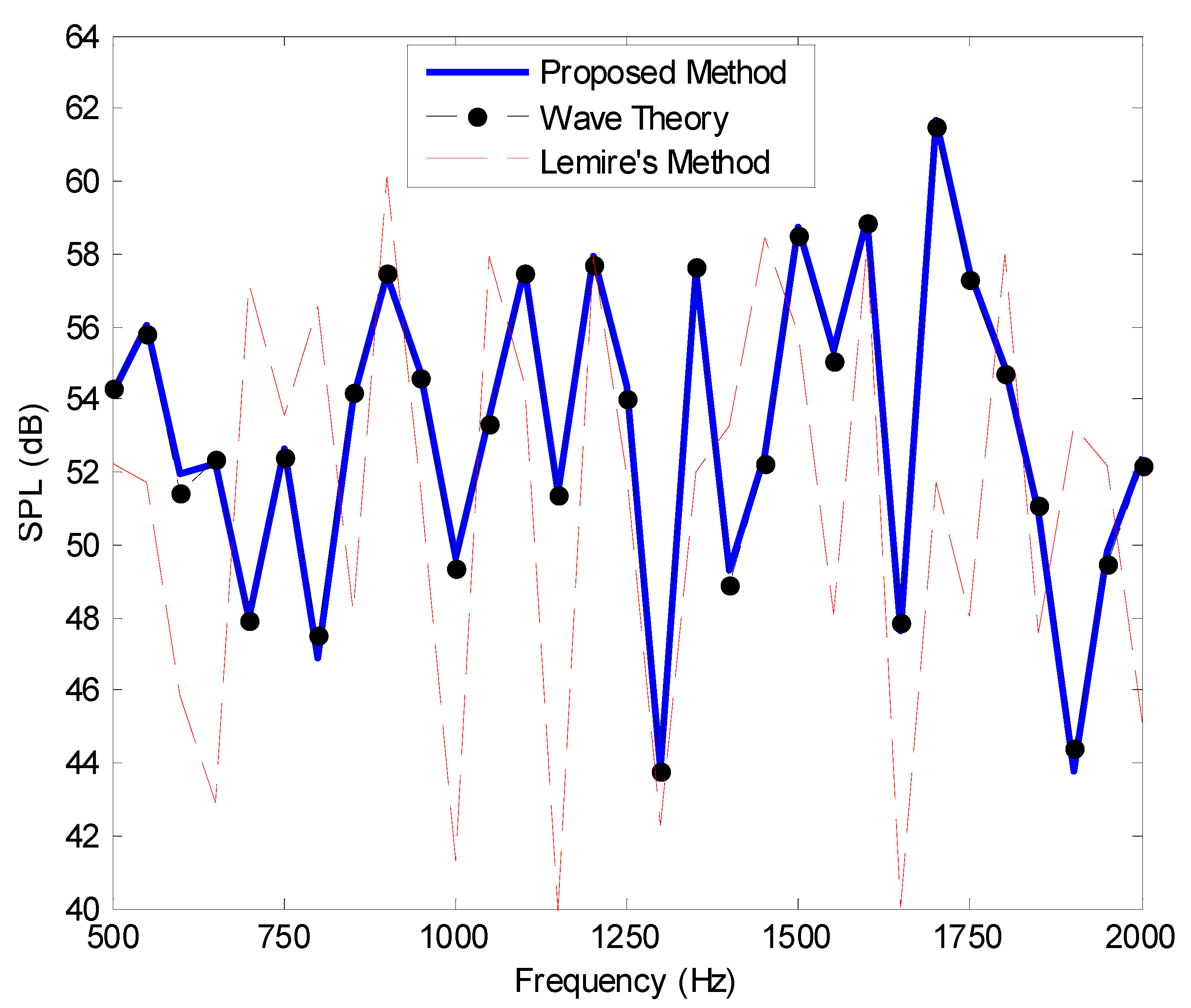
Two sets of numerical simulations are conducted. In the first set, predictions of sound pressure level (SPL) spectrum at the receiver (6 m, 50 m, 1 m) from a point source at (6 m, 0 m, 1 m) are investigated. Predictions from the proposed method, the wave theory, and the method of Lemire and Nicolas are compared in Figure 3. It is shown that the results from the proposed method agree excellently with those of the wave theory over frequencies from 500 to 2000 Hz, with only small deviations (<1 dB) at few lower frequencies. This suggests the successful extension of the coherent image source method by Min et al. [14] for spaces enclosed by four perpendicular finite boundaries in this paper. It can also be observed from Figure 3 that the predictions with the method of Lemire and Nicolas differ significantly from the benchmark results over frequencies in this situation. This indicates that the existing coherent models [3,9,12] based on the method of Lemire and Nicolas can hardly be accurate in long spaces with absorbent boundaries because the assumption of spherical wave front shapes for each successive reflection is unsatisfied in this situation. All simulations are executed in Matlab 2010b on the same personal computer with a 2.4 GHz Intel Core i5-560M processor and 8 Gbytes of random access memory. Computational time records show that, for results at all the 31 frequencies in Figure 3, evaluation of the proposed model and the method of Lemire and Nicolas takes 50.3 s and 49.7 s, respectively, while the corresponding execution time with the wave theory takes over 2 h. This indicates the remarkable advantage of the proposed model both at accuracy and efficiency for sound predictions in long spaces with absorbent boundaries.

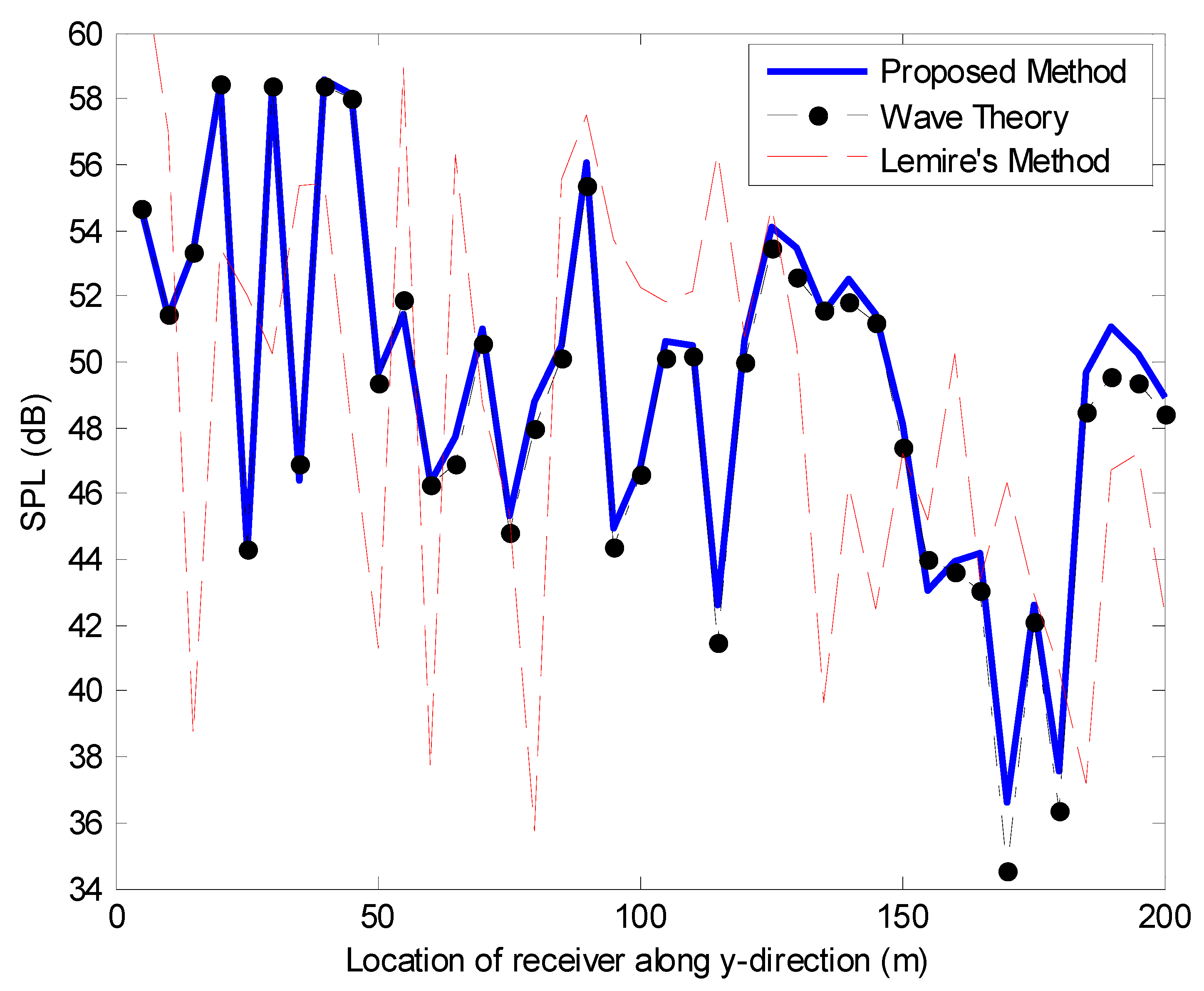
In the second simulation set, predictions of the SPL distribution inside the long rectangular space are investigated. Figure 4 presents SPL predictions at frequency of 1000 Hz versus the receiver location along the tunnel extension direction. The source is located at (6 m, 0 m, 1 m) and the receiver is located at (6 m, y_r, 1 m) with y_r moving from 5 m to 200 m along the space length-extending direction. From Figure 2, the absorption coefficients of the ceiling, ground, and walls at a frequency of 1000 Hz are 0.98, 0.02, and 0.04, respectively. Figure 4 shows remarkably good agreement between the proposed model and the wave theory, even at receiver locations far away from the source compared to the space height and width. However, large prediction differences can be found between the method of Lemire and Nicolas and the reference method in this situation. In Figure 4, prediction error from the proposed method increases at a longer source/receiver distance. The reason may be that, when the receiver moves farther away from the source compared to the space cross section dimensions, high-order reflection rays provide relatively higher contributions in the receiver total sound field. In the proposed model, reflection ray field is evaluated through Equations (13) and (14) by approximating each reflection at reflective boundaries as one single reflection. This may accumulate larger errors for higher-order reflection rays.

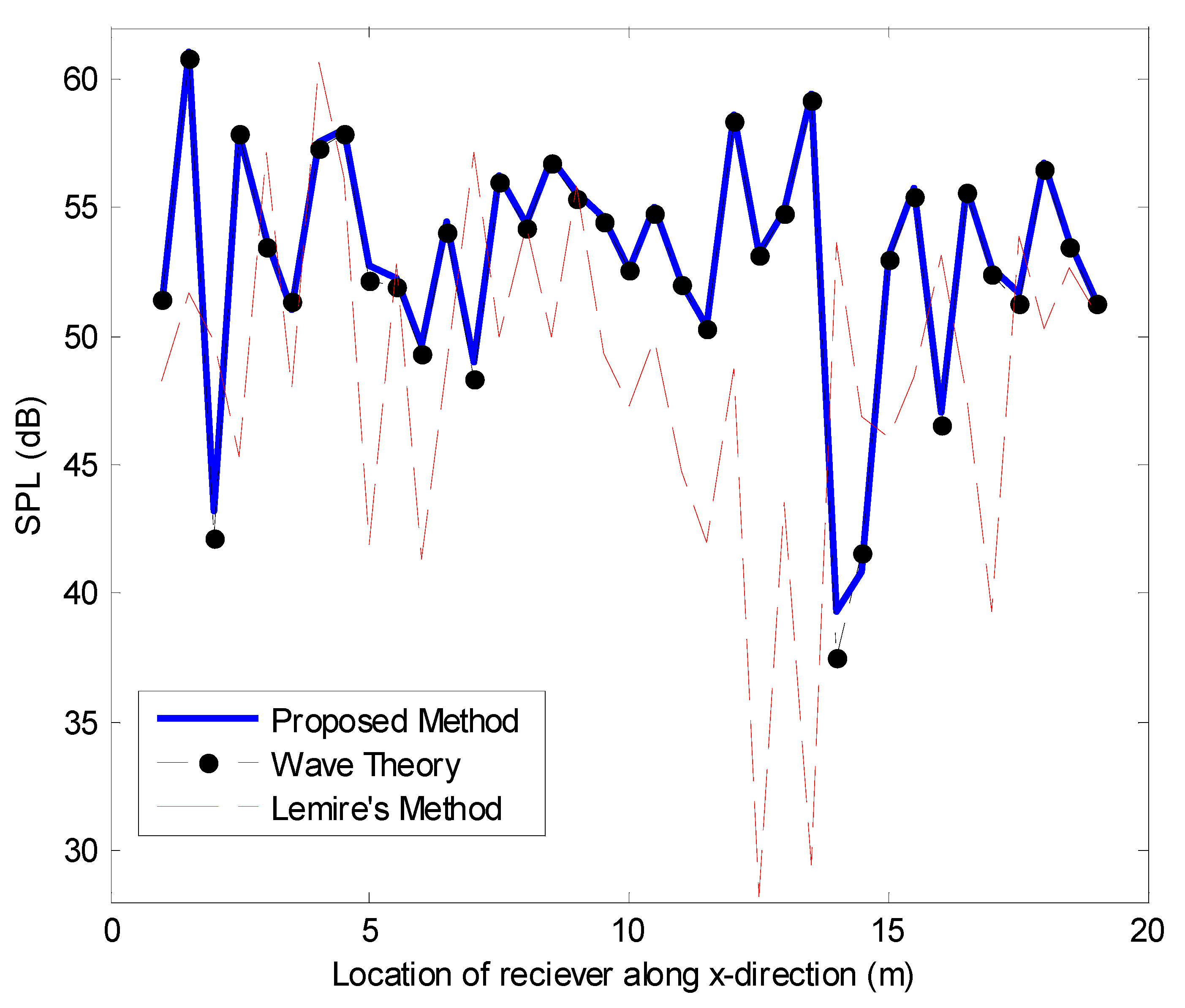
Figure 5 presents the SPL predictions at frequency of 1000 Hz versus the receiver location along the tunnel width direction. The source is located at (6 m, 0 m, 1 m) and the receiver is located at (x_r, 50 m, 1 m) with x_r moving from 1 m to 19 m. The results show excellent prediction agreement between the proposed model and the wave theory, even at receiver locations close to boundary interaction corners compared to the wavelength. 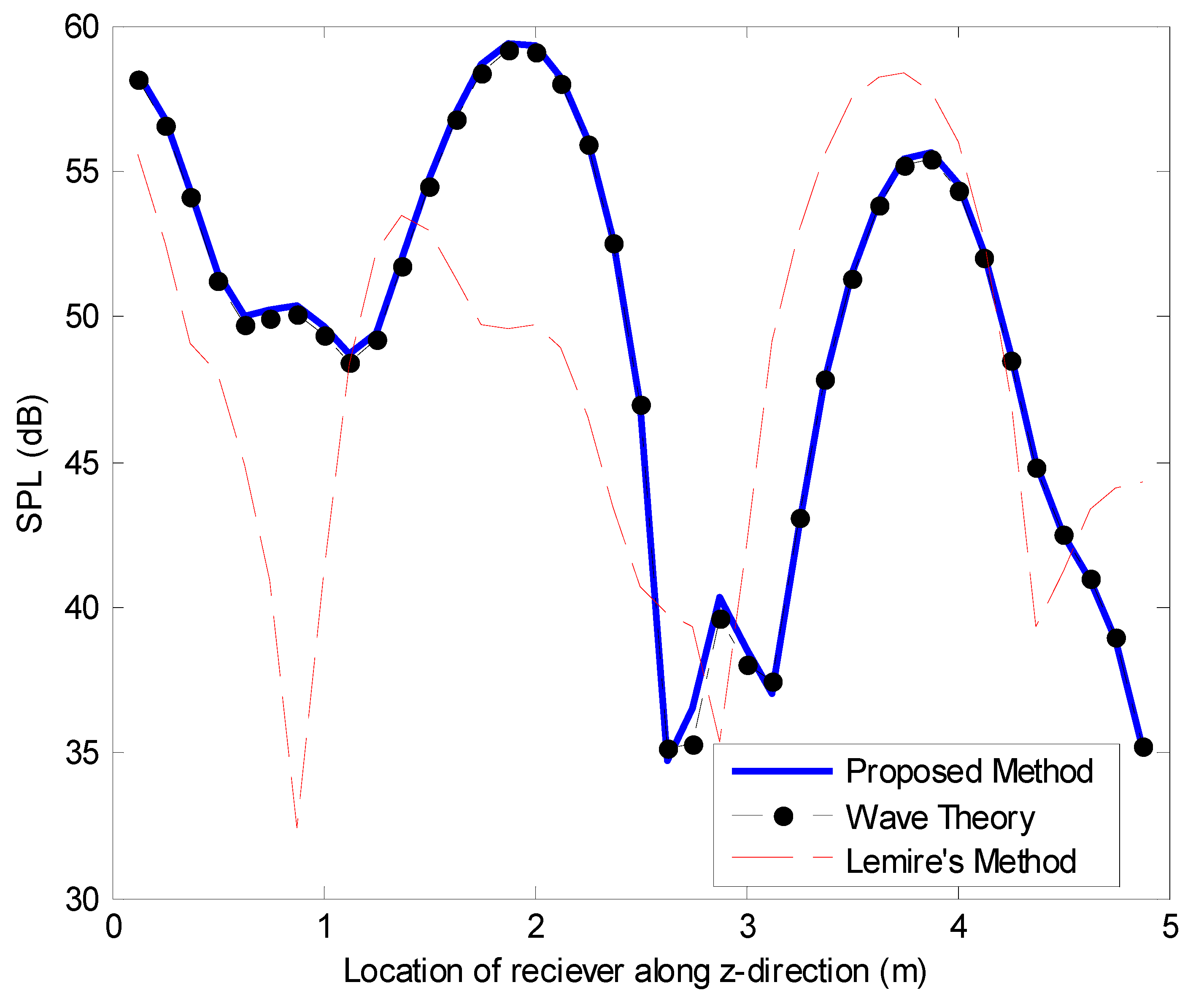In Figure 5, large discrepancies remain between the method of Lemire and Nicolas, and the reference method. Predictions are also compared on the SPL at 1000 Hz versus the receiver location along the tunnel height direction, with the source at (6 m, 0 m, 1 m) and the receiver at (6 m, 50 m, z_r) with z_r moving from 0.125 m to 4.875 m. The corresponding results are presented in Figure 6. It is shown that results from the proposed model almost overlap those from the wave theory, not only at receiver locations close to the reflective ground but also at those in the vicinity of the absorbent ceiling compared to the wavelength. Predictions with the method of Lemire and Nicolas still bias much from the benchmark results in this situation. The computational time in this simulation set is also recorded for comparison. In Matlab 2010b on the same computer as mentioned above, an evaluation of the proposed model and the method of Lemire and Nicolas takes about 1.8 s and 1.7 s for results at each receiver location in Figure 4 to Figure 6, respectively, while the corresponding calculation with the wave theory takes over 80 s. These show that the proposed coherent image source model can accurately predict the sound fields in long rectangular spaces with an absorbent ceiling, while its computational load stays at a same level with the existing models [3,9,12,13].

A scale-model experiment was carried out to further verify the predictions. One model long rectangular space was built with inner dimensions of 0.7 m width, 0.45 m height, and 10 m length for the measurements, which was scaled with 1:10 to represent a tunnel with W × H = 7 m × 4.5 m in full scale (all of the following dimensions referred to are scaled ones unless otherwise stated). Panels of 20 mm thick high-density fiberboard were used to build the model long space, and the model’s inner surfaces were well finished to represent sound reflective ground and wall boundaries. A layer of 50 mm thick fiberglass was used as a liner on the top panel to represent an absorbent ceiling. To minimize the sound reflection on the two ends of the model’s long space for infinite extension, liners of 200 mm thick fiberglass were applied onto those two end panels. The specific normalized admittances of the model boundaries were preliminarily measured through an impedance tube kit typed B&K 4206.

A speaker driver with a tube of internal diameter of 2 cm and length of 1 m was applied to represent a point source [3]. One microphone typed B&K 4190 was used as the receiver. Sound signals were generated and collected through one B&K Pulse system 3560D. In measurements, high enough levels of white noise were generated into the model long space to ensure the steady SPL at most locations inside remained at least 15 dB higher than the background noise. 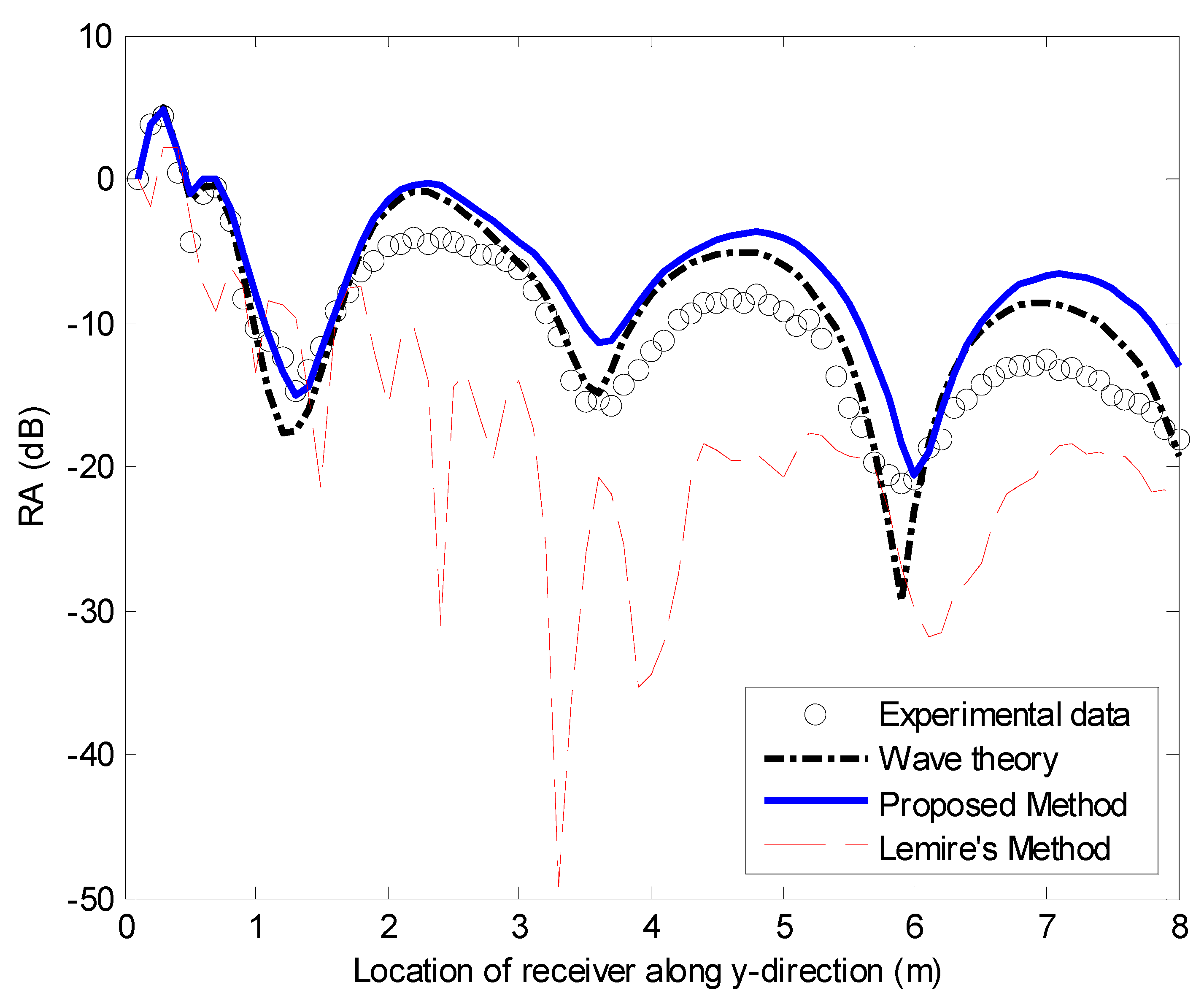In accordance with coordinates defined in Figure 1, in the experiment, the point source (the speaker tube mouth) was located at (0.35 m, 0 m, 0.2 m) and the receiver was located at (0.35 m, y_r, 0.1 m) with y_r moving from 0.1 m to 8 m to investigate the SPL distribution along the space extension direction. Relative attenuation (RA) was used to present the measured and predicted results in the experiment, which is defined as subtracting the SPL at (0.35 m, 0.1 m, 0.2 m) from that at receiver. The predictions from the wave theory that are used as benchmarks in simulations were firstly compared with the experimental data. Figure 7 presents the comparison results on the RA distribution along the y-direction. The frequency of 1000 Hz was chosen without loss of generality, at which β_c was (1.2068–1.4338i), corresponding to a normal incident absorption coefficient of 0.7, while β_g, β_r, and β_l were (0.0272 + 0.1041i), corresponding to a normal incident absorption coefficient of 0.1. In Figure 7, reasonable agreement is shown between the wave theory predictions and the experimental data. By considering experimental uncertainty and errors such as those from the receiver locations and model tunnel dimensions in measurements, this agreement supports the reliability of the benchmark results used in numerical validations above.

Predictions from the proposed method and the method of Lemire and Nicolas were compared with the experimental data, as presented in Figure 7 as well. It is shown that, although the assumption of kW >> 1 and kH >> 1 can be hardly satisfied in this case with a wavelength of 0.344 m, the predictions from the proposed method can still have reasonable agreement with the benchmark results, which indicates that such a requirement may be relaxed in applying the proposed method. In this case, the method of Lemire and Nicolas can predict reasonably well at the receiver in the vicinity of the source, however deviating far from the benchmarks when source/receiver distance being large compared to the wavelength. These comparison results in the experimental case provide further validations on the proposed method.

4. Conclusions

In this paper, a coherent image source model is proposed for simple yet accurate sound prediction in long rectangular spaces with a sound absorbing ceiling. Predictions from the proposed model were compared with those from the wave theory, those from the existing coherent image source models, and the measurements in a scaled-model experiment. The results show that the proposed method can predict the sound field in long rectangular spaces with remarkable accuracy advantages over the existing coherent image source models but has computational load at the same level as the latter. The work in this study takes an important step in extending the coherent image source method proposed in Ref. [14] for versatile predictions in enclosed spaces.