
An Energy Model for the Calculation of Room Acoustic Parameters in Rectangular Rooms with Absorbent Ceilings


Abstract
:1. Introduction
2. General Description of the Model
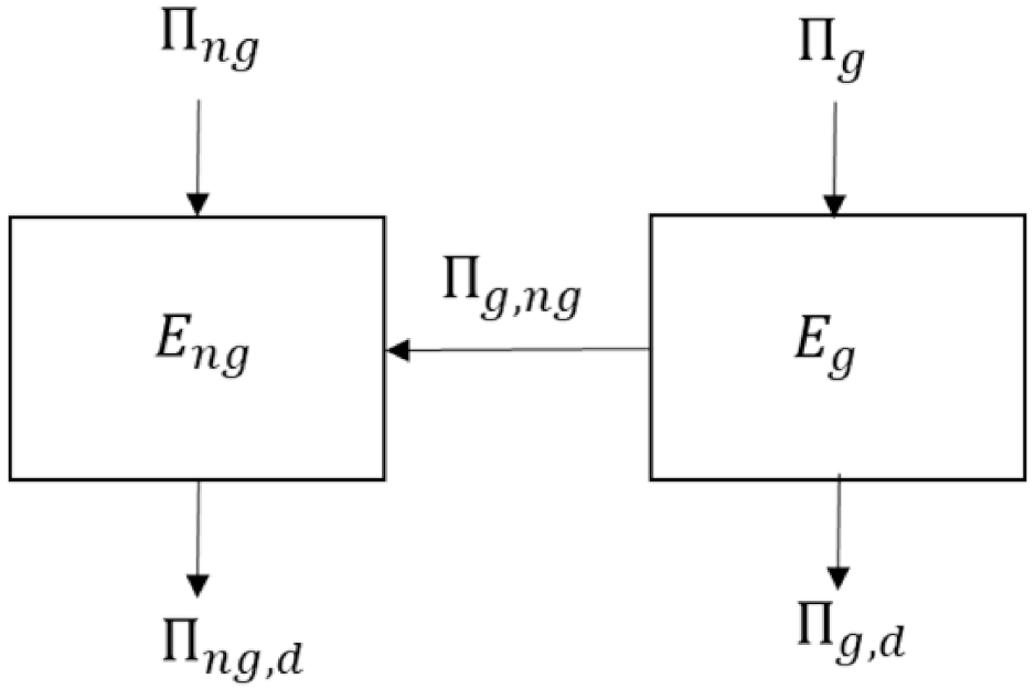
- Establish a general expression for the energy sound decay in a two-system SEA model.
- Express the total sound energy decay in the parameter sound strength as defined in ISO 3382-1.
- From the expression for the total sound energy decay, derive an expression for the speech clarity and the reverberation time .
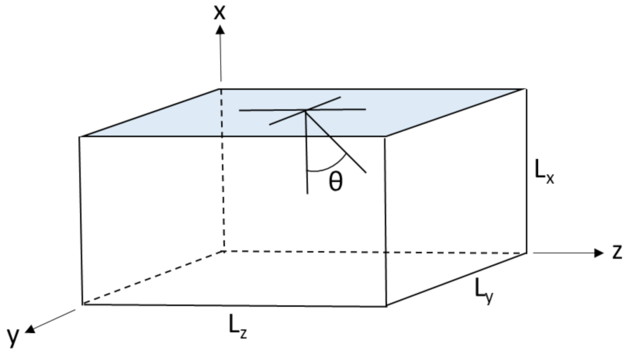
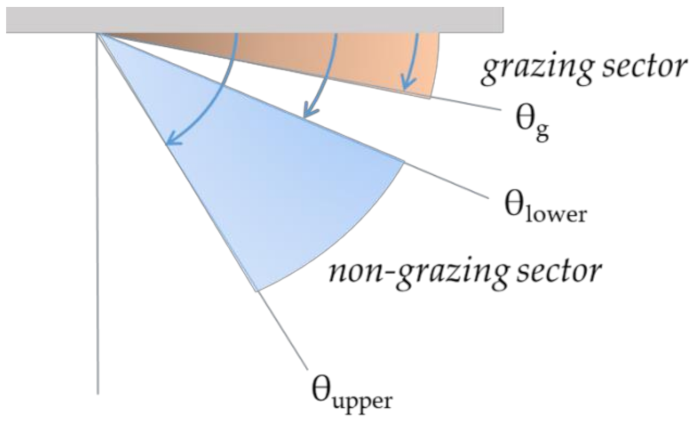
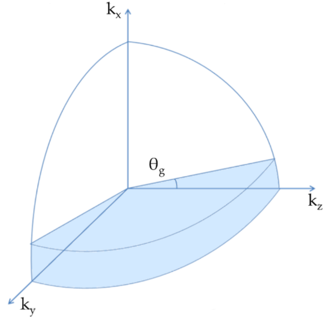
- Subdivide the total sound field into a grazing and non-grazing part where grazing refers to sound waves propagating almost parallel to the absorbent ceiling.
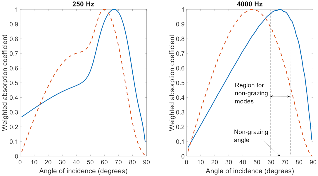
- Calculate the angle-dependent absorption coefficient, Section 3.2.1.
- Estimate the number of modes in the grazing subsystem as well as a representative absorption coefficient, Section 3.2.2.
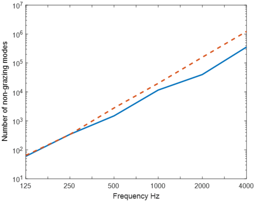
- Estimate the number of modes in the non-grazing subsystem as well as a representative absorption coefficient, Section 3.2.3. Two approaches for estimation of the number of non-grazing waves were used: one empirical and one theoretical.
- Based on a 2-dim and 3-dim reverberation formula, estimate the reverberation times and corresponding to the grazing and non-grazing subsystem, respectively. See Section 3.2.4.
- By knowing and and the number of modes in each subsystem, the energy ratio C for the grazing and non-grazing sound fields in the formula for sound strength can be calculated.
3. Theory
3.1. The SEA Model
3.2. Estimation of the Inherent Parameters , and
3.2.1. The Angle-Dependent Absorption Coefficient
3.2.2. Estimation of and
3.2.3. Estimation of and
3.2.4. Estimation of and
3.2.5. Estimation of
3.3. Summary
4. Measurements and Methods
4.1. Measurement Configurations
4.2. Measurement Method
4.3. Repeatability
4.4. Estimation of the Equivalent Scattering Absorption Area
4.5. Comparison between Measurements and Calculations
5. Results
5.1. Estimation of
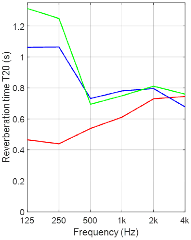
5.2. Measurement Results
6. Discussion
7. Conclusions
Author Contributions
Funding
Institutional Review Board Statement
Informed Consent Statement
Data Availability Statement
Acknowledgments
Conflicts of Interest
Appendix A
Appendix B
References
- ISO. ISO 3382-1: 2009, Acoustics—Measurement of Room Acoustic Parameters—Part 1: Performance Spaces; ISO: Geneva, Switzerland, 2009. [Google Scholar]
- ISO. ISO 3382-2: 2008, Acoustics—Measurement of Room Acoustic Parameters—Part 2: Reverberation Time in Ordinary Rooms; ISO: Geneva, Switzerland, 2008. [Google Scholar]
- Astolfi, A.; Pellerey, F. Subjective and objective assessment of acoustical and overall environmental quality in secondary school clas srooms. J. Acoust. Soc. Am. 2008, 123, 163–173. [Google Scholar] [CrossRef] [PubMed] [Green Version]
- Shield, B.; Conetta, R.; Dockrell, J.; Connolly, D.; Cox, T.; Mydlarz, C. A survey of acoustic conditions and noise levels in secondary school classrooms in England. J. Acoust. Soc. Am. 2015, 137, 177–188. [Google Scholar] [CrossRef]
- Shield, B.M.; Dockrell, J. The effects of environmentaland classroom noise on the academic attainments of primary school children. J. Acoust. Soc. Am. 2008, 123, 133–144. [Google Scholar] [CrossRef] [PubMed] [Green Version]
- Shield, B.M.; Dockrell, J. The effects of noise on children at school: A review. J. Build. Acoust. 2003, 10, 97–116. [Google Scholar] [CrossRef]
- Ljung, R.; Israelsson, K.; Hygge, S. Speech Intelligibility and Recall of Spoken Material Heard at Different Sig-nal-to-noise Ratios and the Role Played by Working Memory Capacity. Appl. Cogn. Psychol. 2013, 27, 198–203. [Google Scholar] [CrossRef]
- Yang, W.; Bradley, J.S. Effects of room acoustics on the intelligibility of speech in classrooms for young children. J. Acoust. Soc. Am. 2009, 125, 922–933. [Google Scholar] [CrossRef] [PubMed] [Green Version]
- Bradley, J.S.; Sato, H. The intelligibility of speech in elementary school classrooms. J. Acoust. Soc. Am. 2008, 123, 2078–2086. [Google Scholar] [CrossRef] [Green Version]
- Oberdörster, M.; Tiesler, G. Akustiche Ergonomie der Schule, Schriftenreihe der Bundesanstalt fur Arbeitsschutz und Arbeitsmedizin, Forshung Fb1071; Universität Bremen: Bremen, Germany, 2006. [Google Scholar]
- Sato, H.; Bradley, J.S. Evaluation of acoustical conditions for speech communication in working elementary school classrooms. J. Acoust. Soc. Am. 2008, 123, 2064–2077. [Google Scholar] [CrossRef] [Green Version]
- Lyberg-Åhlander, V.; Rydell, R.; Löfqvist, A. Speaker’s comfort in teaching environments: Voice problems in Swedish teaching staff. J. Voice 2011, 25, 430–440. [Google Scholar] [CrossRef]
- Pelegrin-Garcia, D.; Brunskog, J.; Lyberg-Åhlander, V.; Löfqvist, A. Measurement and prediction of voice supportand room gain in school classrooms. J. Acoust. Soc. Am. 2012, 131, 194–204. [Google Scholar] [CrossRef] [PubMed]
- Pelegrin-Garcia, D. Speakers’ comfort and voicelevel variationin classrooms: Laboratory research. J. Acoust. Soc. Am. 2012, 132, 249–260. [Google Scholar] [CrossRef]
- Bistrup, M. Health Effects of Noise on Children and the Perception of the Risk of Noise; National Institute of Public Health: Cpenhagen, Denmark, 2001. [Google Scholar]
- Bistrup, M. Children and Noise-Prevention of Adverse Effects; National Institute of Public Health: Cpenhagen, Denmark, 2002. [Google Scholar]
- Waye, K.P.; Fredriksson, S.; Hussain-Alkhateeb, L.; Gustafsson, J.; Van Kamp, I. Preschool teachers’ perspective on how high noise levels at preschool affect children’s behavior. PLoS ONE 2019, 14, e0214464. [Google Scholar] [CrossRef] [Green Version]
- Ryherd, E.E.; Persson Waye, K.; Ljungkvist, L. Characterizing noise and perceived work environment in a neurological intensive care unit. J. Acoust. Soc. Am. 2008, 123, 747–756. [Google Scholar] [CrossRef]
- Haapakangas, A.; Hongisto, V.; Eerola, M.; Kuusisto, T. Distraction distance and disturbance by noise—An analysis of 21 open-plan offices. J. Acoust. Soc. Am. 2017, 141, 127–136. [Google Scholar] [CrossRef]
- ISO. ISO 3382-3:2012 Acoustics—Measurement of Room Acoustic Parameters—Part 3: Open Plan offices; ISO: Geneva, Switzerland, 2012. [Google Scholar]
- ISO. ISO 22955:2021 Acoustics—Acoustic Quality of Open Office Spaces; ISO: Geneva, Switzerland, 2021. [Google Scholar]
- Bradley, J. Review of objective room acoustics measures and future needs. Appl. Acoust. 2011, 72, 713–720. [Google Scholar] [CrossRef]
- Sato, H.; Morimoto, M.; Sato, H.; Wada, M. Relationship between listening difficulty and acoustical objective measures in reverberant fields. J. Acoust. Soc. Am. 2008, 123, 2087–2093. [Google Scholar] [CrossRef] [Green Version]
- Harvie-Clark, J.; Dobinson, N.; Hinton, R. Acoustic Response in Non-Diffuse Rooms. In Proceedings of the Euronoise, Prague, Czech Republic, 10–13 June 2012. [Google Scholar]
- Rindel, J.H. Acoustical capacity as a means of noise control in eating establishment. In Proceedings of the Joint Baltic Nordic Acoustics Meeting, Odense, Denmark, 18–20 June 2012. [Google Scholar]
- Nijs, L.; Rychtáriková, M. Calculating the optimum reverberation time and absorption coefficient for good speech intelligibility in classroom design using U50. Acta Acust. United Acust. 2011, 97, 93–102. [Google Scholar] [CrossRef]
- Barron, M.; Lee, L.J. Energy relations in concert auditoriums. I. J. Acoust. Soc. Am. 1988, 84, 618–628. [Google Scholar] [CrossRef]
- Barron, M. Theory and measurement of early, late and total sound levels in rooms. J. Acoust. Soc. Am. 2015, 137, 3087–3098. [Google Scholar] [CrossRef] [PubMed]
- Nilsson, E. Input data for acoustical design calculations for ordinary public rooms. In Proceedings of the 24th International Congress on Sound and Vibration, London, UK, 23–27 July 2017. [Google Scholar]
- Sabine, W.C. Collected Papers on Acoustics; Dover Publications: New York, NY, USA, 1964. [Google Scholar]
- Rasmussen, B.; Brunskog, J.; Hoffmeyer, D. Reverberation time in class rooms—Comparison of regulations and classi-fication criteria in the Nordic countries. In Proceedings of the Joint Baltic—Nordic Acoustics Meeting, Odense, Denmark, 18–20 June 2012. [Google Scholar]
- IEC. IEC 60268-16 Sound System Equipment—Part 16: Objective Rating of Speech Intelligibility by Speech Transmission Index; IEC: Geneva, Switzerland, 2011. [Google Scholar]
- Astolfi, A.; Parati, L.; D’Orazio, D.; Garai, M. The new Italien standard UNI 11532 on acoustics for schools. In Proceedings of the 23rd International Congress on Acoustics, Aachen, Germany, 9–13 September 2019. [Google Scholar]
- Cremer, L.; Muller, H.A.; Schultz, T.J. Principles and Applications of Room Acoustics Vol 1; Applied Science Publishers: London, UK, 1982. [Google Scholar]
- Kuttruff, H. Room Acoustics, 3rd ed.; Elsevier Science Publishers Ltd.: London, UK, 1991. [Google Scholar]
- Joyce, W.B. Sabine’s reverberation time and ergodic auditoriums. J. Acoust. Soc. Am. 1975, 58, 643–655. [Google Scholar] [CrossRef]
- Joyce, W.B. Exact effect of surface roughness on the reverberation time of a uniformly absorbing spherical enclosure. J. Acoust. Soc. Am. 1978, 64, 1429–1436. [Google Scholar] [CrossRef]
- Fitzroy, D. Reverberation formulae which seem to be more accurate with non-uniform distribution of absorption. J. Acoust. Soc. Am. 1959, 31, 893–897. [Google Scholar] [CrossRef]
- Neubauer, N.O. Estimation of reverberation time in rectangular rooms with non-uniformly distributed absorption using a modified Fitzroy equation. Build. Acoust. 2001, 8, 115–137. [Google Scholar] [CrossRef]
- Arau-Puchades, H. An improved reverberation formula. Acustica 1988, 65, 163–180. [Google Scholar]
- Cucharero, J.; Hänninen, T.; Lokki, T. Influence of sound-absorbing material placement on room acoustical parame-ters. Acoustics 2019, 1, 644–660. [Google Scholar]
- Sakuma, T. Approximate theory of reverberation in rectangular rooms with specular and diffuse reflections. J. Acoust. Soc. Am. 2012, 132, 2325–2336. [Google Scholar] [CrossRef] [PubMed]
- Bistafa, S.R.; Bradley, J.S. Predicting reverberation times in a simulated classroom. J. Acoust. Soc. Am. 2000, 108, 1721–1731. [Google Scholar] [CrossRef] [Green Version]
- Prodi, N.; Visentin, C. An experimental evaluation of the impact of scattering on sound field diffusivity. J. Acoust. Soc. Am. 2013, 133, 810–820. [Google Scholar] [CrossRef] [PubMed]
- ISO. ISO 354:2003 Acoustics—Measurement of Sound Absorption in a Reverberation Room; ISO: Geneva, Switzerland, 2003. [Google Scholar]
- Nolan, M.; Berzborn, M.; Fernandez-Grande, E. Isotropy in decaying reverberant sound fields. J. Acoust. Soc. Am. 2020, 148, 1077–1088. [Google Scholar] [CrossRef]
- Nilsson, E. Decay Processes in Rooms with Non-Diffuse Sound Fields Part I: Ceiling Treatment with Absorbing Material. Build. Acoust. 2004, 11, 39–60. [Google Scholar] [CrossRef]
- Nilsson, E. Decay processes in rooms with non-diffuse sound fields—Part II: Effect of irregularities. Build. Acoust. 2004, 11, 133–143. [Google Scholar] [CrossRef]
- EN 12354-6:2004, Building Acoustics—Estimation of Acoustic Performance of Buildings from the Performance of Elements—Part 6: Sound Absorption in Enclosed Spaces; CEN: Brussels, Belgium, 2004.
- Lochner, J.; Burger, J. The influence of reflections on auditorium acoustics. J. Sound Vib. 1964, 1, 426–454. [Google Scholar] [CrossRef]
- Visentin, C.; Pellegatti, M.; Prodi, N. Effect of a single lateral diffuse reflection on spatial percepts and speech intelligi-bility. J. Acoust. Soc. Am. 2020, 148, 122–140. [Google Scholar] [CrossRef]
- Bradley, J.S.; Sato, H.; Picard, M. On the importance of early reflections for speech in rooms. J. Acoust. Soc. Am. 2003, 113, 3233–3244. [Google Scholar] [CrossRef] [Green Version]
- Lyon, R.H.; De Jong, R.G. Theory and Application of Statistical Energy Analysis, 2nd ed.; RH Lyon Corp: Cambridge, MA, USA, 1998; p. 02138. [Google Scholar]
- Crighton, D.G.; Dowling, A.P.; Ffowcs Williams, J.E.; Heckl, M.; Leppington, F.G. Modern Methods in Analytical Acoustics; Springer London: London, UK, 1992; Chapter 8. [Google Scholar]
- Nilsson, E. Decay Processes in Rooms with Non-Diffuse Sound Fields; Report TVBA-1004; Engineering Acoustics, LTH, Lund University: Lund, Sverige, 1992. [Google Scholar]
- Barron, M.; Barron, M. Growth and decay of sound intensity in rooms according to some formulae of geometric acoustics theory. J. Sound Vib. 1973, 27, 183–196. [Google Scholar] [CrossRef]
- Available online: https://alphacell.matelys.com/ (accessed on 16 July 2021).
- Available online: https://norsonic.se/product_single/norflag/ (accessed on 16 July 2021).
- Miki, Y. Acoustical properties of porous materials. Modifications of Delany-Bazley models. J. Acoust. Soc. Jpn. (E) 1990, 11, 19–24. [Google Scholar] [CrossRef]
- Jeong, C.-H. Guidline for adopting the local reaction assumption for porous absorbers in terms of random incidence ab-sorption coefficients. Acta Acoust. United Acust. 2011, 97, 779–790. [Google Scholar] [CrossRef]
- Delany, M.; Bazley, E. Acoustical properties of fibrous absorbent materials. Appl. Acoust. 1970, 3, 105–116. [Google Scholar] [CrossRef]
- Komatsu, T. Improvement of the Delaney-Bazley and Miki models for fibrous sound-absorbing materials. Acoust. Sci. Tech. 2008, 29, 121–129. [Google Scholar] [CrossRef] [Green Version]
- Paris, E.T. On the coefficient of sound-absorption measured by the reverberation method. Philos. Mag. 1928, 5, 489. [Google Scholar] [CrossRef]
- Bakoulas, K. Optimization of an Energy-Based Room Acoustics Model that Considers Scattering and Non-Uniform Absorption. Master’s Thesis, Department of Electrical Engineering, Technical University of Denmark, Lyngby, Denmark, 2017. [Google Scholar]
- Nilsson, E. Sound scattering in rooms with ceiling treatment. In Nordtest Technical Report TR 606; Nordic Innovation Centre: Oslo, Norway, 2007. [Google Scholar]
- ISO. ISO 11654:1997 Acoustics—Sound Absorbers for Use in Buildings—Rating of Sound Absorption; ISO: Geneva, Switzerland, 1997. [Google Scholar]
- Arvidsson, E.; Nilsson, E.; Hagberg, D.B.; Karlsson, O.J.I. The effect on room acoustical parameters using a combina-tions of absorbers and diffusors—An experimental study in a classroom. Acoustics 2020, 2, 505–523. [Google Scholar] [CrossRef]
- Marbjerg, G.; Brunskog, J.; Jeong, C.-H.; Nilsson, E. Development and validation of a combined phased acoustical radi-osity and image source model for predicting sound fields in rooms. J. Acoust. Soc. Am. 2015, 138, 1457–1468. [Google Scholar] [CrossRef] [PubMed]
- Pind, F.; Jeong, C.-H.; Engsig-Karup, A.P.; Hesthaven, J.S.; Stromann-Andersen, J. Time-domain room acoustic simula-tions with extended-reacting porous absorbers using the discontinuous Galerkin method. J. Acoust. Soc. Am. 2020, 148, 2851–2863. [Google Scholar] [CrossRef] [PubMed]
- Cremer, L.; Muller, H.A.; Shultz, T.J. Principles and Applications of Room Acoustics Vol 2; Applied Science Publishers: London, UK, 1982. [Google Scholar]
- Morse, P.M.; Bolt, R.H. Sound waves in rooms. Rev. Mod. Phys. 1944, 16, 69–150. [Google Scholar] [CrossRef]


| Frequency Hz | 125 | 250 | 500 | 1000 | 2000 | 4000 |
| 0.63 | 0.31 | 0.14 | 0.17 | 0.07 | 0.08 |
| Case | Ceiling and Wall Panels | Mounting Height (Depth of Air Cavity) of Suspended Ceiling (mm) | Air Flow Resistivity of Ceiling Absorber (kPas/m2) |
|---|---|---|---|
| 1 | 50 mm glasswool ceiling absorber * no wall panels | 750 | 11.8 |
| 2 | 15 mm glasswool ceiling absorber **, no wall panels | 785 | 77.8 |
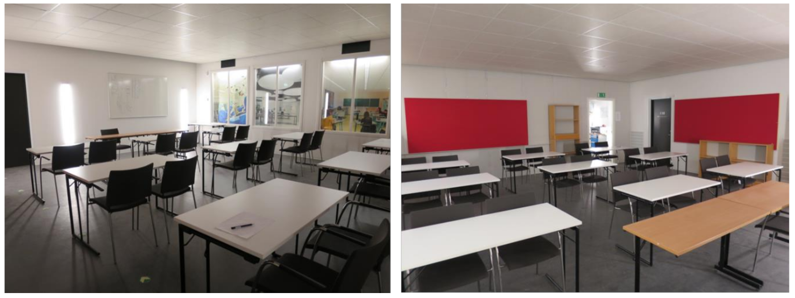
| 3 | 15 mm glasswool ceiling absorber **, 6.48 m2 40 mm glasswool wall absorber *** distributed on two adjacent walls and directly mounted on the walls, see Figure 7. | 785 | NA |
| 4 | 15 mm glasswool ceiling absorber ** | 185 | 77.8 |
| 5 | 50 mm glasswool ceiling absorber * | 150 | 11.8 |
| 125 Hz | ±0.61 | ±0.56 | ±0.077 |
| 250 Hz | ±0.30 | ±0.29 | ±0.018 |
| 500 Hz | ±0.40 | ±0.29 | ±0.010 |
| 1000 Hz | ±0.25 | ±0.27 | ±0.006 |
| 2000 Hz | ±0.37 | ±0.38 | ±0.010 |
| 4000 Hz | ±0.36 | ±0.36 | ±0.008 |
Publisher’s Note: MDPI stays neutral with regard to jurisdictional claims in published maps and institutional affiliations. |
© 2021 by the authors. Licensee MDPI, Basel, Switzerland. This article is an open access article distributed under the terms and conditions of the Creative Commons Attribution (CC BY) license (https://creativecommons.org/licenses/by/4.0/).
Share and Cite
Nilsson, E.; Arvidsson, E. An Energy Model for the Calculation of Room Acoustic Parameters in Rectangular Rooms with Absorbent Ceilings. Appl. Sci. 2021, 11, 6607. https://doi.org/10.3390/app11146607
Nilsson E, Arvidsson E. An Energy Model for the Calculation of Room Acoustic Parameters in Rectangular Rooms with Absorbent Ceilings. Applied Sciences. 2021; 11(14):6607. https://doi.org/10.3390/app11146607
Chicago/Turabian StyleNilsson, Erling, and Emma Arvidsson. 2021. "An Energy Model for the Calculation of Room Acoustic Parameters in Rectangular Rooms with Absorbent Ceilings" Applied Sciences 11, no. 14: 6607. https://doi.org/10.3390/app11146607
APA StyleNilsson, E., & Arvidsson, E. (2021). An Energy Model for the Calculation of Room Acoustic Parameters in Rectangular Rooms with Absorbent Ceilings. Applied Sciences, 11(14), 6607. https://doi.org/10.3390/app11146607