Article

Challenges and Accomplishments in Mechanical Testing Instrumented by In Situ Techniques: Infrared Thermography, Digital Image Correlation, and Acoustic Emission

by
Aleksander Sendrowicz
*,
Aleksander Omholt Myhre
*,
Seweryn Witold Wierdak
and
Alexei Vinogradov
Department of Mechanical and Industrial Engineering, Norwegian University of Science and Technology—NTNU, 7034 Trondheim, Norway
*
Authors to whom correspondence should be addressed.
Appl. Sci. 2021, 11(15), 6718; https://doi.org/10.3390/app11156718
Submission received: 25 June 2021 / Revised: 15 July 2021 / Accepted: 20 July 2021 / Published: 22 July 2021

Abstract

:

Featured Application

The proposed research is applicable to advanced laboratory mechanical testing in academic or research settings, and it is supposed be applied to the development of novel means for non-destructive testing and condition monitoring in industry.

Abstract

A current trend in mechanical testing technologies is to equip researchers and industrial practitioners with the facilities for non-destructive characterisation of the deformation and fracture processes occurring on different scales. The synergistic effect of such a combination of destructive and non-destructive techniques both widens and deepens existing knowledge in the field of plasticity and fracture of materials and provides the feedback sought to develop new non-destructive testing approaches and in situ monitoring techniques with enhanced reliability, accuracy and a wider scope of applications. The macroscopic standardised mechanical testing is still dominant in the research laboratories and industrial sector worldwide. The present paper reviews multiple challenges commonly faced by experimentalists, aiming at enhancing the capability of conventional mechanical testing by a combination of contemporary infrared thermography (IRT), rapid video imaging (RVI) with non-contact strain mapping possibilities enabled by the digital image correlation (DIC) method, and the acoustic emission (AE) technique providing unbeatable temporal resolution of the stochastic defect dynamics under load. Practical recommendations to address these challenges are outlined. A versatile experimental setup uniting the unique competencies of all named techniques is described alone with the fascinating possibilities it offers for the comprehensive characterisation of damage accumulation during plastic deformation and fracture of materials. The developed toolbox comprising practical hardware and software solutions brings together measuring technologies, data, and processing in a single place. The proposed methodology focuses on the characterisation of the thermodynamics, kinematics and dynamics of the deformation and fracture processes occurring on different spatial and temporal scales. The capacity of the proposed combination is illustrated using preliminary results on the tensile and fatigue behaviour of the fcc Inconel-625 alloy used as a representative example. Dissipative processes occurring in this alloy are assessed through the complex interplay between the released heat, acoustic emission waves, and expended and stored elastic energy.

1. Introduction

Traditionally, the primary mechanical properties of structural materials are obtained through tensile or cyclic testing. Departing from routine mechanical testing procedures is required whenever the deformation and fracture processes have to be assessed and understood. A wealth of contemporary highly sensitive non-destructive experimental methods has emerged recently to meet these challenges and to combine the advantages of both precise mechanical testing and in situ characterisation of underlying mechanisms in pseudo-real time scale. The modern high resolution infrared thermography (IRT), rapid video imaging (RVI), digital image correlation (DIC), and acoustic emission (AE) techniques are those to be listed first among many others. Although infrared methods are unique in that they provide direct access to the thermodynamics of plastic flow, strain localisation and fracture, AE offers an unbeatable temporal resolution of characterising rapid dynamics of stress relaxation processes occurring under load. Thus, both these methods reflecting the elastic energy dissipation in solids (albeit in different ways) are complementary to each other. RVI allows to inspect the development of deformation at a micro-second temporal resolution, and a combination with DIC results in the assessment of the deformation and cyclic behaviour of the material.
IRT is a versatile method in materials testing [1]. The traditional application domain of IRT is the non-contact stress analysis, which bears its origin in the thermoelastic effect in materials [2,3,4,5]. Under adiabatic conditions, the analysis of the thermoelastic effects provides a direct link between temperature variations and hydrostatic stress variation pattern [6]. In more complex settings, scattering in the infrared imaging can serve as a measure of strain energy fluctuations in the vicinity of the fatigue crack tip, thus, providing the possibility to characterise the J-integral or the stress intensity factor K during fatigue crack growth [7] from non-contact thermographic measurements [8]. Amongst other appealing applications of IRT, the possibility proposed by Risitano to estimate the fatigue limit rapidly with a small number of samples is to be mentioned [9]. The further elaboration of this approach allowed not only the fatigue limit to be estimated, but the entire fatigue life curve to be recovered in a cost-effective way [10]. Another common use of the IRT method relies on the comparison of the temperature response with the load signal. If the adiabatic conditions are met and no cyclic plastic deformation occurs, the temperature change should be proportional to the change in the load signal (with a negative proportionality constant). This behaviour changes when plasticity is present [7]. Being a dissipative process by nature, plastic deformation affects the temperature response. Based on this premise, Ancona et al. [11] used a second order Fourier series to investigate the first- and second-order harmonics of the temperature, which allows to perform thermoelastic stress analysis, locate the crack tip, and gain information regarding plastic deformation. Other authors have focused on the energy sources that cause the dissipation of the thermal energy at the crack tip, and its relation to damage [12]. Many of these analytical approaches can be combined into a common workflow.
RVI has been proven to be a technique enabling direct assessment of the dynamic effects related to plastic deformation and fracture observable at the surface. The rapid observation of the deformation-induced surface morphology permits for the in-depth characterisation of the failure mechanisms occurring at time scales ranging broadly from seconds to micro-seconds. For instance, Ju et al. [13] investigated the effect of the crack velocity in the vicinity of the crack tip, which has not been well understood as yet. The challenges faced frequently by the RVI users include, but are not limited to, (i) adequate illumination, which is particularly important for high shutter speeds; (ii) limited recording time [14]; and (iii) duration of an event, which can be too short to be captured with sufficient resolution [15]. These commonly known issues highlight the significance of an automated triggering system allowing to capture only the moments of interest with a proper reference to external conditions such as load, strain, temperature, etc. The successful attempt to use the acoustic emission technique to trigger the rapid video camera in a mechanical testing setup has been reported in [16].
DIC is a modern non-contact method of local displacement measurements which is gaining greater and greater popularity due to its versatility and high accuracy results of the measurement of the strain tensor components [1], which is comparable to or exceeds that of other conservative methods available to researchers [17]. The DIC technique enables the full-field displacement and strain maps to be obtained in a set of photographs taken at different stages of deformation by tracking unique features in the images. DIC is an undemanding method that uses a simple set-up permitting for a widely variable sensitivity and resolution, and for high automation of displacement and strain measurements [15]. The report by Gao et al. [15] is one of multiple examples of the extensive use of RVI in conjunction with DIC to obtain displacement and strain fields, as well as to estimate the strain distribution in the vicinity of the crack tip, and the size of the plastic zone. The outstanding sub-micrometre (per pixel) resolution has been achieved with the DIC method in [18], where the plastic strain field was studied near a growing fatigue crack in a nickel-based superalloy. Pan et al. [19] provided a detailed analysis of the DIC measurement accuracy, considering the influence of both experimental conditions and the correlation algorithm itself. The guidelines for achieving high accuracy strain mapping have been provided too. Many of those recommendations were taken into consideration and implemented in the present work.
Both DIC and IRT methods are capable of characterising the local deformation behaviour of materials by full-field measurements, albeit in remarkably different ways as they refer to different physical properties. However, they both have advantages and disadvantages, which have been well understood and documented in abundant literature (for details, interested readers are referred to comprehensive reviews [1,19,20]). A qualitative side-by-side comparison of DIC and IRT techniques was made in [21], where aluminium specimens were subjected to 3-point bending loading with different velocities. It was shown that both methods were capable of visualising a plastic zone quite well, i.e., the region where heat generated occurred during plastic deformation was comparable to the plastic zone determined by DIC. However, the performance of both methods differed dramatically in dependence on the strain rate: the DIC performed notably better under quasi-static conditions, while IRT revealed the plastic zone much better under dynamic loading. Despite good visible agreement between IRT and DIC images, temperature distributions cannot be mapped directly to strain distributions since both methods are footed on fundamentally different principles, and refer to physically different measured quantities—displacements and temperature, respectively.
An AE technique reflecting the rapid local stress relaxation processes in solids has long been acknowledged by materials scientists as a powerful tool enabling the assessment of the dynamic behaviour of defects in real time scale, and the in situ characterisation of the deformation and fracture processes under load [22]. The method has gained popularity due to its extraordinarily high sensitivity to elementary mechanisms of plastic deformation—dislocation slip [23,24,25], mechanical twinning [26,27,28,29,30], temperature- or deformation-induced phase transformations [31,32,33,34,35], plastic instabilities of various kinds [36,37,38,39,40,41,42,43,44], and, of course, cracks of various types. Robust discrimination between different potential sources of AE signals is an everlasting and extremely challenging problem in the AE field. The feasibility of using various classifiers and signal- or pattern-recognition techniques to establish a basis for reliable distinguishing between different AE sources and background noise in the same dataset has been demonstrated on many materials, and several classifiers differing by classification methods, features, cost functions, robustness, etc., have been proposed and tested in the past (see, e.g., [45,46,47,48]). The method proposed by Pomponi and Vinogradov [49]) is incorporated in the present setup as a tool of choice, as will be discussed in the next section. The acoustic emission elastic waves emitted at the source and propagated towards the sensor fall in the ultrasonic frequency range, and, consequently, the AE method requires high-speed acquisition of broadband waveforms at 1–20 Msamples/s. Continuous data streaming with high acquisition rate is resource-demanding, and particularly challenging in long-term applications, e.g., during fatigue testing. The specific details of the application of AE to the fatigue crack growth monitoring will be reviewed below.
Thus, the combination of the named techniques provides a rich source of detailed information about thermodynamics, kinematics, and dynamics of deformation and fracture processes occurring on different scales. As stated above, each technique is unique, adapted to a specific purpose, and different from others in its own regard. Although the advantages of all constituent techniques are accumulated in a combined setup, individual disadvantages can be mitigated (if not avoided altogether). The major asset of the IRT technique is that it provides integral, direct access to thermodynamic aspects of plastic deformation and fracture on the macro-scale through the measurements of the local distribution of temperature on the surface—information that is not accessible otherwise. The RVI system clarifies the details of the occurrence of deformation and fracture mechanisms, which are reflected by the surface relief on the scale ranging from macro (a whole specimen) to micro (grain, sub-grain, individual slip lines, deformation twins, microcracks, etc.), depending on the lens used. When powered by DIC, it quantifies the local strain and stress distribution in the region of interest (ROI).
Recognition of unique benefits offered by a combination of these methods has prompted several researchers to implement them in a single experimental setup and explore new possibilities for monotonic and fatigue testing of different structural materials—aluminium alloys [50,51,52], titanium alloys [50], 316 austenitic stainless steel [53,54], magnesium alloy AZ31 [55], various composites [6,56], concrete [57], and rock [58].
It is known that, while the combination of IRT, AE, and RVI/DIC is a powerful approach, offering a quite unique and comprehensive piece of information regarding various aspects of the deformation and fracture of the testing material, this novel approach poses many challenges faced by laboratory practitioners worldwide. The burgeoning interest and the increasing number of publications exploiting the named techniques in various combinations motivated us to review the existing challenges and good practices to address them based on our first-hand experience. The main challenges to be addressed include: (i) high mechanical noise from the dynamic testing frames affecting AE measurements, (ii) electrical noise and interference between all the devices used in the setup influencing the measured AE signal, (iii) flexible synchronisation of all testing and measuring devices, (iv) movement of the specimen and the region of interest away from the camera’s field of view, (v) combination of IRT and DIC images in the common data processing framework, (vi) finding the crack tip position by means of both IRT and DIC, (vii) correcting the thermal measurements for the lower than unity infrared emissivity, (viii) processing of noisy IRT information to calculate the heat dissipation from weak sources, etc. In what follows, we propose a versatile experimental setup addressing the named major and a few other minor (yet frequently faced and annoying) hardware and software challenges, thus enabling the seamless and synchronous operation of the IRT, AE, and RVI/DIC techniques, and report the preliminary results on the characterisation of plastic deformation and fatigue crack growth in the commercial Inconel-625 alloy.

2. Methods and Materials

2.1. Theoretical Background for Data Processing

The fundamentals of DIC, and thermodynamic calculations are briefly explained in Section 2.1.1 and Section 2.1.2, respectively, and this theory is further used in the final calculations.

2.1.1. Continuum Mechanics and Digital Image Correlation Measurements

The digital image correlation technique combines image recording by optical cameras and software tracking procedures for accurate measurements of changes occurring in images due to deformation. Full-field displacement and strain maps are obtained by comparing surface images acquired along the deformation path. The algorithm recognises unique surface features and allocates their coordinates to the image pixels. It then tracks the relative displacement of these features in a set of sequentially obtained images and compares it to the first reference image, which often represents the undeformed state. The tracking is based on the iterative optimisation of a deformation vector to achieve a high correlation between the pairs of images. Thus, a stochastic, high contrast pattern on the surface throughout the entire test is required for the DIC method to find unique correlations. This can be obtained by painting the surface of the specimen with a speckle pattern. However, in many cases, the natural surface morphology inherited from the specimen preparation, e.g., grinding, is sufficient for a successful analysis [59]. The DIC analysis returns a field of displacements u expressed in coordinates corresponding to either reference X or deformed configuration x . Displacements are used to find the deformation gradient F , which is a second-order tensor defined as
F = x X = I + u X
containing information about both the stretch and rotation of the body. Here I is the identity matrix, and denotes the partial differential. F is commonly used in calculations of virtually any type of strain defined in continuum mechanics.
For elastic energy (or power) density calculations, stresses and strains must be energetically conjugate. For the Cauchy stress tensor σ , its energetic conjugate is the deformation rate tensor D , which, in turn, is calculated from the velocity gradient L as
D = 1 2 ( L · L T )
The velocity gradient is defined as the spatial derivative of the velocity v with respect to coordinates in the deformed configuration x
L = v x
Tracking the velocity of a given point in the deformed configuration must account for that the point moves with strain or time. To simplify calculations, the velocity gradient L can be obtained from the deformation gradient F expressed in the reference configuration according to Equation (4). The data given in the reference configuration make it easy to track a point of interest at large deformations and displacements.
L = F ˙ · F 1
When the Cauchy stress tensor and the deformation rate tensor are known, the mechanical power density can be calculated as
p M = σ : D

2.1.2. Heat Equation and Infrared Thermography

The origin and theory of IRT has been described in detail elsewhere [60,61]. For the sake of completeness, the fundamentals of IRT-based methods are briefly described below.
In the thermographic systems, equilibrium infrared radiation emitted by a body is detected in a non-contact way by an infrared detector. Assuming a black-body model and using Stefan–Boltzmann’s law, the temperature of the solid is obtained. When the test object does not satisfy the black body assumption, its emissivity must be considered and accounted for. The infrared emissivity is a function of wavelength, but a IRT camera works in the spectral range where it does not distinguish between wavenumbers. To correct for the non-unit emissivity, a grey body model can be adopted under the assumption that the emissivity is uniformly distributed within the camera’s spectral bandpass. Since metals are opaque, the in-band radiance (IBR) received by the camera’s sensor can be divided into three part: (i) the radiance emitted by the object surface, (ii) the radiance reflected from the object, and (iii) the radiance emitted by the atmosphere. The last term is often negligible when the distance between the lens and the object is small, while the remaining terms can be approximated as
L m ε b o d y ¯ × L P l ( T b o d y ) + [ 1 ε b o d y ¯ ] × L P l ( T s )
where L m is the IBR measured by the system, L P l ( T ) is the IBR of the Planck’s function at temperature T, ε b o d y ¯ is the average emissivity in the operating spectrum, T b o d y , and T s are the temperatures of the object of interest and surroundings, respectively. This equation assumes that the radiance emitted from the object and the surroundings, is represented by Planck’s law. The IBR is an integral of radiation over the working spectrum of the camera-lens system. Rearranging these terms gives the following equation
L P l ( T b o d y ) L m [ 1 ε b o d y ¯ ] × L P l ( T s ) ε b o d y ¯
which allows calculating the black body equivalent IBR of the test object. From the last equation, the temperature of the object can be calculated since L P l ( T ) is a bijective function connecting the radiometric temperature to IBR (for further information, interested readers are referred to [62]).
According to Fourier’s law, the differential heat conduction equation for anisotropic materials takes a form
ϕ q = k T
where Heat flux ϕ q denotes the heat flux vector (the flow of heat through a unit area per unit of time), k is the coefficient of heat conductivity, which, in general, can be expressed in a symmetric tensorial form, and T stands for the temperature gradient. Applying this equation to the experimentally measured temperature field permits determining the heat flux. Equation (8) is sufficient to describe heat conduction under stationary conditions, i.e., when the temperature distribution across the solid and the heat flux remain constant in time. To account for the non-steady behaviour, a second independent equation is required. The energy conservation law is commonly used for this purpose in the form of the continuity equation [61]:
δ Q δ t = c p ρ T t
where the change in the internal heat energy with time, i.e., the heat power, is denoted as δ Q δ t (the symbol δ here, and in what follows, highlights that the infinitesimally small increment of heat is not a perfect differential), and it is related to the rate of the temperature change, c p is the specific heat capacity, and ρ is the material’s mass density. Conservation of energy implies that the accumulation of the thermal energy at a given point of the specimen volume is equal to the negative spatial derivative of heat flow at that point, plus any other energy put into the system. Combination of these equations gives the familiar heat conduction equation:
ρ c p T t = q ˙ + k 2 T
The term on the left-hand side is the change in the internal heat energy, q ˙ represents a heat source function that comprises contributions from a variety of existing heat sources or sinks, and the last term on the right-hand side describes the heat energy change due to the heat flow. The term q ˙ accounts for a wealth of contributors to the energy change (except conduction), such as radiative loss, heat convection on a surface, heat dissipation due to plastic work, thermoelastic effect, and, possibly, other mechanisms that can be involved in a specific case.
When applying Equation (10) to metals undergoing deformation, heat conduction is usually significantly larger than radiative loss, or convection [63] which can often be neglected. In the case of a large temperature difference between the metal and its surroundings, the heat loss due to these terms can be accounted for if necessary. Once these terms are neglected or accounted for, the remaining part of q ˙ will consist of the thermoelastic contribution, and the part of mechanical power dissipated as heat p D . The thermoelastic effect occurs as a reversible temperature change caused by the change in the first stress invariant s, and is usually described by the linear equation for the infinitesimally small increment of T as
d T = K t T d s
The thermoelastic parameter K t is usually assumed to be constant [64] and expressed as
K t = α T ρ c p
where α T is the coefficient of the linear thermal expansion, c p is the specific heat capacity (at constant pressure), and ρ is the materials density.
An integral of p D with respect to time gives the energy density dissipated as heat w D . The same applies to p M from Equation (5)—the time integral of p M yields the mechanical work (per unit volume) w M expended on the deformation. Both the heat energy dissipated by the system w D and the mechanical work w M enter the first law of thermodynamics, which relates these two quantities to the change in the stored energy density w S as
d w S = δ w M δ w D

2.2. Experimental Setup

Using the same design philosophy, two slightly different experimental setups have been developed for the axial monotonic and cyclic testing under load or displacement control and for fatigue crack growth (FCG) tests. The schematics of both setups are shown in Figure 1. Since the involved key techniques are essentially the same in both arrangements, the tensile setup can be considered as a simplified version of the one for FCG.
In addition to the testing machine and the three independent measurement systems representing IRT, AE, and RVI/DIC techniques, the entire setup does, however, require additional instrumentation and preparation to turn it working as desired. Specifically, depending on the testing machine and the grips, measures to reduce the machine noise, which is particularly severe on most commercially available servo-hydraulic frames, is required for the AE acquisition. The AE unit often needs to be galvanically isolated from all other devices to eliminate electrical interference and improve the signal-to-noise ratio (SNR): the sensors with conductive contact surfaces have to be isolated from the specimen, and triggering circuits have to be designed with optical decoupling of all signal connections. In the setup used in the present work, the high-speed CMOS-based camera PHOTRON SA-Z maintaining a square aspect ratio of 1024 × 1024 pixels for frame rates up to 20,000 fps (up to 1,000,000 fps at a reduced resolution) with 64 GB on-board memory was used. A versatile modular microscopic and microscopic long-focal zoom lens Navitar-6000 with the through-the-lens coaxial high-power Hayashi LA HDF7010RL LED illumination unit was attached to the camera for high-speed shooting. The maximal spatial resolution with this lens system is approximately 0.7 μm. The camera was mounted on a motorised computer-controlled linear stage LNR502E (Thorlabs, Newton, NJ, USA), which allows the camera to move together with the crack tip to measure the crack length precisely even when the surface is polished, and the camera’s position and relative motion would be difficult to track.
IRT measurements were performed using a Telops FAST M350 mid-wave, high-speed camera, with an operating spectral range of 1.5 μm to 5.4 μm and the indium antimonide (InSb) cooled sensor. The camera has a typical in the class noise equivalent temperature difference (NETD) value of 20 m K (referring to 30 ° C background temperature). Even though, NETD is a quantity that might characterise the inherent property of the sensor at a given reference temperature, when it comes to practical measurements, the NETD parameter represents the upper bound estimate of the thermal resolution of the entire thermographic system. The NETD value depends on the settings, most notably on the temperature of the tested object, the spectral transmittance of the camera optics, f-number characterising the lens aperture (a low f-number means a larger aperture), exposure time, etc. [65,66]. Therefore, the actual NETD value of the experimental setup can be considerably higher. The sensor has a 640 × 512 pixels resolution and the maximum frame rate is 355 fps at full resolution. The internal memory of the camera was 16 GB and a CameraLink interface enabling direct data transfer to an external drive. The camera was firmly mounted on a tripod as shown in Figure 1c. The IRC-LENS-G1-MW 1X microscopic lens (f/3) with a working distance of 260 mm was used in the FCG setup. The sensor size is 15 μm, which, in combination with the 1X lens, renders a spatial resolution of 15 μm. The Janos Technology 40,494 25 mm lens (f/2.3) with 1/4 extension ring was used in the axial setup, although both lens sets can be used interchangeably, depending on the dimensions of the test specimens.
For AE recording, the PC-controlled system based on 18 bits PCI-2 (MISTRAS, Princeton, NJ, USA) data acquisition board with a data streaming capability (see [67] for technical details) was used. The signal from the sensor output is amplified by 60 dB by the low-noise wide-band preamplifier 2/4/6 with the built-in band-pass 30–1200 kHz filter. The background noise level measured peak-to-peak was of 32 μV or less at the sensor output (depending on the sensor used). The MISTRAS F50α 200–800 kHz wideband sensor was used. Molykote 33 silicone-based grease was used as the coupling medium, and the sensor was mounted using a 3D-printed polymeric mechanical clamp. The background noise level at the sensor output was measured with the specimen mounted at zero load as of 3 μV rms (of 31 μV peak-to-peak) in the tensile setup and of 2.6 μV rms (of 27 μV peak-to-peak) in the FCG setup. The AE recording was performed continuously at 2 MHz sampling rate. The preference to use the waveform streaming acquisition mode is given based on the strong arguments unfolded in [68,69,70,71,72]. In brief, AE during plastic deformation and fracture of structural materials appears as a random sequence of arbitrarily spaced individual pulses having different waveforms and amplitudes depending on the properties of the emitting source. The amplitude of AE bursts can vary by several orders of magnitude in the dynamic range exceeding 100 dB. Pulses with a high SNR (e.g., >10 dB) are easily detectable by simple hit-detectors based on the amplitude threshold, which are traditionally built-in in commercial AE apparatus, where a hit is marked when the pre-set amplitude threshold is crossed by the signal [67]. As has been reviewed in [68,70], and more recently in [71], this method suffers from many irrecoverable drawbacks when low-amplitude signals are to be resolved on the background of electric noise or when the low-amplitude transients overlap and form a continuous signal. For instance, if the trigger level is set sensitively low, false alarms are recorded due to fluctuations of noise, which, as stated above, is particularly important in dynamic fatigue setups. Unidentified false triggering burdens the data analysis and can potentially result in misinterpretations and wrong decision making. For example, a common practice in the AE field of counting the AE activity as the number of AE hits per unit of time suffers particularly strongly from the arbitrary settings of the amplitude threshold. Low-amplitude continuous signals, comparable to the background electric noise, are the most common signatures of plastic deformation due to dislocation slip [24], which not only dominates the strain hardening behaviour during the monotonic tensile or compressive test but is of crucial significance for the evolution of the microstructure in the plastic zone ahead of the propagating fatigue crack. Moreover, it is plastic work that determines the heat dissipation in the cyclic plastic zone [73,74,75,76]. In addition, a wealth of powerful signal processing techniques have been developed recently for unveiling and handling low-amplitude signals buried in the background noise, provided the waveform is continuously recorded in a sufficiently wide frequency range (see [69,71] and literature therein). Thus, it is for these reasons the use of thresholdless high-speed data streaming is uncompromising when it comes to the need to investigate the low-amplitude dynamic events in the AE flux.
All measuring devices have to be synchronised and triggered depending on the desired timing and loading conditions, which might be challenging as the definition of moment of interest (MOI) might vary for different devices. To this end, a homemade PC-controlled triggering unit was used for precise temporal synchronisation of both cameras with the current load. Tracking and logging of the external load signal and the load-controlled trigger signal (MOI) were performed by a user-programmable USB digital oscilloscope PicoScope-4284A. Additionally, the AE event-controlled triggering of high-speed and IRT cameras, similar to that proposed in [16], is also possible in the present setup, and is particularly appealing for capturing rapid events, such as the nucleation of brittle cracks, mechanical twinning or Lüders bands, or other plastic instabilities. The spatial alignment of both cameras was achieved with reference points on the surfaces of the specimens, which allows finding the transformation matrix between images acquired by both cameras.
The constituent measuring methods can also have contradictory (if not mutually exclusive) requirements for testing conditions to yield the best results. For example, IRT might need high test frequencies to promote adiabatic conditions, while, on the other hand, the short exposure time and large magnification reduce the SNR. AE can also suffer from dynamic mechanical noise when the test frequency is high but, on the other hand, being proportional to the strain rate, AE due to plastic deformation can benefit from high testing frequencies. These are just a few examples of the trade-offs and multiple issues that must be considered when selecting experimental settings.

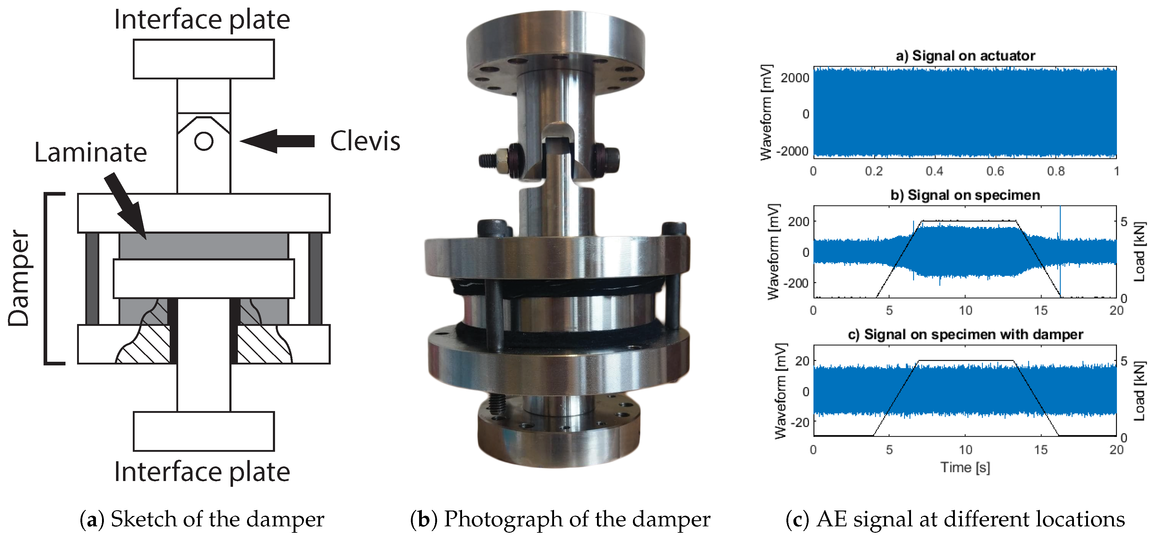
2.2.1. Testing Machine and the Noise Reducing Damper

Servo-hydraulic machines, which are most commonly used in fatigue experiments, are known to produce background vibrations on the actuator and a test piece, arising primarily from servovalves [77,78]. These vibrations often cause uncontrollable fluctuating and load-dependent noise at the output of the AE sensor attached to the test specimen, giving rise to false signals, both continuous and transient, which fall in the frequency and amplitude range comparable to damage-related acoustic emissions, thus making it challenging to remove them in the post-mortem analysis.
To reduce the noise-related artefacts in AE data, several methods have been probed in the research community. These include: (i) passive mechanical dampers installed between the frame, actuator, and the test specimen [77]; (ii) guard sensors and sensor arrays locating the AE signals from the region of interest (e.g., close to the crack tip) [79,80,81,82,83]; (iii) load gating and partitioning the signals with respect to the load (e.g., acquiring the signals which appear only close to the peak load) [84,85]; (iv) setting the high amplitude discrimination threshold [86,87]; and (v) post-processing filtering methods including criterion-based feature selection [88], information entropy-based approach [78], and a variety of hierarchical clustering procedures in an attempt to identify outliers according to distributions of specific features [89].
As will be seen shortly, passive damping is universally efficient and is undeniably recommended for any experimental setup based on servohydraulic or electrodynamic frames. In fact, as has been correctly pointed out by Sauerbrunn et al. [78], neither of the other measures taken individually or in any combination can be considered 100% reliable and universal. We share this opinion, supported by our extensive laboratory experience. Even a very appealing technique of locating AE sources within ROI according to signal arrival times between two or more sensors suffers from substantial drawbacks. To be more specific, it cannot be used for small samples, it fails to work with continuous signals, which are common due to plastic deformation of ductile materials, and, besides, the acquisition system is often overloaded and ceased to operate under cyclic loading due to intensive pulse flow from the area outside ROI. The noise signals and damage-related signals can hardly be distinguished by their frequency spectra, thus making frequency-based filtering ineffective. Needless to say that setting the high amplitude threshold does not help much to solve the machine noise problem as a lot of valuable low-amplitude acoustic information is missed in this way.
Therefore, the present experimental setup is based on the 10 kN electrodynamic Instron E10000 Electropulse universal testing machine. Compared to servo-hydraulic testing frames, a family of modern electrodynamic machines are considerably more silent. Nonetheless, the examination of several electrodynamic machines has shown that they are not completely noise-proof in the dynamic regime and a damper-clevis assembly shown in Figure 2 was installed between the actuator and the specimen grip to reduce the machine noise captured by AE. The clevis joints have a small contact area which helps to reduce the noise. A mechanical damper, inspired by Harris and Dunegan’s early work [77], was made as a laminated structure consisting of numerous aluminium and felt interfaces. The sketch and the photograph of the damper are shown in Figure 2. The signal on the actuator, the signal on specimen without the damper, and the signal on the specimen with the damper installed during cyclic loading of a non-deformable “dummy” specimen are compared in the same figure. One can see that the noise measured on the specimen with the damper was equivalent to the electric background noise at the sensor output.

2.2.2. Fatigue Crack Growth Setup

In this setup, the cameras can run at the same frame rates and similar magnifications, if spatial and temporal synchronisation is of particular concern, or they can run with notably different settings otherwise. For the sake of adaptability to a variety of possible testing conditions, the AE system had its own load-controlled triggering system with a digital oscilloscope to record the load data since the built-in parametric channels in the PCI-2 board operate upon hit-based triggering and are not suitable for continuous recording of external signals. The need for the independent AE trigger is obvious, for a long-term fatigue test, it is virtually impossible to perform the continuous acquisition at 2–5 MSamples/s rate. Therefore, the trigger is programmed to open the AE continuous recording during several consecutive loading cycles. Then, the acquisition stops, and resumes again after the pre-set number of cycles. In this way, the AE system can run independently or synchronously with the cameras.

2.2.3. Tension/Compression Testing Setup

Since the tensile test does not last too long and can be recorded continuously, the main difference between the tensile and FCG setups is in the simplified triggering. A camera with the higher 2448 × 2050 pixel resolution and 15 fps frame rate (Allied Vision Prosilica GC2450 with Tamron 272EN II lens) was used for DIC, if the rapid shooting was not demanded in particular experiments.

2.3. Sample Preparation and Testing Conditions

The material used for the illustration of the capacity of the combination of all chosen in situ techniques with a developed setup was the commercial Inconel-625 alloy with the nominal composition NiCr21Mo8.3Nb3.5 (in wt.%) manufactured by Böhler Edelstahl GmbH & Co KG (Vienna, Austria). The material was annealed at 930 °C for 75 min and quenched in water, resulting in a reasonably uniform microstructure with ≈10 μm grain size. The tensile specimen had a dog-bone geometry with a gauge length of 12 mm, 3 mm width, and 2 mm thickness. The compact tension specimens were made according to the ASTM E647-15e1 standard [90], with 50 mm width W and 4 mm thickness. All specimens were shaped by electric discharge machining.
To facilitate infrared measurements, and improve the signal-to-noise ratio through the increase in the emissivity coefficient of the test object, the dog-bone tensile specimens were coated with a black matt paint (with the emissivity of 0.95) that does not peel off at large strains. The surface facing the DIC camera was additionally covered with white dots sprayed to create a speckle pattern.
The compact tension (CT) specimen for FCG tests were ground down to FEPA #2000 grade. The surface observed by the IRT method was covered with the same black paint, and the RVI side was further treated depending on the purpose of the test. For deformation microstructure observations, the specimens were polished to 1 μm, and optionally etched. For the DIC analysis, the surface was grounded with FEPA #4000 paper in one direction, and random scratches were made with grade #2000 and #4000 papers. If the spatial alignment between the cameras was required, reference lines were made on the surface of the specimen.
Tensile tests were performed under velocity-controlled, nominally constant strain rate of 1 × 10⁻² s−1. FCG tests were performed using the pre-cracked CT specimen cyclically loaded under the load-control mode with the maximum and minimum loads of 7000 N and 1400 N , respectively (the fatigue ratio R = 0.2).

2.4. Data Processing

2.4.1. Tensile Data Processing

The flowchart of data processing involved in the routine tensile test is shown in Figure 3, where data acquired from all four sensors are colour-marked, and the interactions between different data sub-sets and different processing steps are shown by arrows. Sampled load data were interpolated to be aligned precisely with optical images in time. We have chosen the open-source DIC software Ncorr [91] (http://www.ncorr.com (accessed on 24 June 2021)), which allows for creating and building-in the user-made scripts to facilitate the automation of the data analysis process without compromising the quality of the obtained displacements and strain fields [92]. Numerous studies have demonstrated that with the appropriate settings, DIC can capture the strain on the surface of tested with the accuracy comparable to that of high precision extensometers or strain gauges attached to the same specimen [93,94,95]. Specifically, the Ncorr efficiency benefits from the state-of-the art inverse-compositional Gauss–Newton (IC-GN) optimisation algorithm proposed by Pan et al. [96] for fast, robust and accurate full-field displacement tracking with sub-pixel resolution. Leaving the correlation algorithm unchanged, the cross-system data handling and integration software was developed in the present work in MATLAB [97].

Digital Image Correlation

The first step in the processing of images captured by the visible light camera was the DIC analysis. The reference image corresponded to the undeformed specimen. The subset radius was selected between 20 and 25 pixels, and, since the subset spacing reduces the data size, it was chosen to roughly match the size of the images from IRT. For the high strain analysis, the reference image was updated once the correlation became poor. In a later step, the displacements were formatted to be expressed with respect to the initial reference image. With the automatic seed propagation, a seed which is the initial location used for correlation, seeds are updated too. More information can be found in the Ncorr manual [98].
Once the point-wise displacements were calculated, further processing was divided into two distinct parts. In the first part, a virtual extensometer was applied to measure the global engineering and true strain concurrently with the corresponding engineering and true stress calculated using the load signal and the dimensions of the specimen cross-section. In the second part, local deformations and deformation rates were calculated. Ncorr provides displacement fields in the reference and deformed configurations, from which the deformation gradient can be calculated using Equation (1). The property of primary interests, besides the stress and strain, is the mechanical power, which requires the rate of deformation tensor D . This tensor is based on the velocity gradient given in the deformed configuration L , as described by Equation (2), so to express it in the reference configuration, the relation between the deformation gradient in reference configuration and velocity gradient in deformed configuration in Equation (4) was used.
After this step, the displacements, deformation, and deformation rate are known. Calculation of engineering stresses is performed from the load signal and samples geometry. To quantify the overall true stress σ T , the scalar engineering strain ϵ obtained from the virtual extensometer is used, and σ T calculated conventionally as
σ T = P A 0 ( 1 + ϵ )
where P denotes the applied load, A 0 is the initial cross-section. The last expression gives an average value for the region covered by the virtual extensometer in the loading direction. The σ T value provides a good representation of the flow stress as long as the deformation is homogeneous. As soon as the neck sets in, the 1D extensometer data are not accurate any more. An alternative way of estimating the stress tensor is to use the measured local strains in Equation (14) averaged over the cross-section of interest. As long as the deformation is uniform, the results are the same as those estimated from the extensometer. However, measuring local strains yields significantly better stress estimates when strain localisation occurs. Other than longitudinal components in the stress tensor can be estimated from flow rules [99] or from other correction schemes reviewed by Tu et al. [100], if necessary. Once the stress and the deformation rate are known, the mechanical power can be calculated by Equation (5).

Infrared Thermography

Calculations based on infrared thermography data are dependent on the temperature development over both time and space. Since large deformations can be encountered in a tensile test, it might be challenging to track a point on the specimen surface precisely. The sufficiently accurate tracking, however, can be achieved with DIC. To be able to use DIC to track IRT data, the transformation matrix was found between the DIC and IRT images obtained from specific cameras. The transformation matrix maps coordinates from one image to the other. Assuming the deformation pattern is equal on the both opposite surfaces, the displacement field can be transformed to fit IRT data and vice versa. To find the transformation matrix, calibration points, which simply refer to specific chosen locations in an IRT image and a corresponding DIC image, are needed. If there are 3 points, the software finds an affine transformation, and if there are more, the transformation type is projective. The transformation was found using the Matlab embedded function [101]. This procedure and the result are illustrated in Figure 4, where the rightmost image shows a superposition of two images based on the difference between them.
Once the transformation matrix is found, the ROI can be mapped from the DIC optical domain to the IRT temperature domain.
The challenge, which the practitioners usually face with the heat Equation (10), is related to the second-order spatial derivatives. The temperature field measured by the camera is affected by the quality/ or roughness of the surface [102], the texture of the paint, the emissivity of the paint (which is lower than unity, inhomogeneous, and can possibly change during the test, particularly at large strains when the deformed surface gets rough), sensors, internal noise, etc. The inevitable fluctuations in the temperature distribution make the estimation of the second-order spatial derivative a formidable task. The grey-body emissivity correction method using Equation (7) can be employed to reduce the impact of reflections from surroundings. The method is easy to implement as the emissivity is considered to be constant in the narrow spectral band (3–5 μm due to the lens used). Two main assumptions, however, stand behind this method: (i) the grey-body approximation is valid, and (ii) the reflected radiance is represented by the Planck’s function. If the emissivity change appreciably during the test, it must also be accounted for. The error of a black body assumption can be calculated using Equation (6). When the emissivity is high, and the temperature of the specimen is close to the temperature of the reflected surroundings, and the error will be negligible.
Once the temperature field is corrected, noise filtering or noise cancelling procedures are required, although they can introduce some artefacts specific for the filters used. To overcome this problem, the local regression procedure was implemented in the present work. A small circular region close to the point of interest is selected, and a second-order polynomial surface is fitted to it. As long as the heat dissipation is uniform across the chosen region, the temperature within it can be represented very accurately by that polynomial function. However, if the heat dissipation is not uniform, the regression approach causes a smoothing effect: the higher the smoothing factor, the sharper the transitions in the source function. In the tensile test, the heat dissipation is relatively homogeneous as long as plastic deformation is uniform and no local plastic instabilities, such as necking, Lüders bands, or Portevin-Le Chatelier bands show up. In general, the larger the regression radius, the less noise. However, the notice is in place that the regression radius should be small enough to cover the area of the approximately uniform heat dissipation, i.e., the appropriate regression radius depends on the feature size observed in the test. The procedure is illustrated in Figure 5.
The procedure repeats itself for the entire ROI in each image automatically once the operator confirms the satisfactory results of data regression. The results from local regression obtained from IRT data were transformed to fit the DIC data to track the temperature evolution and its Laplacian transform entering Equation (10). The power density of the heat sources is calculated according to Equation (10), and, since the temperature evolution following changes in the heat source was tracked for a given control volume, the power density was integrated over time to find the total energy dissipated at each point of the surface over time. The integration over the volume yields the total power or energy dissipated in the region of interest.
The thermoelastic effect is most significant in the elastic region, and it has only a small effect on the source function in the plastic region. Nevertheless, the source function was corrected for it to give the mechanical power dissipated as heat p D . Once the mechanical work expended for deformation, and the energy dissipated as heat have been simultaneously measured, the first law of thermodynamics can be used to calculate the stored energy [103,104,105,106] (see also a comprehensive review by Bever et al. [107] and references therein). This quantity is of particular interest not only because it relates to the microstructure and deformation mechanisms, but also because it serves as a physically-sound measure of deformation-induced damage. The IRT technique provides a direct estimate of this quantity that is not accessible by in situ measurements otherwise.
As a final note to this session, one can notice that the procedures for joint processing of visual and thermal images could be greatly simplified if thermal and visual cameras were be equipped with lens sets having the same viewing angle and magnification. However, the use of infrared and optical measurements can have different objectives. For the sake of versatility, it is important to keep the possibility to perform the test using different optics on both systems, thus referring to not necessarily exactly the same but overlapping ROI.

Acoustic Emission

The ultimate goal of AE signal processing is to recover properties of the emitting stress relaxation process (or, possibly, multiple processes operating either simultaneously or in a sequence) from the observed data. This pseudo real-time information helps to gain better understanding of underlying accommodative mechanisms active under load. To reduce subjectivity in the interpretation of AE results, the analysis should be non-supervised and data driven. To this end, the processing of the continuously recorded data was performed based on the procedures described in [49]. The continuously streamed acoustic emission data are sectioned into consecutive equal segments of 1024–4096 readings, depending on the temporal scale of the observed transients. After conversion to the frequency domain by the fast fourier transform (FFT), the power spectral density (PSD) function G ( f ) was estimated using the Welch’s method. The AE power P A E of each segment was then calculated as
P A E = f m i n f m a x G ( f ) d f
where f m i n is the high-pass filter cut-off frequency, and f m a x is the Nyquist frequency. The corresponding median frequency, f m was calculated based on the definition through the implicit equation
f m i n f m G ( f ) d f = f m f m a x G ( f ) d f
In order to separate the signals originating from distinct sources (including distinguishing between damage-relates sources and possible outliers and false alarms caused by extrinsic mechanical sources and electrical interferences) the cluster analysis can be performed using the non-supervised data driven adaptive sequential k-means (ASK) algorithm (for mathematical details details of this classifier, readers are encouraged to review the original publication [49]; several successful examples of the application of the ASK algorithm can be found in [35,108,109,110]). The procedure uses a normalised PSD G ( f ) P A E of each data segment as an input for pairwise comparison. It should be noted that due to strong resonance frequencies, which are pronounced even in the broadband commercial sensors, the shape of the PSD is strongly affected by the frequency response of the sensor itself. Therefore, to distinguish between the AE sources based on the evolution of their Fourier or wavelet spectra, it is desirable to use a sensor with the response as flat as possible. Although the AE signal processing software used here does have the intrinsic capacity to perform a versatile cluster analysis after compensation for the background noise, and for the features of the sensor response, we shall not exemplify it in the present work, and the more detailed AE analysis will be reported elsewhere.
The AE signal was synchronised with the video measurements with respect to the moment of failure, which produced a distinct signal with rapid overshooting, and which is easily and precisely identifiable in the AE data. The maximum synchronisation error, in this way, is equal to half of the time elapsed between the last image before failure, and the first image after failure.

2.4.2. Fatigue Crack Growth Data Processing
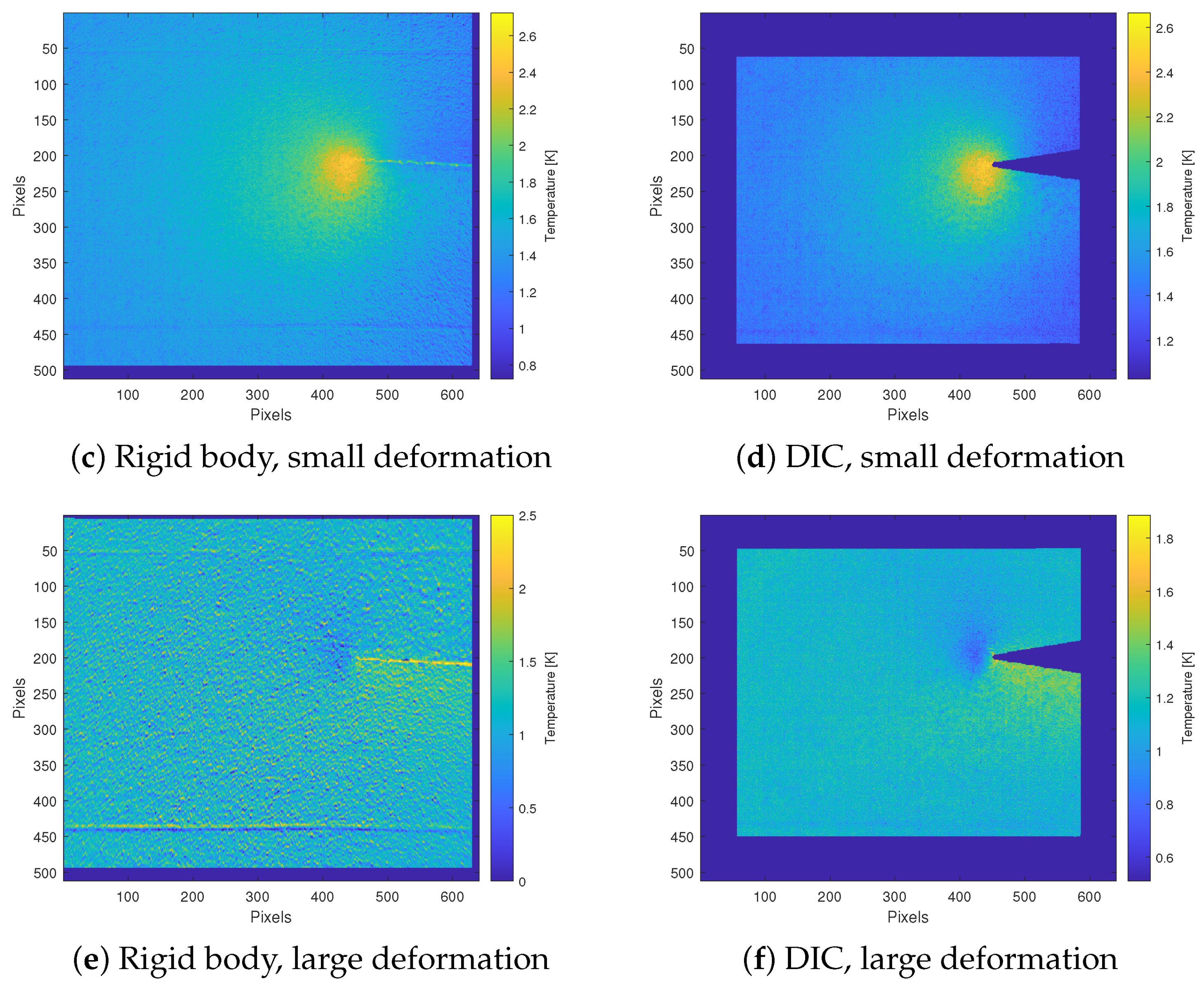
Figure 6 shows the overview of DIC and IRT data processing for a FCG test. Since the AE data processing is essentially the same for both tensile and fatigue crack growth tests, it was excluded from the figure for brevity (see Figure 3 for an overview instead). IRT analysis is divided into three primary steps: (i) locating the crack tip, (ii) finding cameras motion and defining a reference point (feature on the surface) to determine the global position of the crack, and (iii) motion compensation, and data smoothing for spatial and temporal calculations. The DIC method utilises a similar approach for finding global crack properties, e.g., the crack length. Details of processing of FCG DIC and IRT data are provided in Section 2.4.3 and Section 2.4.4, respectively.

Rigid Body Motion

The motion of the camera or the specimen during mechanical testing is inevitable and this needs to be compensated by data processing. The corrective procedure is essentially the same for both DIC and IRT images (with only minor differences between these two), and is, therefore, outlined here. Once two images of interest, which are displaced with respect to each other, are selected, Features from Accelerated Segment Test (FAST) [111] are obtained using Matlab routines [112]. If preferred, ROI from which the features have been extracted can be applied. This is of interest when only a part of the image represents rigid body motion. Further, the features are extracted, and matched, which allows to estimate the geometrical transform between images. Displacements described by this transformation matrix might be caused by the motion of the camera or the specimen. In case of IRT images, they were high-pass filtered and re-scaled before the FAST features were found. Figure 7 shows superposition of two IRT images with two different pseudo colours. Since the camera was moved horizontally between the two to follow the growing crack, there is a displacement between them. ROI was reduced to the left half of the image, to exclude the crack visible on the right-hand side. FAST features are marked with the red circles on image 1, and the corresponding green crosses on image 2. The yellow line between the matched points shows the displacement between them, indicating that the motion between the images was dominated by the translation along the horizontal axis.

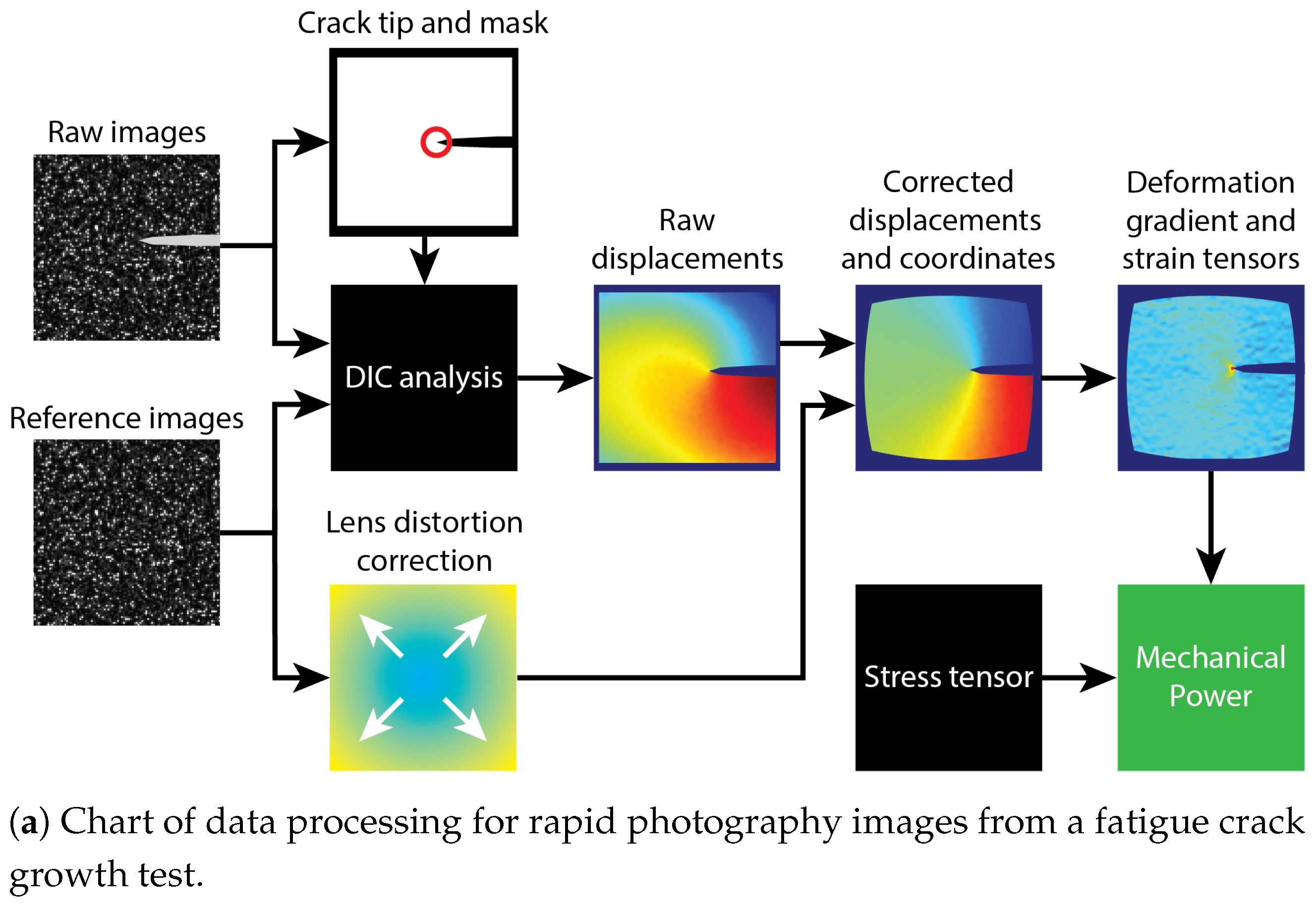
2.4.3. Rapid Video Imaging and Digital Image Correlation

Optical imaging produces a sequence of images, which was used for the DIC analysis. The majority of modifications in the Ncorr codes were made to automate and accelerate the process without affecting the DIC algorithm itself. Each recording was processed individually. The processing was divided into two parts. We first analysed the entire sequence of images with respect to the “cyclic” reference image taken close to the mean load immediately after the test was paused. In a second part of the analysis, we compared two reference images: the “cyclic” reference image corresponding to the finally deformed state and the one of the undamaged sample. The second step allowed us to find the total strains with respect to the undeformed specimen. However, when plastic deformations are large, the surface becomes so severely deformed that the correlation between the undeformed and finally deformed specimens is not reliable any more or it can disappear completely. Nonetheless, the analysis of the image sequence with respect to the cyclic load can still deliver the rate of the deformation tensor as a function of the number of cycles.

Region of Interest and Mask

To ensure a high quality of strain data in the vicinity of the crack tip, the crack representing discontinuity in strain data must be covered by a virtual mask. If the mask is too wide, valuable data in close proximity to the crack path might become lost, whereas if it does not cover the crack sufficiently, incorrect strain values can be obtained. The precise determination of the crack tip position is, therefore, of crucial importance. There have been many methods proposed in the literature to find the crack tip position (see [15,57,113,114] and references therein). The approach we utilised in the present work is based on the simple observation that the crack was dark, and it was well visible throughout the test. A convolution algorithm was developed to find this dark region, and the end of it was defined as the crack tip. Additionally, the images corresponding to the maximum and minimum load were used to find the motion range within a given recording to make sure the mask was created sufficiently within the borders of the field of view (FOV). An example of the DIC mask created by this algorithm is shown in Figure 8.

DIC Analysis

Once the images are chosen for the analysis and the mask is applied, the seed points are selected. The algorithm for that was based on Speeded Up Robust Features (SURF) [115], as the features identified in this way are good candidates for distinct points. A similar approach was used by Wang et al. [116]. SURF points were found in the reference image, and they were classified according to their strength. The number of points corresponding to the number of processor threads was selected. To make sure that they were roughly equally spaced, the chosen points were placed as far away from ROI borders, and from each other as possible. Hence, the region for the analysis was approximately evenly distributed between the CPU threads for efficient computation. Once all of these steps were automatised, the DIC analysis could run automatically.

Correction for Lens Distortion

Like the majority of microscopic lenses, the lens used for FCG tests distorts the image. The Ncorr DIC algorithm has a rather simple way for accounting for the error in displacements caused by lens distortions, provided the lens distortions are known. To quantify and eliminate the distortions, the method proposed by Pan et al. [117] was employed. The linear least-squares algorithm estimates the distortion coefficient from the distorted displacements obtained from the rigid body, in-plane translation DIC analysis. Ncorr utilises this coefficient to correct the distorted displacement fields. Corrected displacements are, however, still in distorted coordinates. This affects the strain calculations, as the Ncorr algorithm assumes an equal and constant spacing between points, which is not the case with non-negligible lens distortions. To express the displacements in undistorted coordinates, first the valid undistorted coordinates within the analysed region were found. The mask containing the valid pixel locations was undistorted, creating a new mask consisting of undistorted coordinates. To find the displacements in the undistorted coordinates, the equivalent distorted coordinates were calculated with the distortion model. Eventually, the displacement data could be interpolated at these locations, resulting in displacements in the equivalent undistorted coordinates. Results for raw and corrected displacements are exemplified and compared in Figure 9: owing to these implemented measures, the improvement of displacement measurements after lens distortion correction is remarkable, which, in turn, results in the enhanced accuracy of strain field estimates.

Deformation Gradient and Strain Tensors

Once the coordinates and displacements have been corrected, the strains can be seamlessly calculated using the deformation gradients calculated by Ncorr. As a result, the displacement vector u is obtained in the reference and deformed configurations, X and x , respectively, as well as the derivatives of the displacement vector with respect to coordinates in both configurations.
The global displacement field between the undeformed and cyclically deformed material is denoted as u c u . Images obtained during cyclic test were processed one by one with respect to the “cyclic reference” image, which was acquired immediately after the cyclic images. The data for this sequential cyclic analysis will be denoted by the subscript index c ( u c , x c , X c ), and data from the analysis with undeformed body will have the subscript index u ( u u , x u , X u ). Since u = x X , and X c = x u , we can express u u as
u u = X c X u
The goal is to find the deformation gradient as if the cyclic analysis would be performed with respect to the undeformed state, u c u X u . After differentiating Equation (17) with respect to X c , and rearranging it, we obtain
X c X u = I u u X c 1
Since u c u X c = u c X c + u u X c , and both terms on the right hand side are known from the DIC analysis, it can be combined with Equation (18). Hence, the deformation gradient defined with respect to the undeformed configuration ( F ) can be expressed as
F = I + u c u X u = I + u c u X c · I u u X c 1
Once the gradients with respect to both the cyclic reference image and the undeformed material are known, the strain tensors of interest can be calculated. The polar decomposition theorem can be used to decompose the F tensor into a product of two second-order tensors and, thus, to separate the rotation matrix R and the right stretch tensor U as
F = R · U
Since R T · R = I (the superscript T denotes the transpose), the rigid body rotations are eliminated, and the right stretch tensor can be determined from the relation
U 2 = U T · U = F T · F = C
which also defines the right Cauchy–Green deformation tensor C . Since F is known, the deformation rate tensor D can be calculated straightforwardly by combining Equations (2) and (4).

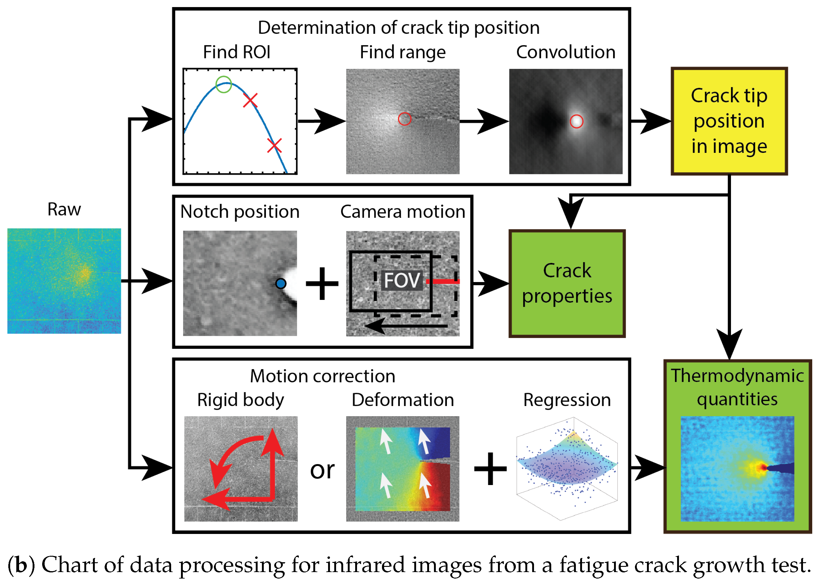
2.4.4. Fatigue Crack Growth Data from Infrared Thermography

Finding the Crack Tip Position

To determine the crack tip position, we combine the thermoelastic effect and the heat dissipation measurements. The idea is to take the data recorded just after peak load, where the load decreases while the crack closure effect is negligible. At this stage, both the thermoelastic effect and the heat dissipation (if any) contribute to the temperature rise, with the maximum reached at the crack tip. The region behind the crack tip should experience a lower temperature change, as the closure effects are not active, and the stresses are comparatively low. The images taken at the upper and lower limit (marked with red in Figure 10) were stabilised with respect to the cyclic reference image—the image taken immediately after the test interruption at the mean load. The procedure was essentially the same as that described in Section 2.4.2 with one correction: the transformation matrix was used to transform the images with an affine transformation to the reference image to find the temperature change between the images. By applying convolution with a specific kernel, which added the data covered by a 90 degree angle in front of a point of interest, and subtracted an equivalent region behind it, the sharp changes are maximised, and the crack tip can be easily located at the brightest point of the convoluted image as illustrated in Figure 11, comparing the temperature change map and the corresponding result of the convolution operation. The image can suffer from noise caused by the uncoated metallic surfaces at the crack faces. Therefore, the local extreme temperatures in the area outside the high temperature region surrounding the crack tip were replaced with the mean temperature for a given image.

Motion Compensation and IRT/DIC Algorithm

To measure and minimise the effect caused by the camera motion between recordings sessions, the cyclic reference image in each session was used. The procedure explained in detail in Section 2.4.2 was used to find the displacement between the images induced by the camera motion. ROI was selected to be approximately equal to half of the image without the crack. Since there is no crack in ROI, all deformations are relatively small, and the rigid body assumption holds. Figure 7 represents an example of finding how far the IRT camera has moved between two successive recordings. The transformation matrices can be combined to express the position of each reference image with respect to the first one (in any coordinate system chosen). Marking the notch position in an image, and finding its transformation matrix with respect to the first reference image, allows determining the crack position with respect to the notch. It is also possible to create a specific user-preferred coordinate system.
Tracking data points in a record can be performed in two ways. The first way is to use a geometric transform (Section 2.4.2) based on the rigid body motion assumption, which is justified for small deformations. Alternatively, one can perform the correlative analysis of images based on IRT data, which can be used to estimate local displacements in many practical situations, where the optical imaging is difficult. The quality of these estimates depends heavily on the quality of IRT images. A very elegant approach has been proposed by Maynadier et al. [118] who applied the DIC technique to the images captured with an infrared camera in order to obtain perfectly synchronised kinematic and thermal full-field maps solely from the calibrated infrared measurements. Inspired by this work, we propose a simplified algorithm giving rise to similar results, although the quantitative comparison of the accuracy achieved by these two methods has not been performed yet.
In our approach, the DIC/IRT pattern for correlation is based on the texture of the high emissivity paint. The benefit of this approach is that since the whole ROI is painted, the thermal measurements are not affected by low emissivity speckle pattern needed for conventional DIC, and the correlative analysis can be completed using only IRT images with little effort. Some image preparation is, however, required since the temperature data are obtained from a camera in a single precision floating point format, whereas the DIC software works with the 8-bit unsigned integer format. To convert the data to the format digestible by the DIC algorithm, IRT images are filtered by a conventional Gaussian filter with the degree of smoothing adjusted for the feature size. From experience, we set the standard deviation of the Gaussian kernel function at 6 for the cases considered here. The smoothed images were subtracted from the original images, unveiling the paint texture. Any values deviating from means for more than five standard deviations (measured for the distribution of intensity over the entire image) after filtering, were replaced by the five standard deviations limit, to reduce the influence of noise on rescaling of images when converting them to 8 bit format. To proceed with the DIC analysis, a virtual mask covering the crack was applied using the crack location data determined in Section 2.4.4.
The IRT-based DIC processing yields the displacement values evolving during cyclic loading. By subtracting the initial image corresponding to the undeformed state from the sequence of images representing the cyclically deformed state, one obtains the local temperature increments in the reference and deformed configurations. The background image subtraction removed most of the texture visible in the raw images. Figure 12 shows a comparison of the raw image (a), reference image of undeformed sample (b) and the results of subtraction based on rigid body motion correction (c,e), and DIC-based motion correction (d,f). When deformations are small, the rigid body correction scheme might be sufficient (cf. (c,d)), while when the deformations become larger, the rigid body correction gives rise to the noisy texture pattern in the temperature field (e), whereas the IRT/DIC-based correction (f) still shows good results.

Local Regression

The approach for local regression is similar to the one used for the tensile tests. A reference image taken before the beginning of the test was subtracted from all images acquired during cyclic testing, and the ROI from the IRT/DIC analysis for the motion compensation was used. At each pixel position within the global ROI, a smaller circular region was selected with a radius of 10.5 pixels, and the data within that region were used to fit by a second-order polynomial function. The second-order spatial derivative of the temperature, as well as other spatial properties, can be extracted directly from the fitting function afterwards.

2.4.5. Spatial and Temporal Calculations

Aiming at obtaining the source function q ˙ from the heat Equation (10), one needs to proceed with numerical derivatives of the temperature with respect to time and coordinates. The value of the temperature rate T t can be calculated based on the motion correction. The input images can be either raw images with or without background subtraction, or the temperature field extracted from the regression analysis. The temperature distribution obtained after regression is smoother, as the regression exerts the effect similar to low-pass filtering. In the particular tests exemplified in the present work, the regression data were used to calculate both the temporal and spatial derivatives of the first and second order, respectively. Ideally, when no heat dissipation occurs, and the temperature field reaches equilibrium, the second derivative should be zero. It is, therefore, possible and reasonable to subtract the Laplacian term obtained for the reference image taken after the test has been paused, i.e., when no heat dissipation occurred, from all images in the recording session. This step allows to remove remaining occasional systematic noise, if it exists and is seen in the Laplacian term.

3. Illustration of the Proposed Approach: Results of Case Studies

The proposed in situ characterisation methodology has been probed on tensile and FCG testing of the Inconel-625 alloy, representing a family of solid solution hardening nickel-based super-alloys having an excellent combination of high strength, ductility, corrosion, and heat resistance. Due to its outstanding properties profile, this alloy has found widespread applications in aeronautic, aerospace, chemical, and petrochemical industries, marine, and nuclear power engineering. For the purpose of the present work, this material was chosen due to a combination of its high density and relatively low electrical and thermal conductivity, favourable for IRT measurements. The microstructure of the Inconel-625 alloy depends on the applied heat treatment [119], and consists typically of the austenitic fcc  γ -phase matrix containing several secondary strengthening phases including carbides, γ , and γ precipitates. The main findings are summarised as follows.

3.1. Tensile Test

Figure 13 shows the true stress-strain curve and the expended mechanical power density p M (estimated by using DIC mapping and averaged over the entire specimen gauge part) and its variance as a function of strain. The strain hardening rate θ ( ε T ) = d σ T d ε T was calculated and its fragment is shown in the figure to highlight the crossover with the σ T ( ε T ) indicating the onset of necking according to the Considère criterion (cf. [120,121,122] for other forms of instability criteria based on the evolution of the total dislocation density)
d σ T d ε T = σ T
The alloy demonstrates an excellent hardenability resulting in the true strength exceeding 1.3 GPa and uniform strain up to 0.35 before the Considère condition is met.
One can notice that the mechanical power exhibits interesting behaviour, the details of which unveil several deformation stages, as will be discussed in what follows. The distribution of locally measured p M values is of its own interest, and is shown in Figure 14 representing three typical situations marked in Figure 13: (a,b) the onset of plastic yielding when the Lüders band forms at the upper edge of the gauge part of the specimen; (c,d) the uniform deformation stage; (e,f) the developed necking stage. During uniform deformation, the p M distribution has a symmetric Gaussian shape, which is reasonably expected for this stage. Not only does the distribution of p M become significantly skewed towards the left hand-side of the histograms (i.e., the most probable values lie in the low power domain, indicating that most parts of the specimen do not deform plastically) when the strain localisation occurs, but also its variance can serve as a measure of strain localisation. Indeed, Figure 13 illustrates it explicitly—the variance of the p M distribution increases dramatically when necking sets in under plane stress domination at the necking strain ε N = 0.35 (it should be, however, noticed, that the accelerated increase in the p M variance becomes appreciable even before the macroscopic loss of stability commences according to the mechanistic criterion from Equation (22). Outside of the neck region, the material, however, slightly unloads since the global reaction force decreases in response to the shrinking cross-sectional area within the neck [123], thus resulting in some negative values in the mechanical power distribution shown in Figure 14e.
Figure 15 compiles the results from all of the methods in a single plot: (i) the average expended mechanical power density is plotted in parallel with the dissipated and stored power, and all curves are synchronised with the stress-strain data. The strain hardening rate is also plotted for comparison.
The typical evolution of the AE signal in the Inconel-625 alloy is illustrated in terms of the dissipated AE power P A E and the median frequency f m of the PSD function synchronised with the tension loading curves and strain hardening rate. Analysis of Figure 15 reveals that, typically for ductile materials, AE commences already at the relatively low applied stress and peak when the Lüders band nucleates and propagates. Then, the AE level decreases continually until fracture, but never vanishes. Overall, AE exhibits the behaviour typical of metals and alloys with dislocation-mediated plasticity [38,124]. While the power (or energy) reduces with strain in response to strain hardening and the concomitant shortening of the dislocation mean free path, the median frequency f m of the PSD increases steadily for the same reason in parallel with the flow stress. This trend in the f m behaviour is confirmed in Figure 15—as long as plastic deformation is uniform, the average f m value increases steadily. However, when the deformation begins to localise in a neck, the local strain rate increases drastically relative to that outside the neck. In response to this, f m rises steeply, which is in qualitative agreement with the linear strain rate dependence of the AE median frequency proposed in [124].
The behaviour of the strain hardening rate indicates that uniform plastic deformation proceeds through different stages (the yield point followed by the Lüders band propagation, and stages II and III can be discerned from the θ ( ε T ) behaviour). The same stages can be seen, in principle, in the evolution of the average total mechanical power p M . The dissipated p D and stored p S powers exhibit opposite trends in the necking region: while the former shows a sharp increase, the latter changes its trend from ascending to descending. The smooth gradual increase in p D and p S with strain is observed in parallel with the progressive rise in the AE median frequency changing with the evolution of the dislocation microstructure. The overall strain hardening behaviour is nicely reflected by the AE power, which behaves in general agreement with the predictions of the phenomenological model of AE caused by dislocation-based strain hardening proposed in [125]. Specifically, the increased AE activity is noteworthy at approximately 0.07 strain, where the transition between Stages II and III can be seen in the behaviour of θ ( ε T ) and p M ( ε T ) . The in-depth discussion of the observed trends requires a bridge to be built between the thermodynamics of plastic deformation and the underlying microstructural evolution, which is beyond the scope of the present paper and will be discussed elsewhere. Nonetheless, importantly for the purpose of the present work, the proposed methodology, based on a comprehensive in situ monitoring strategy, follows the evolution of the microstructure with strain hardening, and provides the grounds for the progress in the thermodynamic analysis of plastic deformation.

3.2. Fatigue Crack Growth Test

In the fracture mechanics approach to the stable fatigue crack propagation, in the vast majority of structural materials, the crack length a increases under cyclic load according to the empiric Paris–Erdogan equation
d a d N = C Δ K m
where d a d N represents the crack growth rate (the crack length increment per cycle), and C and m are experimentally determined material properties known as Paris coefficient and Paris exponent, respectively (both dependent also on the environment, temperature and loading conditions). Figure 16 shows the Paris plots for the crack growth rate d a d N vs. the stress intensity factor range Δ K , which are obtained independently from the IRT (a) or RVI (b) data used to find the crack tip position and estimate the crack length. The vertical lines indicate the validity of the linear elastic fracture mechanics (LEFM) and the Δ K concept according to the ASTM standard [90], which is verified by the criterion:
( W a ) 4 π K m a x σ y s 2
where W is the effective width of the specimen, a is crack length, K m a x is the highest stress intensity factor occurring within a cycle, and σ y s is the materials yield stress. The stress intensity factor needs to be calculated within the small scale yielding (SSY) approximation of an elastic-plastic body with a Mode I crack in plane strain. In Figure 17, the results from both techniques are compared. Not only an excellent agreement between both methods is seen, but also the scatter of experimental data for d a d N for each technique is reasonably small. Both methods yield practically the same Paris parameters C and m of 3.12 ± 0.03 . Additionally, for both methods the slight deviation from the LEFM prediction according to the Paris’ law becomes visible precisely at Δ K expected from the SSY criterion of 62 M Pa m corresponding to the crack length a of 24.8   m m .
The reversible thermoelastic effect and the irreversible heat dissipation due to plastic deformation in the cyclic plastic zone are the two main contributors to the heat source function q ˙ in Equation (10). Since the thermoelastic effect assumes the linearity between the stress and temperature increment, one can make use of the cyclic loading to eliminate this effect from the analysis by performing the integration of the q ˙ over each loading cycle. An example of the heat dissipation behaviour per cycle is illustrated in Figure 18, where the heat power density q ˙ at the crack tip is plotted versus the applied load. An example of the map of the energy dissipated during one cycle w D is shown in Figure 18c, highlighting the cyclic plastic zone ahead of the crack tip.
The plot compiling the main findings from all three in situ methods is represented in Figure 19, where the average (per cycle) AE energy and median frequency are plotted together with the dissipated heat energy at the crack tip as a function of the crack length, which serves as a damage parameter for FCG. The load gating method was used to select the AE signals at the loads exceeding 0.95 of the peak load, and to remove the signals associated with crack closure on unloading. As a note, AE due to crack closure can be produced by several mechanisms such mechanisms as rubbing of the crack faces due to local compressive stresses from plastic deformation, friction between jagged crack edges and rubbing or breaking of wedged oxides [126,127,128,129,130]. AE induced by crack closure is dependent on many factors including materials properties, environment, and test frequency [86,127]. The ductility of the material affects the roughness of the crack faces, and the susceptibility of a material to oxidation in a given environment will affect the presence of oxides in the crack region. Closure emissions are generally unwanted in the AE analysis of FCG [126], unless the crack closure phenomenon itself is of particular interest. Before discussing the AE findings of the present work, a brief excursion to the FCG related mechanisms would be in place. Acoustic emission from fatigue crack-related mechanisms has been studied experimentally for decades, and AE features specific to crack initiation, crack extension, and crack closure have been identified by many researchers on examples of various materials. Several empiric relations and qualitative explanations of the crack growth behaviour in its relation to AE have been developed, and some are described below. Fracture mechanisms associated with the opening of new surfaces and expansion of the plastic zone during crack extension produce elastic waves. The amplitude of the AE signal depends on the dynamics at the source [131,132], and, in general, brittle fracture mechanisms produce higher amplitude signals than ductile ones [129,133,134,135]. Brittle fracture mechanisms include intergranular and cleavage fracture. Ductile fracture mechanisms involve microvoid nucleation and coalescence, tearing, and shearing. Pollock [136] considered the elastic energy conversions of a system during crack growth for characteristic ductile and brittle source events of equal magnitude. The difference in the AE signal amplitudes was explained by partitioning the released energy into three groups: energy of plastic deformation, surface energy or “event” energy associated with AE waves. The plastic deformation term captures the energy expended in creating the plastic zone through the dislocation generation and movement, while the surface energy refers to the disbonding of the single atomic layer to create the new surfaces. It was argued that due to a larger plastic zone and the increased surface energy due to a rougher crack surface, a lesser fraction of the released elastic energy is emitted as AE in the ductile fracture mode compared to brittle fracture of the same magnitude of the energy release at the source. For FCG, Morton et al. [137,138] found a relation between the AE count rate d N A E d N , and ΔK in the form of the power law resembling the Paris–Erdogan FCG Equation (23) (see also [77,139,140], where the first model has been proposed to link the AE count rate with the stress intensity factor):
d N A E d N = C A E Δ K n A E
where C A E is the empiric constant and the exponent n A E is found to be related to the Paris exponent, m, by the relation n A E m + 2 as proposed by Lindley et al. [129]. It was suggested that both the energy released during crack extension, and the deformation and fracture related events within the plastic zone ahead of the crack, contribute to AE during FCG, see Heiple and Carpenter [141,142], finding dislocation mechanisms, twin nucleation, and fracture of inclusions to be potent sources of AE in the plastic zone.
For the material under investigation, the mechanisms related to mechanical twinning and fracture of hard particles can be ruled out due to Inconel’s high stacking fault energy. Therefore, the primary energy dissipation mechanisms are supposed to be attributed to the crack advance and the dislocation activity in the plastic zone. One can note that, in line with many previous observations, the average (per cycle) AE power increases exponentially as the crack advances. Even though the observed behaviour of the AE power P A E presented in Figure 20 as a function of Δ K can be approximated by a straight line in log-log scale, the linear fit is applicable only for the low Δ K domain. It is interesting that the power relation (25) holds reasonably only up to the critical Δ K value corresponding to the LEFM limit, whereas beyond this point, the AE power tends to increase rapidly with the crack advance, which agrees with the development of the excess plasticity ahead of the crack tip. However, the observed behaviour contradicts the predictions by Lindley et al. [129] since the n A E value of 2.2, which is obtained from the least square fit in Figure 20, is far from being equal to m + 2 at relatively small Δ K , as anticipated from the cited work for the AE count rate [129]. Thus, even though there seem to be a reasonable agreement between the AE power and the stress intensity factor range indeed, at least within small scale yielding, there is still no consensus about the n A E index, and there is still a big deal to establish the dependence (if any) of n A E on the microstructure and testing conditions. Figure 19 unveils another interesting correlation between the AE power, the heat dissipation power, and the strain range. The latter quantity assessed by DIC as the difference between maximum and minimum local strain per cycle serves as a measure of the expended mechanical power in the plastic zone. One can notice that the measured strains appeared to be substantially plastic (see the blue curve in Figure 19, which represents the strain range measured by DIC). Therefore, obtaining the expended mechanical power from DIC is not as straightforward as that in the case of uniaxial tension. Nonetheless, the observed correlation is noteworthy and the expended mechanical power can be obtained in a more elaborated approach.
Although the AE power (energy or count rate) has long been recognised to be generally related to the fatigue crack length or the stress intensity factor range, the behaviour of the AE spectral density during fatigue crack propagation has not been explored so far, to the authors best knowledge (that is at sharp contrast to the monotonic tensile testing). In the present work, we illustrate the evolution of the AE PSD function by the behaviour of its median frequency (compare to that in the tensile test, Figure 15). As cycling proceeds and the crack advances, f m shows a general trend to decrease (Figure 19). This apparent trend opposes that in monotonic tension, where the f m value increases with strain hardening, as has been discussed above. According to the statistical interpretation of the median frequency as a property reciprocal to the correlation time in the ensemble of emitting defects proposed by Vinogradov et al. [25] (see also [124]), the increase in the f m value signifies the increase in randomness of AE sources, while the opposite trend (decreasing f m ) heralds the increase in their temporal correlation or spatial scale. This interpretation appears to be in harmony with the observed behaviour of f m , since during FCG the plastic zone expands progressively at the expense of the undeformed material, resulting in longer and longer crack jumps. Thus, AE is emitted not from the most heavily deformed plastic zone, but primarily from its expanding periphery, thus involving greater and greater undeformed volume into the process of cyclic plastic zone growth. What should be noticed in the behaviour of the AE median frequency is that it exhibits a local maximum at the intermediate Δ K values. Presumably, this specific behaviour reflects the AE PSD response to the local strain hardening in the growing plastic zone. This process was not visible in the very small plastic zone at the beginning of the crack growth. As the plastic zone increased the contribution of strain hardening became appreciable in the AE PSD evolution. The gradual shift of f m towards the higher frequency domain was finally overridden by the rapid development of the excess crack tip plasticity beyond the LEFM SSY limit resulting in the rapid expansion of the plastic zone and the reduction in AE PSD.
Concluding this section, a brief discussion regarding uncertainty of the measurements is required. Similarly to many commercially available infrared cameras with cooled quantum sensors, the factory-calibrated TELOPS FAST M350 thermograph used in the present work delivers a radiometric temperature accuracy of 1 K (or ±1% over the entire range), which is not very impressive, yet typical in the class. The energy calculations are, however, based on the spatio-temporal difference in the temperature. The resolution related to the temperature increment is, fortunately, much better, reducing ideally to 20 m K , as has been discussed above. The greatest uncertainty in the estimates of the thermodynamic quantities, such as a stored energy, is known to be associated with the measurements of the temperature rate and the Laplacian of the temperature field. We have not performed the formal differential error analysis of the propagation of uncertainty in our measurements of quantities entering Equations (10) and (13). However, based on the “worst case” analysis, the relative uncertainty in the estimated stored energy does not exceed 15% over the entire range, and this is the most conservative estimate. Furthermore, the calibration procedure applied to the IRT system supports the opinion that 15% can be regarded as the upper boundary in uncertainty, and is likely to be notably smaller. The propagation of error analysis and the details of the calibration procedure, which itself might be of special interest, will be reported elsewhere. In brief, the well-controlled rectangular DC current pulses of 2, 5, 10, 20, and 50 A amplitude and 200 ms duration were passed through the Inconel-625 test specimen (being initially at room temperature), and the corresponding voltage drops and Joule heat dissipation were independently measured. The temperature rise did not exceed 7 K at 20 A, and 55 K at 50 A current. Regardless of the magnitude of the temperature rise, the measured thermal power consistently compared favourably to the measured Joule heat (electric power). This justifies that the obtained estimates of the thermodynamic quantities are reliable that the procedures used to obtain them are adequate.

4. Summary, Conclusions, and Future Scopes

As a final comment, the preliminary results from the case study on the tensile and fatigue behaviour using the fcc Inconel-625 alloy as an example contain a wealth of information regarding underlying deformation and fracture mechanisms. This multifaceted information was enabled due to the integration of several in situ monitoring techniques—infrared thermography, multi-resolution rapid video imaging complemented by the digital image correlation capability, and acoustic emission powered by the spectral analysis and statistical clustering algorithms—into a common framework, addressing multiple hardware and software challenges, which are inevitable in a contemporary advanced experimental design. At variance to the commercially available systems pairing the DIC and IRT techniques (e.g., https://www.infratec.eu/thermography/digital-image-correlation-and-thermographic-measurements/ (accessed on 14 July 2021)), the use of the open-source software architecture offers uncompromised versatility with a balance of efficiency, accuracy, and tunability of the entire system. Not only the proposed system can be adapted to virtually any combination of thermal and visual cameras, and to suit a wide range of load-bearing applications, but also the concurrent use of AE measurements, which are fully synchronised with the two other techniques and the loading device, adds a new dimension to the multiscale research in the field of physics and mechanics of plasticity and fracture.
Admittedly, the presented results show only the tip of the iceberg and leave more questions than answers. Specifically, there is still a great deal of opportunity to improve virtually all metrological aspects and traceability of the results of measurements by the techniques employed. However, we believe that the proposed rigorous methodology documented in significant details in the present communication permits answering many open questions related to damage initiation and propagation in solids under monotonic and cyclic loads. This is the scope of the ongoing research, the results of which will be reported elsewhere. We also believe that the proposed instrumented laboratory experimental platform can serve for future developments of novel practical approaches and means for non-destructive health monitoring of industrial facilities and infrastructure.

Author Contributions

Conceptualisation, A.S. and A.V.; methodology, A.S. and A.O.M.; software, A.S.; validation, A.S.; investigation, A.S., A.O.M. and S.W.W.; writing—original draft preparation, A.S., A.O.M. and S.W.W.; writing—review and editing, A.V., A.S. and A.O.M.; visualisation, A.S.; supervision, A.V. All authors have read and agreed to the published version of the manuscript.

Funding

This work was partially supported by Research Council of Norway, Project No. 294739, Safe Pipelines for Hydrogen Transport (HyLINE).

Institutional Review Board Statement

Not applicable.

Informed Consent Statement

Not applicable.

Data Availability Statement

Data are available from the corresponding author upon reasonable request.

Acknowledgments

The authors gratefully acknowledge to T. Kristensen and SINTEF Industry personnel for their kind help with specimens preparation. Special thanks go to A. Alvaro and F. Berto for encouragement, support, and discussions. We also thank R. Johnsen for providing the material for this study. The authors would like to thank the anonymous reviewers for the insightful comments that helped in improving the manuscript.

Conflicts of Interest

The authors declare no conflict of interest.

Abbreviations

AEAcoustic emission
DICDigital image correlation
FASTFeatures from accelerated segment test
FCGFatigue crack growth
FFTFast Fourier transform
FOVField of view
IBRIn-band radiance
IRTInfrared thermography
LEFMLinear elastic fracture mechanics
MOIMoment of interest
NETDNoise equivalent temperature difference
PSDPower spectral density
ROIRegion of interest

References

  1. Sutton, M.A. Digital Image Correlation for Shape and Deformation Measurements. In Springer Handbook of Experimental Solid Mechanics; Sharpe, W.N., Ed.; Springer: Boston, MA, USA, 2008; pp. 565–600. [Google Scholar] [CrossRef]
  2. Mountain, D.; Webber, J. Stress Pattern Analysis by Thermal Emission (SPATE). Proc. SPIE 1979. [Google Scholar] [CrossRef]
  3. De Finis, R.; Palumbo, D.; Galietti, U. A multianalysis thermography-based approach for fatigue and damage investigations of ASTM A182 F6NM steel at two stress ratios. Fatigue Fract. Eng. Mater. Struct. 2019, 42, 267–283. [Google Scholar] [CrossRef] [Green Version]
  4. Morabito, A.E.; Chrysochoos, A.; Dattoma, V.; Galietti, U. Analysis of heat sources accompanying the fatigue of 2024 T3 aluminium alloys. Int. J. Fatigue 2007, 29, 977–984. [Google Scholar] [CrossRef]
  5. Berthel, B.; Chrysochoos, A.; Wattrisse, B.; Galtier, A. Infrared image processing for the calorimetric analysis of fatigue phenomena. Exp. Mech. 2008, 48, 79–90. [Google Scholar] [CrossRef]
  6. Zhou, W.; Han, K.N.; Qin, R.; Zhang, Y.J. Investigation of mechanical behavior and damage of three-dimensional braided carbon fiber composites. Mater. Res. Express 2019, 6, 085624. [Google Scholar] [CrossRef]
  7. Díaz, F.A.; Patterson, E.A.; Tomlinson, R.A.; Yates, J.R. Measuring Stress Intensity Factors during Fatigue Crack Growth Using Thermoelasticity. Fatigue Fract. Eng. Mater. Struct. 2004, 27, 571–583. [Google Scholar] [CrossRef]
  8. Meneghetti, G.; Ricotta, M.; Pitarresi, G. Infrared thermography-based evaluation of the elastic-plastic J-integral to correlate fatigue crack growth data of a stainless steel. Int. J. Fatigue 2019, 125, 149–160. [Google Scholar] [CrossRef]
  9. La Rosa, G.; Risitano, A. Thermographic Methodology for Rapid Determination of the Fatigue Limit of Materials and Mechanical Components. Int. J. Fatigue 2000, 22, 65–73. [Google Scholar] [CrossRef]
  10. Lipski, A. Rapid Determination of the S-N Curve for Steel by Means of the Thermographic Method. Adv. Mater. Sci. Eng. 2016, 2016, e4134021. [Google Scholar] [CrossRef] [Green Version]
  11. Ancona, F.; De Finis, R.; Demelio, G.P.; Galietti, U.; Palumbo, D. Study of the Plastic Behavior around the Crack Tip by Means of Thermal Methods. Procedia Struct. Integr. 2016, 2, 2113–2122. [Google Scholar] [CrossRef] [Green Version]
  12. Fedorova, A.Y.; Bannikov, M.V.; Bannikov, M.V.; Plekhov, O.A.; Plekhova, E.V. Infrared thermography study of the fatigue crack propagation. Frattura ed Integrità Strutturale 2012, 6, 46–53. [Google Scholar] [CrossRef] [Green Version]
  13. Ju, Y.; Xie, H.; Zhao, X.; Mao, L.; Ren, Z.; Zheng, J.; Chiang, F.P.; Wang, Y.; Gao, F. Visualization method for stress-field evolution during rapid crack propagation using 3D printing and photoelastic testing techniques. Sci. Rep. 2018, 8. [Google Scholar] [CrossRef]
  14. Hertegård, S.; Larsson, H.; Wittenberg, T. High-speed imaging: Applications and development. Logop. Phoniatr. Vocol. 2003, 28, 133–139. [Google Scholar] [CrossRef] [PubMed]
  15. Gao, H.; Zhang, Z.; Jiang, W.; Zhu, K.; Gong, A. Deformation Fields Measurement of Crack Tip under High-Frequency Resonant Loading Using a Novel Hybrid Image Processing Method. Shock Vib. 2018, 2018. [Google Scholar] [CrossRef] [Green Version]
  16. Seleznev, M.; Vinogradov, A. Note: High-speed optical imaging powered by acoustic emission triggering. Rev. Sci. Instrum. 2014, 85, 076103. [Google Scholar] [CrossRef] [PubMed]
  17. Hosdez, J.; Witz, J.F.; Martel, C.; Limodin, N.; Najjar, D.; Charkaluk, E.; Osmond, P.; Szmytka, F. Fatigue crack growth law identification by Digital Image Correlation and electrical potential method for ductile cast iron. Eng. Fract. Mech. 2017, 182, 577–594. [Google Scholar] [CrossRef] [Green Version]
  18. Carroll, J.D.; Abuzaid, W.; Lambros, J.; Sehitoglu, H. High resolution digital image correlation measurements of strain accumulation in fatigue crack growth. Int. J. Fatigue 2013, 57, 140–150. [Google Scholar] [CrossRef]
  19. Pan, B.; Qian, K.; Xie, H.; Asundi, A. Two-dimensional digital image correlation for in-plane displacement and strain measurement: A review. Meas. Sci. Technol. 2009, 20, 062001. [Google Scholar] [CrossRef]
  20. Maldague, X.P.V. Nondestructive Evaluation of Materials by Infrared Thermography; Springer: London, UK, 1993; p. 207. [Google Scholar] [CrossRef]
  21. Krstulović-Opara, L.; Surjak, M.; Vesenjak, M.; Tonković, Z.; Kodvanj, J.; Domazet, Z. Comparison of infrared and 3D digital image correlation techniques applied for mechanical testing of materials. Infrared Phys. Technol. 2015, 73, 166–174. [Google Scholar] [CrossRef]
  22. Ono, K. Current understanding of mechanisms of acoustic emission. J. Strain Anal. Eng. Des. 2005, 40, 1–15. [Google Scholar] [CrossRef]
  23. Kiesewetter, N.; Schiller, P. Acoustic-Emission from Moving Dislocations in Aluminum. Phys. Status Solidi A 1976, 38, 569–576. [Google Scholar] [CrossRef]
  24. Vinogradov, A.; Danyuk, A.V.; Merson, D.L.; Yasnikov, I.S. Probing elementary dislocation mechanisms of local plastic deformation by the advanced acoustic emission technique. Scr. Mater. 2018, 151, 53–56. [Google Scholar] [CrossRef] [Green Version]
  25. Vinogradov, A.; Yasnikov, I.S.; Estrin, Y. Evolution of Fractal Structures in Dislocation Ensembles during Plastic Deformation. Phys. Rev. Lett. 2012, 108, 205504. [Google Scholar] [CrossRef] [PubMed]
  26. Muransky, O.; Barnett, M.R.; Carr, D.G.; Vogel, S.C.; Oliver, E.C. Investigation of deformation twinning in a fine-grained and coarse-grained ZM20 Mg alloy: Combined in situ neutron diffraction and acoustic emission. Acta Mater. 2010, 58, 1503–1517. [Google Scholar] [CrossRef]
  27. Máthis, K.; Knapek, M.; Šiška, F.; Harcuba, P.; Ugi, D.; Ispánovity, P.D.; Groma, I.; Shin, K.S. On the dynamics of twinning in magnesium micropillars. Mater. Des. 2021, 203, 109563. [Google Scholar] [CrossRef]
  28. Vinogradov, A.; Vasilev, E.; Seleznev, M.; Máthis, K.; Orlov, D.; Merson, D. On the limits of acoustic emission detectability for twinning. Mater. Lett. 2016, 183, 417–419. [Google Scholar] [CrossRef]
  29. Vinogradov, A.; Máthis, K. Acoustic Emission as a Tool for Exploring Deformation Mechanisms in Magnesium and Its Alloys In Situ. JOM 2016, 68, 1–6. [Google Scholar] [CrossRef]
  30. Vinogradov, A. A phenomenological model of deformation twinning kinetics. Mater. Sci. Eng. A 2021, 803, 140700. [Google Scholar] [CrossRef]
  31. Baram, J.; Avissar, J.; Gefen, Y.; Rosen, M. Release of Elastic Strain-Energy as Acoustic-Emission during the Reverse Thermoelastic Phase-Transformation in Au-47.5 at. Percent Cd Alloy. Scr. Metall. 1980, 14, 1013–1016. [Google Scholar] [CrossRef] [Green Version]
  32. van Bohemen, S.M.C.; Sietsma, J.; Hermans, M.J.M.; Richardson, I.M. Kinetics of the martensitic transformation in low-alloy steel studied by means of acoustic emission. Acta Mater. 2003, 51, 4183–4196. [Google Scholar] [CrossRef]
  33. van Bohemen, S.M.C.; Sietsma, J.; Petrov, R.; Hermans, M.J.M.; Richardson, I.M. Acoustic emission as a probe of the kinetics of the martensitic transformation in a shape memory alloy. Mater. Trans. 2006, 47, 607–611. [Google Scholar] [CrossRef] [Green Version]
  34. Vives, E.; Rafols, I.; Manosa, L.; Ortin, J.; Planes, A. Statistics of Avalanches in Martensitic Transformations 1. Acoustic-Emission Experiments. Phys. Rev. B 1995, 52, 12644–12650. [Google Scholar] [CrossRef] [PubMed] [Green Version]
  35. Vinogradov, A.; Lazarev, A.; Linderov, M.; Weidner, A.; Biermann, H. Kinetics of deformation processes in high-alloyed cast transformation-induced plasticity/twinning-induced plasticity steels determined by acoustic emission and scanning electron microscopy: Influence of austenite stability on deformation mechanisms. Acta Mater. 2013, 61, 2434–2449. [Google Scholar] [CrossRef]
  36. Lazarev, A.; Vinogradov, A. About plastic instabilities in iron and power spectrum of acoustic emission. J. Acoust. Emiss. 2009, 27, 144–156. [Google Scholar]
  37. Shashkov, I.V.; Lebyodkin, M.A.; Lebedkina, T.A. Multiscale study of acoustic emission during smooth and jerky flow in an AlMg alloy. Acta Mater. 2012, 60, 6842–6850. [Google Scholar] [CrossRef]
  38. Vinogradov, A.; Lazarev, A. Continuous acoustic emission during intermittent plastic flow in α-brass. Scr. Mater. 2012, 66, 745–748. [Google Scholar] [CrossRef]
  39. Chmelík, F.; Dosoudil, J.; Plessing, J.; Neuhäuser, H.; Lukáč, P.; Trojanová, Z. The Portevin-Le Châtelier Effect in Cu-Al Single Crystals Investigated by Acoustic Emission and Slip Line Cinematography. In Key Engineering Materials; Plasticity of Metals and Alloys; Trans Tech Publications Ltd.: Bäch, Switzerland, 1995; Volume 97, pp. 263–268. [Google Scholar] [CrossRef]
  40. Vinogradov, A. Acoustic emission in ultra-fine grained copper. Scr. Mater. 1998, 39, 797–805. [Google Scholar] [CrossRef]
  41. Thiebaud, R.; Dobron, P.; Chmelik, F.; Jerome, W.; Louchet, F. On the critical character of plasticity in metallic single crystals. Mater. Sci. Eng. A 2006, 424, 190–195. [Google Scholar] [CrossRef] [Green Version]
  42. Weiss, J.; Richeton, T.; Louchet, F.; Chmelik, F.; Dobron, P.; Entemeyer, D.; Lebyodkin, M.; Lebedkina, T.; Fressengeas, C.; McDonald, R.J. Evidence for universal intermittent crystal plasticity from acoustic emission and high-resolution extensometry experiments. Phys. Rev. B Condens. Matter Mater. Phys. 2007, 76, 224110. [Google Scholar] [CrossRef]
  43. Merson, E.; Vinogradov, A.; Merson, D.L. Application of acoustic emission method for investigation of hydrogen embrittlement mechanism in the low-carbon steel. J. Alloys Compd. 2015, 645, S460–S463. [Google Scholar] [CrossRef]
  44. Vinogradov, A.; Lazarev, A.; Louzguine-Luzgin, D.V.; Yokoyama, Y.; Li, S.; Yavari, A.R.; Inoue, A. Propagation of shear bands in metallic glasses and transition from serrated to non-serrated plastic flow at low temperatures. Acta Mater. 2010, 58, 6736–6743. [Google Scholar] [CrossRef]
  45. Godin, N.; Reynaud, P.; Fantozzi, G. Challenges and Limitations in the Identification of Acoustic Emission Signature of Damage Mechanisms in Composites Materials. Appl. Sci. 2018, 8, 1267. [Google Scholar] [CrossRef] [Green Version]
  46. Vinogradov, A.; Merson, D.L.; Patlan, V.; Hashimoto, S. Effect of solid solution hardening and stacking fault energy on plastic flow and acoustic emission in Cu-Ge alloys. Mater. Sci. Eng. A 2003, 341, 57–73. [Google Scholar] [CrossRef]
  47. Gutkin, R.; Green, C.J.; Vangrattanachai, S.; Pinho, S.T.; Robinson, P.; Curtis, P.T. On acoustic emission for failure investigation in CFRP: Pattern recognition and peak frequency analyses. Mech. Syst. Signal Process. 2011, 25, 1393–1407. [Google Scholar] [CrossRef]
  48. Piotrkowski, R.; Castro, E.; Gallego, A. Wavelet power, entropy and bispectrum applied to AE signals for damage identification and evaluation of corroded galvanized steel. Mech. Syst. Signal Process. 2009, 23, 432–445. [Google Scholar] [CrossRef]
  49. Pomponi, E.; Vinogradov, A. A Real-Time Approach to Acoustic Emission Clustering. Mech. Syst. Signal Process. 2013, 40, 791–804. [Google Scholar] [CrossRef]
  50. Aggelis, D.G.; Kordatos, E.Z.; Matikas, T.E. Acoustic emission for fatigue damage characterization in metal plates. Mech. Res. Commun. 2011, 38, 106–110. [Google Scholar] [CrossRef]
  51. Tragazikis, I.; Exarchos, D.; Dalla, P.; Matikas, T. Damage characterization in engineering materials using a combination of optical, acoustic, and thermal techniques. In SPIE Smart Structures and Materials + Nondestructive Evaluation and Health Monitoring; International Society for Optics and Photonics: Bellingham, WA, USA, 2016; Volume 9804. [Google Scholar] [CrossRef]
  52. Vanniamparambil, P.A.; Guclu, U.; Kontsos, A. Identification of Crack Initiation in Aluminum Alloys using Acoustic Emission. Exp. Mech. 2015, 55, 837–850. [Google Scholar] [CrossRef]
  53. Venkataraman, B.; Raj, B.; Mukhopadhyay, C.K.; Jayakumar, T. Correlation of infrared thermographic patterns and acoustic emission signals with tensile deformation and fracture processes. AIP Conf. Proc. 2001, 557, 1443–1450. [Google Scholar] [CrossRef]
  54. Haneef, T.; Lahiri, B.B.; Bagavathiappan, S.; Mukhopadhyay, C.K.; Philip, J.; Rao, B.P.C.; Jayakumar, T. Study of the tensile behavior of AISI type 316 stainless steel using acoustic emission and infrared thermography techniques. J. Mater. Res. Technol. 2015, 4, 241–253. [Google Scholar] [CrossRef] [Green Version]
  55. Cuadra, J.A.; Baxevanakis, K.P.; Mazzotti, M.; Bartoli, I.; Kontsos, A. Energy dissipation via acoustic emission in ductile crack initiation. Int. J. Fract. 2016, 199, 89–104. [Google Scholar] [CrossRef] [Green Version]
  56. Khan, R.M.A.; Saeidiharzand, S.; Emami Tabrizi, I.; Ali, H.Q.; Yildiz, M. A novel hybrid damage monitoring approach to understand the correlation between size effect and failure behavior of twill CFRP laminates. Compos. Struct. 2021, 270, 114064. [Google Scholar] [CrossRef]
  57. Dai, S.; Liu, X.; Nawnit, K. Experimental Study on the Fracture Process Zone Characteristics in Concrete Utilizing DIC and AE Methods. Appl. Sci. 2019, 9, 1346. [Google Scholar] [CrossRef] [Green Version]
  58. Tang, J.H.; Chen, X.D.; Dai, F. Experimental study on the crack propagation and acoustic emission characteristics of notched rock beams under post-peak cyclic loading. Eng. Fract. Mech. 2020, 226, 106890. [Google Scholar] [CrossRef]
  59. McCormick, N.; Lord, J. Digital Image Correlation. Mater. Today 2010, 13, 52–54. [Google Scholar] [CrossRef]
  60. Hodowany, J.; Ravichandran, G.; Rosakis, A.J.; Rosakis, P. Partition of plastic work into heat and stored energy in metals. Exp. Mech. 2000, 40, 113–123. [Google Scholar] [CrossRef]
  61. Basaran, C.; Nie, S.; Gomez, J.; Gunel, E.; Li, S.; Lin, M.; Tang, H.; Yan, C.; Yao, W.; Ye, H. Thermodynamic Theory for Damage Evolution in Solids. In Handbook of Damage Mechanics: Nano to Macro Scale for Materials and Structures; Voyiadjis, G.Z., Ed.; Springer: New York, NY, USA, 2021; pp. 1–39. [Google Scholar] [CrossRef]
  62. Telops. How to Interpret Images from Infrared Cameras. Technical Notes. 2018. Available online: http://info.telops.com/How-to-Interpret-Images-From-Infrared-Cameras.html (accessed on 12 July 2021).
  63. Meneghetti, G.; Ricotta, M. Evaluating the Heat Energy Dissipated in a Small Volume Surrounding the Tip of a Fatigue Crack. Int. J. Fatigue 2016, 92, 605–615. [Google Scholar] [CrossRef]
  64. Gyekenyesi, A.L.; Baaklini, G.Y. Thermoelastic Stress Analysis: The Mean Stress Effect in Metallic Alloys. In Nondestructive Evaluation of Aging Materials and Composites III; International Society for Optics and Photonics: Bellingham, WA, USA, 1999; Volume 3585, pp. 142–151. [Google Scholar] [CrossRef] [Green Version]
  65. Redjimi, A.; Knežević, D.; Savić, K.; Jovanovic, N.; Simović, M.; Vasiljevic, D. Noise Equivalent Temperature Difference Model for Thermal Images, Calculation and Analysis. Sci. Tech. Rev. 2014, 64, 42–49. [Google Scholar]
  66. Budzier, H.; Gerlach, G. Thermal Infrared Sensors: Theory, Optimisation and Practice; John Wiley and Sons: Hoboken, NJ, USA, 2011. [Google Scholar] [CrossRef]
  67. Lowenhar, E.; Carlos, M.; Dong, J. A New Generation of AE System Based on PCI Express Bus. In Advances in Acoustic Emission Technology; Shen, G., Wu, Z., Zhang, J., Eds.; Springer International Publishing: Berlin/Heidelberg, Germany, 2017; pp. 29–36. [Google Scholar] [CrossRef]
  68. Bai, F.; Gagar, D.; Foote, P.; Zhao, Y. Comparison of alternatives to amplitude thresholding for onset detection of acoustic emission signals. Mech. Syst. Signal Process. 2017, 84, 717–730. [Google Scholar] [CrossRef] [Green Version]
  69. Pomponi, E.; Vinogradov, A.; Danyuk, A. Wavelet based approach to signal activity detection and phase picking: Application to acoustic emission. Signal Process. 2015, 115, 110–119. [Google Scholar] [CrossRef]
  70. Stepanova, L.; Ramazanov, I.; Kanifadin, K. Estimation of time-of-arrival errors of acoustic-emission signals by the threshold method. Russ. J. Nondestruct. Test. 2009, 45, 273–279. [Google Scholar] [CrossRef]
  71. Agletdinov, E.; Merson, D.; Vinogradov, A. A New Method of Low Amplitude Signal Detection and Its Application in Acoustic Emission. Appl. Sci. 2019, 10, 73. [Google Scholar] [CrossRef] [Green Version]
  72. Zhang, L.; Ozevin, D.; He, D.; Hardman, W.; Timmons, A. A Method to Decompose the Streamed Acoustic Emission Signals for Detecting Embedded Fatigue Crack Signals. Appl. Sci. 2018, 8, 7. [Google Scholar] [CrossRef] [Green Version]
  73. Raju, K.N. An energy balance criterion for crack growth under fatigue loading from considerations of energy of plastic deformation. Int. J. Fract. Mech. 1972, 8, 1–14. [Google Scholar] [CrossRef]
  74. Iziumova, A.; Vshivkov, A.; Prokhorov, A.; Kostina, A.; Plekhov, O. The study of energy balance in metals under deformation and failure process. Quant. Infrared Thermogr. J. 2016, 13, 242–256. [Google Scholar] [CrossRef]
  75. Ranc, N.; Palin-Luc, T.; Paris, P.C.; Saintier, N. About the effect of plastic dissipation in heat at the crack tip on the stress intensity factor under cyclic loading. Int. J. Fatigue 2014, 58, 56–65. [Google Scholar] [CrossRef] [Green Version]
  76. Vshivkov, A.; Plekhov, O.; Iziumova, A.; Zakharov, A.; Shlyannikov, V. The experimental study of heat dissipation during fatigue crack propagation under biaxial loading. Frattura ed Integrità Strutturale 2019, 13, 50–57. [Google Scholar] [CrossRef]
  77. Harris, D.O.; Dunegan, H.L. Continuous Monitoring of Fatigue-Crack Growth by Acoustic-Emission Techniques. Exp. Mech. 1974, 14, 71–81. [Google Scholar] [CrossRef]
  78. Sauerbrunn, C.; Kahirdeh, A.; Yun, H.; Modarres, M. Damage Assessment Using Information Entropy of Individual Acoustic Emission Waveforms during Cyclic Fatigue Loading. Appl. Sci. 2017, 7, 562. [Google Scholar] [CrossRef] [Green Version]
  79. Awerbuch, J.; Ghaffari, S. Monitoring Progression of Matrix Splitting During Fatigue Loading Through Acoustic Emission in Notched Unidirectional Graphite/Epoxy Composite. J. Reinf. Plast. Compos. 1988, 7, 245–264. [Google Scholar] [CrossRef]
  80. Eckles, W.; Awerbuch, J. Monitoring Acoustic Emission in Cross-Ply Graphite/Epoxy Laminates During Fatigue Loading. J. Reinf. Plast. Compos. 1988, 7, 265–283. [Google Scholar] [CrossRef]
  81. Gagar, D.; Foote, P.; Irving, P.E. Effects of loading and sample geometry on acoustic emission generation during fatigue crack growth: Implications for structural health monitoring. Int. J. Fatigue 2015, 81, 117–127. [Google Scholar] [CrossRef]
  82. Mazal, P.; Vlasic, F.; Koula, V. Use of Acoustic Emission Method for Identification of Fatigue Micro-cracks Creation. Procedia Eng. 2015, 133, 379–388. [Google Scholar] [CrossRef] [Green Version]
  83. Roberts, T.M.; Talebzadeh, M. Acoustic emission monitoring of fatigue crack propagation. J. Constr. Steel Res. 2003, 59, 695–712. [Google Scholar] [CrossRef]
  84. Han, Z.; Luo, H.; Sun, C.; Li, J.; Papaelias, M.; Davis, C. Acoustic emission study of fatigue crack propagation in extruded AZ31 magnesium alloy. Mater. Sci. Eng. A 2014, 597, 270–278. [Google Scholar] [CrossRef] [Green Version]
  85. Williams, R.S.; Reifsnider, K.L. Investigation of Acoustic Emission During Fatigue Loading of Composite Specimens. J. Compos. Mater. 1974, 8, 340–355. [Google Scholar] [CrossRef]
  86. Pascoe, J.A.; Zarouchas, D.S.; Alderliesten, R.C.; Benedictus, R. Using acoustic emission to understand fatigue crack growth within a single load cycle. Eng. Fract. Mech. 2018, 194, 281–300. [Google Scholar] [CrossRef] [Green Version]
  87. Takemura, K.; Fujii, T. Fatigue Damage and Fracture of Carbon Fabric/Epoxy Composites under Tension-Tension Loading. JSME Int. J. Ser. A Mech. Mater. Eng. 1994, 37, 472–480. [Google Scholar] [CrossRef]
  88. Dzenis, Y.A. Cycle-based analysis of damage and failure in advanced composites under fatigue 1. Experimental observation of damage development within loading cycles. Int. J. Fatigue 2003, 25, 499–510. [Google Scholar] [CrossRef]
  89. Doan, D.D.; Ramasso, E.; Placet, V.; Zhang, S.; Boubakar, L.; Zerhouni, N. An unsupervised pattern recognition approach for AE data originating from fatigue tests on polymer-composite materials. Mech. Syst. Signal Process. 2015, 64–65, 465–478. [Google Scholar] [CrossRef] [Green Version]
  90. ASTM International. Standard Test Method for Measurement of Fatigue Crack Growth Rates; Standard E647-15e1; ASTM International: West Conshohocken, PA, USA, 2015. [Google Scholar] [CrossRef]
  91. Blaber, J.; Adair, B.; Antoniou, A. Ncorr: Open-Source 2D Digital Image Correlation Matlab Software. Exp. Mech. 2015, 55, 1105–1122. [Google Scholar] [CrossRef]
  92. Harilal, R.; Ramji, M. Adaptation of Open Source 2D DIC Software Ncorr for Solid Mechanics Applications. 2014. Available online: https://www.researchgate.net/publication/267627316_Adaptation_of_Open_Source_2D_DIC_Software_Ncorr_for_Solid_Mechanics_Applications (accessed on 5 June 2021). [CrossRef]
  93. Amraish, N.; Reisinger, A.; Pahr, D.H. Robust Filtering Options for Higher-Order Strain Fields Generated by Digital Image Correlation. Appl. Mech. 2020, 1, 174–192. [Google Scholar] [CrossRef]
  94. Quanjin, M.; Rejab, M.R.M.; Halim, Q.; Merzuki, M.N.M.; Darus, M.A.H. Experimental investigation of the tensile test using digital image correlation (DIC) method. Mater. Today Proc. 2020, 27, 757–763. [Google Scholar] [CrossRef]
  95. Pan, B. Digital image correlation for surface deformation measurement: Historical developments, recent advances and future goals. Meas. Sci. Technol. 2018, 29, 082001. [Google Scholar] [CrossRef]
  96. Pan, B.; Li, K.; Tong, W. Fast, Robust and Accurate Digital Image Correlation Calculation Without Redundant Computations. Exp. Mech. 2013, 53, 1277–1289. [Google Scholar] [CrossRef]
  97. MATLAB. Version 9.9.0.1467703 (R2020b); The MathWorks Inc.: Natick, MA, USA, 2020. [Google Scholar]
  98. Blaber, J.; Antoniou, A. Ncorr Instruction Manual; Georgia Institute of Technology: Atlanta, GA, USA, 2017. [Google Scholar]
  99. Hosford, W.F. Mechanical Behavior of Materials, 2nd ed.; Cambridge University Press: Cambridge, UK, 2009. [Google Scholar] [CrossRef]
  100. Tu, S.; Ren, X.; He, J.; Zhang, Z. Stress-strain curves of metallic materials and post-necking strain hardening characterization: A review. Fatigue Fract. Eng. Mater. Struct. 2020, 43, 3–19. [Google Scholar] [CrossRef] [Green Version]
  101. Estimate Geometric Transform from Matching Point Pairs—MATLAB estimateGeometricTransform—MathWorks Nordic. 2013. Available online: https://se.mathworks.com/help/vision/ref/estimategeometrictransform.html (accessed on 21 May 2021).
  102. Majchrowski, R.; Rozanski, L.; Grochalski, K. The Surface 3D Parameters to Describe the Diffuse Reflective and Emissive Properties of Selected Dielectrics. In Proceedings of the XXI IMEKO World Congress “Measurement in Research and Industry”, Prague, Czech Republic, 30 August–4 September 2015; Available online: https://www.imeko.org/index.php/proceedings (accessed on 10 July 2021).
  103. Taylor, G.I.; Quinney, H. The Latent Energy Remaining in a Metal after Cold Working. Proc. R. Soc. Lond. Ser. A 1934, 143, 307–326. [Google Scholar] [CrossRef]
  104. Oliferuk, W.; Maj, M. Stress–strain curve and stored energy during uniaxial deformation of polycrystals. Eur. J. Mech. 2009, 28, 266–272. [Google Scholar] [CrossRef] [Green Version]
  105. Fedorova, A.Y.; Bannikov, M.V.; Plekhov, O.A. A study of the stored energy in titanium under deformation and failure using infrared data. Frat. Ed Integrita Strutt. 2013, 24, 81–88. [Google Scholar] [CrossRef] [Green Version]
  106. Fedorova, A.Y.; Bannikov, M.V.; Terekhina, A.I.; Plekhov, O.A. Heat dissipation energy under fatigue based on infrared data processing. Quant. InfraRed Thermogr. J. 2014, 11, 2–9. [Google Scholar] [CrossRef]
  107. Bever, M.B.; Holt, D.L.; Titchener, A.L. The stored energy of cold work. Prog. Mater. Sci. 1973, 17, 5–177. [Google Scholar] [CrossRef]
  108. Vinogradov, A.; Heczko, M.; Mazánová, V.; Linderov, M.; Kruml, T. Kinetics of cyclically-induced mechanical twinning in γ-TiAl unveiled by a combination of acoustic emission, neutron diffraction and electron microscopy. Acta Mater. 2021, 212, 116921. [Google Scholar] [CrossRef]
  109. Vinogradov, A.; Orlov, D.; Danyuk, A.; Estrin, Y. Effect of grain size on the mechanisms of plastic deformation in wrought Mg–Zn–Zr alloy revealed by acoustic emission measurements. Acta Mater. 2013, 61, 2044–2056. [Google Scholar] [CrossRef]
  110. Vinogradov, A.; Orlov, D.; Danyuk, A.; Estrin, Y. Deformation mechanisms underlying tension–compression asymmetry in magnesium alloy ZK60 revealed by acoustic emission monitoring. Mater. Sci. Eng. A 2015, 621, 243–251. [Google Scholar] [CrossRef]
  111. Rosten, E.; Drummond, T. Fusing Points and Lines for High Performance Tracking. In Proceedings of the Tenth IEEE International Conference on Computer Vision (ICCV’05), Beijing, China, 17–21 October 2005; Volume 2, pp. 1508–1515. [Google Scholar] [CrossRef]
  112. Detect Corners Using FAST Algorithm and Return cornerPoints Object—MATLAB detectFASTFeatures—MathWorks Nordic. Available online: https://se.mathworks.com/help/vision/ref/detectfastfeatures.html (accessed on 21 May 2021).
  113. Mokhtarishirazabad, M.; Lopez-Crespo, P.; Moreno, B.; Lopez-Moreno, A.; Zanganeh, M. Evaluation of crack-tip fields from DIC data: A parametric study. Int. J. Fatigue 2016, 89, 11–19. [Google Scholar] [CrossRef]
  114. Zanganeh, M.; Lopez-Crespo, P.; Tai, Y.H.; Yates, J.R. Locating the Crack Tip Using Displacement Field Data: A Comparative Study. Strain 2013, 49, 102–115. [Google Scholar] [CrossRef]
  115. Bay, H.; Ess, A.; Tuytelaars, T.; Van Gool, L. Speeded-Up Robust Features (SURF). Comput. Vis. Image Underst. 2008, 110, 346–359. [Google Scholar] [CrossRef]
  116. Wang, Z.; Vo, M.; Kieu, H.; Pan, T. Automated Fast Initial Guess in Digital Image Correlation. Strain 2014, 50, 28–36. [Google Scholar] [CrossRef]
  117. Pan, B.; Yu, L.; Wu, D.; Tang, L. Systematic Errors in Two-Dimensional Digital Image Correlation Due to Lens Distortion. Opt. Lasers Eng. 2013, 51, 140–147. [Google Scholar] [CrossRef]
  118. Maynadier, A.; Poncelet, M.; Lavernhe-Taillard, K.; Roux, S. One-shot Measurement of Thermal and Kinematic Fields: InfraRed Image Correlation (IRIC). Exp. Mech. 2012, 52, 241–255. [Google Scholar] [CrossRef] [Green Version]
  119. Sukumaran, A.; Gupta, R.K.; Anil Kumar, V. Effect of Heat Treatment Parameters on the Microstructure and Properties of Inconel-625 Superalloy. J. Mater. Eng. Perform. 2017, 26, 3048–3057. [Google Scholar] [CrossRef]
  120. Yasnikov, I.S.; Vinogradov, A.; Estrin, Y. Revisiting the Considère criterion from the viewpoint of dislocation theory fundamentals. Scr. Mater. 2014, 76, 37–40. [Google Scholar] [CrossRef]
  121. Vinogradov, A.; Yasnikov, I.S.; Matsuyama, H.; Uchida, M.; Kaneko, Y.; Estrin, Y. Controlling strength and ductility: Dislocation-based model of necking instability and its verification for ultrafine grain 316L steel. Acta Mater. 2016, 106, 295–303. [Google Scholar] [CrossRef]
  122. Yasnikov, I.S.; Estrin, Y.; Vinogradov, A. What governs ductility of ultrafine-grained metals? A microstructure based approach to necking instability. Acta Mater. 2017, 141, 18–28. [Google Scholar] [CrossRef]
  123. Matic, P.; Kirby, G.C.; Jolles, M.I. The Relation of Tensile Specimen Size and Geometry Effects to Unique Constitutive Parameters for Ductile Materials. Proc. R. Soc. Lond. Ser. A Math. Phys. Sci. 1988, 417, 309–333. [Google Scholar]
  124. Vinogradov, A.; Yasnikov, I.S.; Estrin, Y. Stochastic dislocation kinetics and fractal structures in deforming metals probed by acoustic emission and surface topography measurements. J. Appl. Phys. 2014, 115, 233506. [Google Scholar] [CrossRef]
  125. Vinogradov, A.; Yasnikov, I.S.; Merson, D.L. Phenomenological approach towards modelling the acoustic emission due to plastic deformation in metals. Scr. Mater. 2019, 170, 172–176. [Google Scholar] [CrossRef]
  126. Wang, Z.; Li, J.; Ke, W.; Zheng, Y.; Zhu, Z.; Wang, Z. Acoustic emission monitoring of fatigue crack closure. Scr. Metall. Et Mater. 1992, 27, 1691–1694. [Google Scholar] [CrossRef]
  127. Ritchie, R. Mechanisms of fatigue-crack propagation in ductile and brittle solids. Int. J. Fract. 1999, 100, 55–83. [Google Scholar] [CrossRef]
  128. Berkovits, A.; Fang, D. Study of fatigue crack characteristics by acoustic emission. Eng. Fract. Mech. 1995, 51, 401–416. [Google Scholar] [CrossRef]
  129. Lindley, T.; Palmer, I.; Richards, C. Acoustic emission monitoring of fatigue crack growth. Mater. Sci. Eng. 1978, 32, 1–15. [Google Scholar] [CrossRef]
  130. Chang, H.; Han, E.; Wang, J.; Ke, W. Acoustic emission study of fatigue crack closure of physical short and long cracks for aluminum alloy LY12CZ. Int. J. Fatigue 2009, 31, 403–407. [Google Scholar] [CrossRef]
  131. Scruby, C.B.; Wadley, H.N.G.; Hill, J.J. Dynamic elastic displacements at the surface of an elastic half-space due to defect sources. J. Phys. D Appl. Phys. 1983, 16, 1069–1083. [Google Scholar] [CrossRef]
  132. Wadley, H.N.G.; Scruby, C.B.; Sinclair, J.E. Acoustic emission source characterization. J. Acoust. Soc. Am. 1980, 68, S103–S104. [Google Scholar] [CrossRef]
  133. Ono, K.; Cho, H.; Takuma, M. The origin of continuous emissions. J. Acoust. Emiss. 2005, 23, 206–214. [Google Scholar]
  134. Wang, Z.; Li, J.; Ke, W.; Zhu, Z. Characteristics of acoustic emission for A537 structural steel during fatigue crack propagation. Scr. Metall. Et Mater. 1992, 27, 641–646. [Google Scholar] [CrossRef]
  135. Gong, Z.; DuQuesnay, D.; McBride, S. Measurement and Interpretation of Fatigue Crack Growth in 7075 Aluminum Alloy Using Acoustic Emission Monitoring. J. Test. Eval. 1998, 26, 567–574. [Google Scholar] [CrossRef]
  136. Pollock, A.A. Material Brittleness and the Energetics of Acoustic Emission. In Experimental Mechanics on Emerging Energy Systems and Materials; Proulx, T., Ed.; Springer: New York, NY, USA, 2011; Volume 5, pp. 73–79. [Google Scholar]
  137. Morton, T.; Harrington, R.; Bjeletich, J. Acoustic emissions of fatigue crack growth. Eng. Fract. Mech. 1973, 5, 691–697. [Google Scholar] [CrossRef]
  138. Morton, T.M.; Smith, S.; Harrington, R.M. Effect of loading variables on the acoustic emissions of fatigue-crack growth. Exp. Mech. 1974, 14, 208–213. [Google Scholar] [CrossRef]
  139. Han, Z.; Luo, H.; Cao, J.; Wang, H. Acoustic emission during fatigue crack propagation in a micro-alloyed steel and welds. Mater. Sci. Eng. A 2011, 528, 7751–7756. [Google Scholar] [CrossRef]
  140. Dunegan, H.L.; Harris, D.O.; Tatro, C.A. Fracture analysis by use of acoustic emission. Eng. Fract. Mech. 1968, 1, 105–110, IN23–IN24, 111–122. [Google Scholar] [CrossRef]
  141. Heiple, C.; Carpenter, S. Acoustic emission produced by deformation of metals and alloys—A review. Part 1. J. Acoust. Emiss. 1987, 6, 177–204. [Google Scholar]
  142. Heiple, C.R.; Carpenter, S.H. Acoustic emission produced by deformation of metals and alloys—A review. Part 2. J. Acoust. Emiss. 1987, 6, 215–237. [Google Scholar]
Figure 1. Schematics (a,b) and photograph of the setup (c).
Applsci 11 06718 g001
Figure 2. Clevis damper assembly.
Applsci 11 06718 g002
Figure 3. Flow-chart of data processing for the tensile test.
Applsci 11 06718 g003
Figure 4. Graphical software used to find the transformation matrix; the coloured points are the operator–chosen reference points.
Applsci 11 06718 g004
Figure 5. Screenshot of the graphical user interface used for local regression of IRT data. The global temperature distribution across the specimen gauge length is shown in the left panel; the chosen area for local regression at a particular location (red circle) had a diameter of 21 pixels and is shown in white. Temperature readings (blue open circles) and the fitting surface are shown in the middle-up sub-figure, while the result of subtraction of the fitting surface from the data showing the steady thermal noise are displayed in the middle-bottom sub-figure. The fitting model is represented on the right.
Applsci 11 06718 g005
Figure 6. Flowchart illustrating processing of IRT and DIC data for a FCG test.
Applsci 11 06718 g006aApplsci 11 06718 g006b
Figure 7. Illustration of FAST points used to find camera motion between two successive recordings.
Applsci 11 06718 g007
Figure 8. Mask created based on the specimen motion and crack. Lens-induced distortions can be noticed as a curvature of straight judicial lines scratched on the surface.
Applsci 11 06718 g008
Figure 9. Comparison of raw and corrected displacements.
Applsci 11 06718 g009
Figure 10. Load signal, and region used to determine crack tip position.
Applsci 11 06718 g010
Figure 11. Determination of crack tip position from the image enhanced by the convolution procedure highlighting the crack tip.
Applsci 11 06718 g011
Figure 12. Comparison of the raw image obtained during cyclic FCG testing (a), and the results of background subtraction of the reference image (b) using rigid body (c,e), and IRT/DIC-based image subtraction (d,f).
Applsci 11 06718 g012aApplsci 11 06718 g012b
Figure 13. True stress vs. true strain, strain hardening rate, the mechanical power and its variance evolution during tensile testing on the Inconel-625 alloy. The vertical dashed line indicates the Considère point. The solid vertical lines correspond to the moments of interest (MOI) shown in Figure 14.
Applsci 11 06718 g013
Figure 14. Distribution of the expended mechanical power density for the tensile test at three different points of interest indicated in Figure 13, corresponding to the initiation of the Lüders band (a,b), uniform deformation stage (c,d), and necking (e,f).
Applsci 11 06718 g014aApplsci 11 06718 g014b
Figure 15. Summary of results of the tensile test, representing the behaviour of the expended and stored mechanical power— p M and p S , respectively, dissipated heat p D , and the strain hardening rate θ , synchronised with the stress-strain curve and the key descriptive AE variables—power P A E and median frequency of the PSD f m .
Applsci 11 06718 g015
Figure 16. Crack growth curves and their linear fit for IRT (a) and DIC data (b). The vertical line represents the calculated linear elastic fracture mechanics limit according to the small scale yielding criterion.
Applsci 11 06718 g016
Figure 17. Paris plot obtained from IRT and DIC measurements. Both datasets are plotted for comparison. The vertical line represents the LEFM limit according to the small yielding criterion.
Applsci 11 06718 g017
Figure 18. The source function plotted versus time (a) or loading force (b): the contributions from the heat dissipation and thermoleastic effect are distinguished, and the separated heat energy dissipation per cycle is shown in (c).
Applsci 11 06718 g018
Figure 19. Characterisation of fatigue crack propagation by a combination of IRT, DIC/RVI, and AE techniques. The vertical line indicates the LEFM SSY limit according to Equation (24).
Applsci 11 06718 g019
Figure 20. AE power plotted as a function of the stress intensity factor range. The vertical line indicates the LEFM SSY limit according to Equation (24).
Applsci 11 06718 g020
Publisher’s Note: MDPI stays neutral with regard to jurisdictional claims in published maps and institutional affiliations.

