Abstract
Forecasting the energy consumption of heating, ventilating, and air conditioning systems is important for the energy efficiency and sustainability of buildings. In fact, conventional models present limitations in these systems due to their complexity and unpredictability. To overcome this, the long short-term memory-based model is employed in this work. Our objective is to develop and evaluate a model to forecast the daily energy consumption of heating, ventilating, and air conditioning systems in buildings. For this purpose, we apply a comprehensive methodology that allows us to obtain a robust, generalizable, and reliable model by tuning different parameters. The results show that the proposed model achieves a significant improvement in the coefficient of variation of root mean square error of 9.5% compared to that proposed by international agencies. We conclude that these results provide an encouraging outlook for its implementation as an intelligent service for decision making, capable of overcoming the problems of other noise-sensitive models affected by data variations and disturbances without the need for expert knowledge in the domain.
1. Introduction
According to the US Energy Information Administration (EIA) [1] and the European Commission [2], buildings represent between 39% and 40% of world energy consumption, where the heating, ventilating, and air conditioning (HVAC) systems account for more than half of the final energy consumption of buildings [3]. In fact, the energy consumption of HVAC systems is very complex and unpredictable at times because the use given to a building is very different throughout the day due to factors such as working hours, different types of personnel and their activities in the building, time dedicated to equipment maintenance, and events that take place in the building. In addition, these systems are affected by other factors, such as climate, geographical location, and building envelope, among others [4,5].
The dynamic and nonlinear behavior of the HVAC system is difficult to manage, due to different subsystems working together. Some of these subsystems are: the compressor, fan-coils, heat pumps, chillers, and the air distribution system, among others [6,7]. Therefore, the recorded time series of HVAC system operations are chaotic.
In this sense, it is crucial to understand and analyze the energy consumption of the HVAC system. This means that anticipating the energy consumption of HVAC systems has great importance in the context of the energy efficiency and sustainability of buildings. This would allow the implementation of planning strategies, optimization of the operations of these systems, and reduction in energy peaks and associated costs [8,9]. However, before building a model for forecasting the energy consumption of HVAC systems, it is important to consider two fundamental factors: the past observations or time lags and the time horizon to be forecasted [4,8].
On the one hand, the time lags have been of interest in recent years since they allow for an increase in the accuracy capacity of the predictions of the dynamic environment models [8] and, on the other hand, the forecast time horizon delimits from which point in time the model will carry out the forecast. The steps of this action plan can be regrouped into three phases: short-, medium- and long-term [10,11]. Short-term forecasts are focused on the day-to-day operations of energy systems, peak energy demand, daily energy consumption, short-term electric market, fault detection, and diagnosis, etc. [12,13]. Medium-term and long-term forecasts are directed to determine equipment modernization, create energy saving strategies, and modify electric market plans, among others [8].
Within this framework, numerous data-driven models (i.e., statisticians and machine learning (ML)) have been used for the short-term forecasting of the energy consumption of HVAC systems in buildings. Some of these are: autoregressive integrated moving average (ARIMA), multiple-linear regression (MLR), support vector machine (SVM), decision tree (DT), random forest (RF), and artificial neural networks (ANNs), among others [14,15,16,17,18,19]. While these models offer a good approximation when forecasting/predicting the energy consumption of the HVAC system in buildings, they are very generalist, noise-sensitive models and have a lower level of abstraction [16,20,21,22,23,24,25] since the data of these systems have many disturbances and variations while they are in ordinary operation. In addition, the various processes and complex features inherent in buildings significantly affect the behavior of HVAC systems [5,18,26,27].
To overcome the shortcomings of the aforementioned models, deep learning (DL)-based models have exposed promising alternatives since they allow automatic discovery of the intrinsic structure of the data without the need for expert knowledge in the domain [15,20,28,29]. Therefore, DL models are applicable to the analysis and forecasting of complex and dynamic building energy systems such as HVAC systems. In fact, DL models based on the long short-term memory (LSTM) neural network are very useful in this context (as discussed in the following sections).
However, the implementation of these DL models brings with it the correct and precise tuning and implementation of different hyperparameters (HPs), such as the number of hidden neurons, activation function, number of epochs, learning rate, optimizer, regularization technique, etc. Therefore, these HPs will determine the abstraction capability of a DL model.
In this context, the present study has focused on the development of an LSTM-based model that is capable of forecasting the daily energy consumption of HVAC systems in buildings. Another important objective is to evaluate the proposed model with respect to different time lags, HP configurations, and to implement regularization techniques (such as dropout and early stopping). To identify the best configuration of the model in this scope, multiple experiments have been conducted to compare the performance of each configuration. Therefore, the developed research provides an insight into the strengths and weaknesses of applying some of the configurations analyzed and described in the present article. It should be noted that this research is part of the research project called “Intelligent management system for optimizing energy consumption in building air conditioning” [7,30,31,32,33].
We can summarize the contributions of this study as follows: (i) we analyze in depth real-world data on the energy consumption of the HVAC system in a complex building such as the Teatro Real; (ii) we deeply examine the past behavior of a chaotic time series (noisy data and sensor errors) to make a daily forecast of the energy consumption of the HVAC system; (iii) we apply a comprehensive methodological process that allows us to obtain a robust, generalizable and reliable model by tuning different parameters; (iv) we evaluate the advantages and disadvantages of applying regularization techniques in the context of HVAC systems; (v) we identify that the proposed model achieves reliable performance on the CVRMSE metric of 9.5% which is significantly lower than recommended by international agency guidelines; (vi) we determine the configuration of our model to achieve reliable and robust forecasts of HVAC energy consumption.
The article is organized as follows. In Section 2, we present the related work regarding DL-based models aimed at forecasting energy consumption in HVAC systems, including motivation for the use of LSTM networks. In Section 3, we briefly describe how to address the problem in a particular real-world use case and how it has been addressed in this study. In Section 4, we detail the methodological procedure we carried out to build the LSTM-based DL model. Section 5 shows different configurations of the evaluated model. In Section 6, we analyze and discuss how the model configurations were performed. In addition, we identify the best configuration of the model regarding its time lags, HPs and regularization techniques. Finally, Section 7 provides some conclusions from the study carried out and presents future research work to be developed.
2. Related Works
In recent years, a large number of investigations have focused on the area of artificial intelligence (AI) work with models based on deep learning (DL) techniques, in which they have obtained surprising results in both academic and industrial fields [3,34,35,36]. Furthermore, these DL techniques have been used to model complex and sophisticated patterns for the prediction/forecasting of time series in the energy sector [37]. DL techniques use different neural network structures that allow learning from significant data representations, and in this sense, neural networks, such as the multilayer perceptron, recurrent neural network, have provided useful information for energy decision making for building managers/administrators, such as the prediction/forecast of the energy consumption variables of residential and nonresidential buildings [38,39,40,41,42,43], building temperature [37,44], energy load of the building [45,46,47], and heating or cooling load of the building [48,49,50].
Within the aforementioned perspective, there are different proposals for DL-based model architectures aimed at forecasting the energy consumption of HVAC systems in buildings. Next, we describe some relevant works in this context.
Hwang, J. K. et al. [3] proposed DL models for predicting the performance and energy consumption of a heating and cooling (HC) system. They used a feed-forward ANN algorithm based on back-propagation in which they selected several hyperparameters (HPs), such as the activation function, number of hidden layers and nodes, and regularization techniques, to adjust their model. Moreover, they also tested the proposed models using different time intervals and selected the most appropriate input variables for the models. Finally, they emphasized that HC system operating variables are more important than the internal and external temperatures of the building and noted that the DL approach could establish strategies to predict the energy performance of the HC system.
Likewise, J. Cho et al. [51] benchmarked DL-based algorithms (MLP and LSTM) for air conditioning load forecasting to reduce the energy consumption of the building. Their tests found that the LSTM had fewer errors than MLP. They verified that the DL algorithms are capable of solving load forecasting problems.
Moreover, Machida, Y. et al. [52] proposed an estimation method for energy consumption for building air conditioning systems. They used an RNN with five neurons in the middle layer and time lags of three states. In addition, they used data from a simulated building in the summer and winter seasons, incorporating variables such as preset temperature, on-off state, and the number of people in the zone/room, among others. In this study, the authors demonstrated that, with the proposed method, it is possible to estimate energy consumption.
On the other hand, Sendra-Arranz, R. and Gutiérrez, A. [4], developed different LSTM-based models for short-term prediction of the HVAC system of a real self-sufficient solar house based on the previous day’s behavior. They only experimented with the number of neurons and learning rate. In their work, they highlighted that these results drive the prediction of energy consumption in real-time in buildings.
Similarly, Zhou, C. et al. [25] compared predictive models, such as the ARIMA model, Multilayer neural network model, and LSTM model for predicting the daily and time energy consumption of air conditioning systems. The authors noted that some HPs tuning had to be made with respect to the LSTM model. They validated their models by comparing the mean average percentage error (MAPE) of each. According to the results obtained, the LSTM model had high adaptability and accuracy in predicting only the energy consumption data of the air conditioning systems.
In the work of Ellis M. J. and Chinde, V. [53], an encoder-decoder LSTM-based economic model predictive control (EMPC) framework was developed. They only tuned one, which was the number of nodes in the LSTM layers. This framework was applied to a building HVAC system and used the EnergyPlus building energy simulation program to simulate a multizone building. The authors emphasize that their model can accurately predict the indoor temperature and sensitive HVAC cooling rate of an area in the building for a two-day horizon.
Additionally, Hwang, I. et al. [54] proposed a seq2seq (encoder-decoder) model based on LSTM for estimating the energy consumed by air conditioning. They described some HPs such as the number of LSTM layers for the encoder and decoder, the number of nodes, the activation function, and the regularization technique. The authors contrasted the proposed model with other algorithms and concluded that the LSTM-based seq2seq model is superior because it effectively combines past and future knowledge.
From the researches cited above, we can deduce that different architectures based on DL models have been used to forecast the energy consumption of HVAC systems in buildings, such as MLP, RNN, and LSTM models. However, HVAC system data are a sequence of values recorded in a period of time (time series) [29], so future predictions of HVAC energy consumption depend not only on the current values in the inputs but also on the overall trend itself that past data maintain. This concept is known as long-term dependency, and both the MLP network and standard RNN do not have the capacity to handle this dependency. MLP models do not consider data as time series and RNNs do not have the ability to retain and consider long time lags during learning [55]. From this perspective, LSTM networks have the ability to transmit the cell state information through the different LSTM units, which is why the model is able to maintain the information of large historical sequences, as well as to consider the data as a sequence of ordered data [48,56]. For this reason, an LSTM-based model is ideal for forecasting the energy consumption of HVAC systems in buildings.
Taking into account the above, most of the previous studies only selected some hyperparameters for the development of DL-based models. However, few studies deeply examined the past behavior of the time series to perform a short-term forecast, as well as the use of regularization techniques such as dropout and early stopping within the training environment of the model. Therefore, it is necessary to build and evaluate a DL model based on LSTM in which different time lags are considered, various HPs settings are used, and the regularization techniques mentioned for the deep neural network (DNN) are incorporated, to identify the best configuration for performing daily forecasting of HVAC system energy consumption in buildings with complex usage.
3. Problem Formulation
This research focuses on short-term energy consumption forecasting of HVAC systems in buildings. Since the predicted consumed energy for the HVAC system would act as a baseline, this would allow managers/administrators to carry out intelligent strategies on the HVAC system, such as optimal control, predicting its behavior, performing preventive maintenance, enabling fault detection, and diagnosis, etc., through the use of artificial intelligence models such as that proposed in this study [57,58,59]. In this section, we will briefly describe the problem and how we addressed it in our study.
3.1. HVAC System in Buildings
The main function of HVAC systems is to provide building occupants with thermal comfort and good indoor air quality. In fact, these systems are characterized by being composed of multiple subsystems, such as heat pumps, chillers, cooling towers, boilers, and air handling units (AHU) [6,7]. In addition, the HVAC system is responsible for more than half of the total energy consumption of the building and has great potential for energy savings [3,60,61].
On the other hand, buildings are adopting a centralized management system based on software, called the Building Management System (BMS). This is characterized by having various analog and digital devices (actuators, sensors, etc.), whose objective is to provide the building with an architecture for the management, monitoring, and control of HVAC and lighting systems, among others [7,31,33]. The BMS is responsible for collecting and storing information on building energy consumption and some other variables, such as environmental variables (outdoor temperature, wind speed, humidity, etc.), building variables (internal temperature, building usage, programming, occupant behavior, etc.), and equipment operating variables (HVAC sensors, energy consumption, operating status, etc.) [27], as shown in Figure 1.
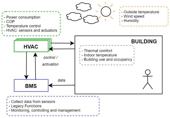
Figure 1.
Management of the building environment and the HVAC system using a BMS.
Now, through the BMS, the building data are registered and indexed in time intervals. Therefore, data from different building systems (i.e., HVAC, lighting, etc.) are treated as time series. Within this framework, HVAC data can be considered a chaotic time series since they present high volatility, nonlinearity, and nonstationarity due to the different subsystems that compose it, as well as many factors that affect the HVAC system, such as the building usage, the specifications and features of the building, the behavior of the occupant, and the weather conditions [4,6,25,62]. Even the complexity of these time series increases in buildings that have areas/zones of mixed use or activity such as theaters, offices, and shopping centers [5].
In this sense, it is necessary to build and evaluate a DL-based model that considers these temporal variations inherent to HVAC data and some external and internal factors that influence it.
3.2. Long Short-Term Memory (LSTM)
Taking into account the above, and as indicated in Section 2 (Related works), a model based on LSTM is suitable for the development of models for time series predictions, as they have a better capacity to deal with temporal dependencies as well as the detection of complex patterns, which are inherent in HVAC data in buildings [51,63]. In other words, LSTM networks have greater robustness for the handling of continuous values and present good performance with time series data of large time lags [25]. Within this context, this neural network offers a solution to the two main problems that RNNs present at the moment of learning: (i) it is not able to consider time lags far from the time series and (ii) it tends to present unstable gradients (vanishing or exploding) [4,29,55].
The LSTM network, which is an improved variant of RNN, was first introduced in 1997 by Hochreiter and Schmidhuber [27,56] and has been widely used for the analysis and prediction of time series or sequential data, such as: voice recognition, electrocardiograms, stock price, etc. [64]. This network is composed of a memory cell state denoted by and three main gates called forget gate , input gate , and output gate , as shown in Figure 2.
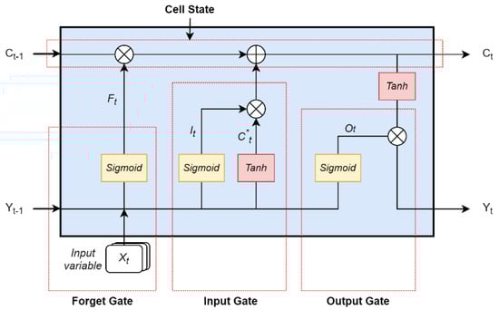
Figure 2.
Diagram of the internal structure of an LSTM network.
These gates function as valves to manage and control the information learned during training. More specifically, the forget gate determines what information to remove or keep from the memory cell; the input gate selects the information from the candidate memory cell state to update the cell state; the output gate decides the information from the memory cell so that the model only considers meaningful information to predict. The values for each of these gates are calculated according to the following equations
The memory cell and output values of the LSTM network are calculated using the following equations
where , and represent the weights and bias variables, respectively, of the three gates and the memory cell state, is the previous hidden unit information, and is the value of the current input. Thus, the use of these gates allows the LSTM network to have the ability to learn long-term dependencies in the input sequence.
Now, for the development of the LSTM-based model, we consider different data from the building BMS system. Some of these data come from the environment, HVAC system, and building. By supplying the information as a time series to the model, the model will predict the behavior and energy consumption of the building’s HVAC system. Therefore, building administrators/managers will obtain information to carry out the aforementioned intelligent strategies.
4. Methodology
In this study, we performed the procedure shown in Figure 3 to train and test the robustness of the LSTM-based DL model for forecasting the short-term (daily) energy consumption of HVAC systems in buildings. The following is a description of each of the steps involved.
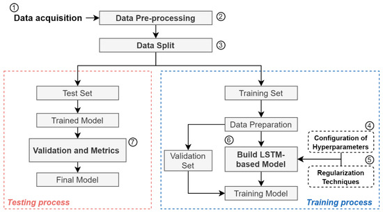
Figure 3.
Flow diagram of the model development.
4.1. Data Acquisition
We used a raw dataset from a BMS system to train and test the robustness of the model. This dataset was kindly provided by the Teatro Real of Madrid, which is the most important Spanish opera house.
The Teatro Real is a historic building built in 1850 that has an area of 65,000 m2 and a capacity for more than 1800 people. It also has several rooms for various activities and uses such as events, rehearsal rooms, studios, technical areas, and a surrounding office area.
On the other hand, this building is in operation every day of the year, with working days of 16 h (8:00 to 00:00). The HVAC system at the Teatro Real is made up of multi-HVAC subsystems [7] incorporating two chiller systems with a nominal cooling power of 350 kW and two heat pump systems with a nominal power of 195 kW for cooling and heating. These multi-HVAC subsystems are monitored and controlled by a BMS that collects data from the different sensors in the building. These data are sampled at different time intervals: one sample every 15 min (96 samples per day) for operating data from multi-HVAC subsystems and one sample every hour (24 samples per day) for internal building data. Some of the variables that the BMS of the Teatro Real keeps stored are the outside and interior temperature of the building and, relative to the multi-HVAC system, the capacity, the energy consumed, and the thermal power generated.
4.2. Data Pre-Processing
For the aforementioned case study, we performed the detection and cleaning of outliers or noisy values, since these greatly affect the precision of the predictive models [65]. For this reason, we used correlation and clustering techniques (k-means) to identify outliers.
On the other hand, the variables used for the model were indicated by the professional experts of the building, which were the following: the interior temperature of the building, the external temperature, and the energy consumed by a HVAC system. We retrieved 6912 data points distributed in each of these variables. Table 1 presents the statistics of them. For this work, the data comes from a heat pump supplied by the expert staff of the Teatro Real building. These data include the winter season since this season is the one with the highest energy consumption and cost. In addition, these data cover a longer and more uniform period of time in the thermal demand. It should be noted that this case is easily applicable to other seasons if data of the same type are provided.

Table 1.
Statistics of the variables.
In addition, in order to obtain a uniform internal temperature of the building, we considered calculating the average of this temperature recorded in the different areas, rooms, and offices of the Teatro Real in which it was influenced by the heat pump.
As a follow-up to this activity, this new variable (average internal temperature) was sampled per hour, while the other variables were sampled every 15 min. In this sense, we applied a data transformation process (subsampling) for this new variable, since it was crucial for the training of the model [66,67]. Therefore, we transformed the time interval from 1 h to 15 min., using the Piecewise Cubic Hermite Interpolating Polynomial (PCHIP) method [68,69] to equalize the resolution intervals in the Teatro Real data. It should be noted that we performed tests with the data at a 1 h resolution; however, the model lost precision when training the model due to the complexity of HVAC systems [25].
The variables used to develop a DL model are found on different scales (for example °C, kW, etc.); consequently, it was important to standardize them. From this perspective, the method we used to normalize the variables was standard normalization, also known as standard score or z-score [65].
4.3. Data Split
Once the data from the Teatro Real building had been pre-processed, we defined the forecast horizon of the energy consumption of the HVAC system in one day (short-term) since this allows for anticipating the energy that these systems will use; therefore, it will help building managers/administrators to design and implement optimal control strategies over these systems and access optimal energy rates in the continuous electricity market [8,70,71]. Therefore, the one-day forecast horizon for the building is a 96 samples/time step.
Subsequently, we divided the data into three subsets (training-set, validation-set, and testing-set) because the division of these subsets was essential for the accuracy of the model [72]. From this perspective, the pre-processed data were divided into 80% for training and 20% as unseen data to be used in the final evaluation (testing) of the model. It should be noted that 20% of the data from the training-set we used for validation during model training (see Figure 3).
Because the different variables were recorded as a time series, it is of great importance that these data sets were kept in order and preserved the temporal behavior. In addition, we had multivariate data, so it was more difficult to analyze them using classical techniques [73]. Therefore, we applied the sliding window method [72,74,75,76,77], which allows transforming time series data into supervised learning. To achieve this, the method maps the past observations (time lags) as input variables. The time lag can be 15 min., one hour, one day, or more than one day. Subsequently, it uses the time steps after this time lagged (one day of samples for the case study) as forecast output, as shown in Figure 4.
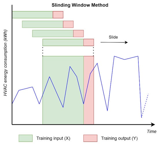
Figure 4.
Example of use of sliding window method to transform time series data to supervised learning.
It should be noted that the input variables included the three variables presented in Section 4.2. and the output was the daily energy consumption of the HVAC system to be forecasted.
4.4. Configuration of Hyperparameters
The tuning of the hyperparameters (HPs) in a DL-based model as an LSTM network has a great impact on the speed, learning capacity, and forecast accuracy of the model [27,78]. For this reason, we evaluated the model by adjusting the most relevant HPs that characterize the structure of the LSTM network, such as the activation function and number of neurons. However, before considering the HPs mentioned above, we will explain some considerations that we made with other HPs required for the training process of the model.
There are different optimizers for learning a neural network, some of which are the stochastic gradient descent (SGD), adaptive gradient algorithm (AdaGrad), Adadelta, root mean square propagation (RMSprop), and adaptive moment estimation (Adam) [29,79,80]. Although all of these optimizers perform for learning DL models, we opted for the Adam optimizer, which, according to the literature, is the most widely used for DL architectures [43] as it offers rapid convergence, a learning rate adaptive, and little tuning of HPs [81]. Similarly, batch size is a hyperparameter that determines the learning performance of the model [39,82]. It should be noted that, from the observation of performance through multiple initial training executions, it was established that the learning rate parameter was set at 0.001, batch size at 2 and the number of iterations or epochs at 50.
4.4.1. Number of Neurons
The number of neurons must be sufficient to provide the LSTM network with learning power. However, this number of neurons is selected by researchers through trial and error. Additionally, the determination of the number of neurons in the LSTM layer will depend on the application and the field in which it is to be used [83]. In this sense, we performed several preliminary tests with a number of neurons between 40 and 80 in the LSTM layer, in which we identified that between 50, 60, and 70 neurons the model performed better. Therefore, we evaluated our model with this number of neurons in the LSTM layer, to find which one best fitted our case study. Furthermore, for the output layer, the number of neurons corresponds to the one-day forecast horizon of our case study (96 neurons).
4.4.2. Activation Functions
The main purpose of the activation function is to introduce nonlinearities to the neural network [84], allowing us to model with greater certainty the nonlinear behavior or pattern typical of real-world data. Therefore, the rectified linear unit (ReLu), leaky ReLu, and exponential linear unit (ELU) activation functions, provide a good level of performance in DL-based models [29,84]. However, we must take into account the strengths and weaknesses of each of these activation functions. Below, Table 2 provides a summary of the strengths and weaknesses of each of these activation functions.
Table 2.
Strengths and weaknesses of the ReLu, ELU, Leaky ReLu activation functions.
Considering the above, each of these activation functions avoids the vanishing gradient problem; however, this is not the same with the exploding gradient problem [29,84]. For these reasons, we evaluated the following activation functions on the LSTM network:
- Hyperbolic Tangent (TanH): This activation function is shaped like an “S” similar to the sigmoid function. However, unlike the latter, which has an output value of 0 to 1, the Tanh has an output value that ranges from −1 to 1. Therefore, it allows the layer output to be normalized around zero when starting the training, helping to accelerate the convergence of the model [29].
- Scaled exponential linear unit (SeLu): This was introduced by Günter Klambauer as a variant of the exponential linear unit (ELU) [85]. An advantage of this activation function is that it performs an internal normalization (self-normalized) of the data; that is, the outputs of this function are normally distributed. Therefore, it has fast convergence and solves the problem of gradients vanishing and exploding [29,42,86].
It should be noted that we evaluated these activation functions on the input and output gates of the LSTM network. In this sense, and based on the considerations described above, Table 3 summarizes the different hyperparameters that we evaluated and used for model training.
Table 3.
Hyperparameters were evaluated and used to train the model.
4.5. Regularization Techniques
One of the challenges presented by DL-based models is overfitting. This occurs when the model is overparameterized or very complex; consequently, it learns the statistical noise from the training data, resulting in a model that overfits these data excessively. Moreover, when evaluating the model, it does not generalize correctly on the test data [29,78]. To avoid these drawbacks, we considered implementing dropout and early stopping regularization techniques.
4.5.1. Dropout
Dropout is a regularization technique applied during neural network training in a way that ignores or eliminates some neurons randomly [87]. In this way, this technique allows the neural network to be trained as if it presented a different architecture or maintained different internal connections in the layer that implements it. This means that, in each update, the network will be trained with different “forms” of the layer that maintains this regularization. The result of this process is a model that presents a higher robustness and a lower probability of overfitting to the training data [87,88]; consequently, the model is more generalizable and usable.
In addition, this technique is effective when there are limited data for training since, if there are few data, the model will fit these data and will not generalize correctly; on the other hand, if there is a large amount of data, this technique will generate a high computational cost [89].
As a follow-up to this process, we established a dropout rate of 20% since it generated good results when evaluating several executions of the model with the test.
4.5.2. Early Stopping
This technique allows network training to be regularized as soon as the model reaches a minimum threshold of the validation error of the loss function (LF) (training error metric, such as MSE or MAE). In other words, it stops training when the LF of the network increases after waiting for a number of epochs, thus providing good model generalization performance and avoiding network overfitting [29,90].
Taking into account the above, and as indicated in Section 4.3., we took 20% of the training data set as the validation-set, which allowed us to monitor and stop training when the LF did not show an improvement in the validation error. In this context, for our case study, the early stopping technique took the results obtained from LF-validation error and compared them every three epochs if there was a reduction in this error. In case this error increased after passing these three epochs, the training would stop, and the model would be selected three previous epochs before this validation error increased. An example of this can be seen in Figure 5.
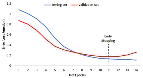
Figure 5.
Example of the early stopping regularization technique.
4.6. Build LSTM-Based Model
The architecture of the model proposed in this study for the problem of forecasting the daily energy consumption of the HVAC system in buildings is composed as follows: first, an LSTM input layer that receives all the temporal variables presented in Section 4.2. and which will be evaluated with different HPs settings (see Table 3). Second, an intermediate dropout layer will be implemented to prevent overfitting during the training. Finally, the data from this dropout layer will pass to an output layer made up of a fully-connected layer or dense layer, which will make the forecast for the next day (as shown in Figure 6). It should be noted that the weight and bias matrices were updated (learned) at each iteration during the training.
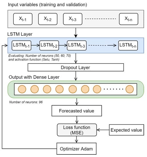
Figure 6.
Architecture proposal and training flow of the model for forecasting the daily energy consumption of the HVAC system in buildings.
Once we obtained the forecast result for the day, the actual values registered by the building BMS are compared by calculating the LF. Subsequently, the error obtained by the LF will go through Adam’s optimizer during training, which will be in charge of feedback and updating the weights of the network to minimize the LF in each epoch. Similarly, the early stopping technique will be monitored every three epochs with the validation data so that the network does not have overfitting. Therefore, the validation data follow the same architecture flow of the proposed model (see Figure 6).
4.7. Validation and Metrics
Standard DL model validation techniques such as train-test division or k-fold cross validation are not useful for evaluating and validating time series. They ignore the temporal behavior of this type of problem. For this reason, to validate our proposed model we used the Walk-Forward Validation (WFV) technique [91,92].
Taking into account the above, WFV takes the last training-set as time lagged to make a forecast; thus, it compares the output of this model with the unseen data (testing-set). Moreover, this technique allows taking different time lags to evaluate in the model; furthermore, it works well in conjunction with the sliding window method.
One of the most commonly used metrics to evaluate the performance of a forecast is MAPE since it is easy to understand and explain. However, the use of this indicator is restricted in the case of having null or close to zero measured values, which would provide undefined or very extreme values [8]. For this reason, to compare the forecasting performance of our model, we used the following metrics: coefficient of determination (R2), root mean square error (RMSE), and coefficient of variation of root mean square error (CVRMSE). It should be noted that the CVRMSE metric is especially used in this research, since the American Society of Heating, Refrigerating and Air-Conditioning Engineers (ASHRAE), the International Performance Measurement and Verification Protocol (IPMVP), and the Federal Energy Management Program (FEMP) established this indicator as a metric of the goodness of fit of a mathematical model with respect to the data or reference estimates measured in different operating conditions of an HVAC system [93,94,95,96]. Specifically, if the CVRMSE forecast error of the model is less than 0.30 it is considered valid and adequate for engineering purposes. Next, we define the equations for the error metrics
where is the number of samples, is the expected value of the i-th point,
is the mean of the expected value, and
is the predicted value.
5. Evaluations
The proposed architecture of the LSTM-based model was developed and implemented under the Python language (v3.6) using the Keras Application Programming Interface (API) (v2.4) from the open source TensorFlow library [29,97]. Additionally, the hardware in which the different tests were executed was carried out in an NVIDIA Jetson Nano Developer Kit [98].
On the other hand, the forecasts obtained were compared using different configurations that we will describe below. The architecture configuration C1 represents our proposed model applying the two regularization techniques dropout and early stopping. Configuration C2 represents the model that only applies dropout. Configuration C3 represents the model that only applies early stopping. Finally, configuration C4 represents the model without these regularization techniques.
Similarly, for all these configurations, we evaluated the different hyperparameters (HPs) shown in Table 3, where each of these HPs is labeled as follows: (S50, S60, S70) represent the SeLu activation function with 50, 60 and, 70 neurons, respectively, and (T50, T60, T70) represent the Tanh activation function with 50, 60 and, 70 neurons, respectively. In addition, we used various time lags (one to seven days), to identify the best time lag setting for the forecast of the daily (short-term) energy consumption of the building’s heat pump.
We then executed each of these configurations five times for each time lag, due to the randomness of the DNNs. Table 4, Table 5, Table 6 and Table 7 present the performance of the metrics evaluated in our study for the time lags analyzed in the different configurations of the model and HPs mentioned above. Each metric obtained is the average calculated from the executions performed.
Table 4.
Performance in the metrics evaluated when forecasting the energy consumption of the HVAC, using different time lags and HPs, applying the C1 configuration.
Table 5.
Performance in the metrics evaluated when forecasting the energy consumption of the HVAC, using different time lags and HPs, applying the C2 configuration.
Table 6.
Performance in the metrics evaluated when forecasting the energy consumption of the HVAC, using different time lags and HPs, applying the C3 configuration.
Table 7.
Performance in the metrics evaluated when forecasting the energy consumption of the HVAC, using different time lags and HPs, applying the C4 configuration.
Each of the tables presented above is divided as follows: time lags, performance metrics, and the nomenclature given for the HP sets studied. Subsequently, we analyzed the performance obtained in each of the tables and identified the best time lags, activation function, and number of neurons for each configuration, according to the evaluation metrics analyzed. The best performance obtained in Table 4, Table 5, Table 6 and Table 7 are highlighted in bold.
From this perspective, all configurations achieved good performance with time lags of seven days. Furthermore, the C1, C3, and C4 configurations performed better with a Tanh activation function of 50 neurons (T50) in the LSTM layer. C2 achieved good results with a Tanh activation function of 60 neurons (T60) in the LSTM layer.
In the same way, we carried out an in-depth analysis of the previous evidence, in which we analyzed and evaluated each configuration obtained with respect to its epochs, LF of the training-set, and LF of the validation-set, to identify the overfitting in these model configurations. In this sense, we named each configuration C1-T50, C2-T60, C3-T50, and C4-T50. Figure 7 shows each of the configurations with their values obtained for the LF, where the bar chart represents the average error of the LF (training-set and validation-set) and the red line represents the average number of epochs in which the training was completed. It should be noted that these results are the average of the five runs performed.
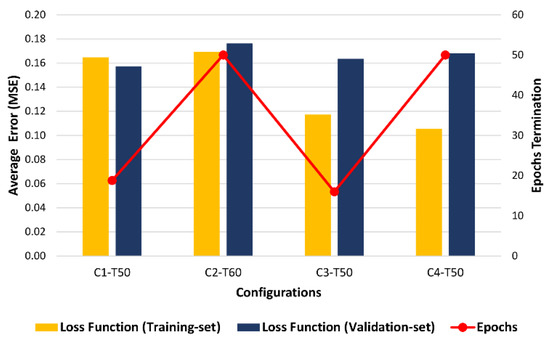
Figure 7.
Evaluation of training and validation for the best configurations obtained.
In addition, to verify the robustness and applicability of the configurations of the previously trained models, we compared the performance of the daily forecast provided by the model with respect to unseen data from the testing-set. In Figure 8, some samples are shown with the forecast of the energy consumption of the building’s heat pump obtained for one day with these configurations.
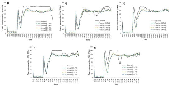
Figure 8.
Comparison of the observed values with those predicted by the configurations obtained (C1-T50, C2-T60, C3-T50, C4-T50) for the daily energy consumption of the heat pump.
For these forecasted samples, we have also evaluated and calculated the relative error of the average energy consumption and the relative error of the maximum energy consumption of the building’s heat pump. Table 8, Table 9, Table 10 and Table 11 show each configuration of the model obtained.
Table 8.
Calculation of the relative error of the daily energy consumption (average and maximum) with respect to the testing-set (model: C1-T50).
Table 9.
Calculation of the relative error of the daily energy consumption (average and maximum) with respect to the testing-set (model: C2-T60).
Table 10.
Calculation of the relative error of the daily energy consumption (average and maximum) with respect to the testing-set (model: C3-T50).
Table 11.
Calculation of the relative error of the daily energy consumption (average and maximum) with respect to the testing-set (model: C4-T50).
6. Results and Discussion
This study was developed with the objective of building a DL model based on LSTM that allows forecasting of the daily energy consumption of the HVAC system in buildings. For this, it has been applied specifically to a heat pump in a historic building, the Teatro Real in Spain. Another purpose was to evaluate the best configuration of this model by using different time lags, various HP tuning, and implementation of the dropout and early stopping regularization techniques during the training of the model.
Analyzing the performance obtained, it can be seen in Table 4, Table 5, Table 6 and Table 7, that all the configurations showed good precision in forecasting the short-term energy consumption of the building’s heat pump, given that they obtained values within the range of 0.197–0.285 of CVRMSE, the metric used by ASHRAE, IPMVP, and FEMP to validate the accuracy of a forecast model [93,94,95,96]. Although the results show that any configuration of the proposed model can be used, this does not imply that the models generalize correctly. For this reason, we analyzed and evaluated all the configurations that provided the best results in all the accuracy evaluation metrics (see Equations (7)–(9)), to identify and obtain the model with the best values of time lags, HPs tuning, and goodness of the regularization techniques.
Taking into account these considerations, as seen in Table 4, Table 5, Table 6 and Table 7, all configurations for a time lag of seven days obtained good results according to the evaluation consideration. Furthermore, for the C1, C3, and C4 configurations, better results were obtained with a Tanh activation function of 50 neurons (T50). C1 proposed configuration obtained R2, RMSE and CVRMSE values of 0.876, 18.61 and 0.205, respectively; C3 configuration obtained R2, RMSE, and CVRMSE values of 0.886, 17.88 and 0.197, respectively; C4 configuration obtained R2, RMSE, and CVRMSE values of 0.879, 18.37, and 0.202, respectively. Finally, C2 configuration obtained better results with a Tanh activation function of 60 neurons (T60), in which it achieved R2, RMSE, and CVRMSE values of 0.877, 18.56, and 0.204, respectively.
From the results shown above we can highlight several interesting findings. First, to perform a daily forecast in this case study, it was necessary to apply seven-day historical time lags. The HVAC system of a house only uses the historical behavior of the previous day to forecast the next day as there are few temporal variations throughout a week [4]. In contrast, a complex building such as the one studied here presents many disturbances during the week (e.g., occupant behavior, building use, work time, theatrical performances, events, etc.). The use of seven days of history offers the opportunity to capture these disturbances, making it feasible to anticipate the energy consumption of the HVAC system for the next day with adequate accuracy and favors the implementation of applications such as optimal control, preventive maintenance and fault detection, and diagnosis [57,58,59]. Regarding the second finding, the configurations obtained (C1-C4) achieved a good performance in the CVRMSE metric, which was between 0.095 and 0.103, less than that proposed of 0.30 by international agencies.
Other significant findings of the results obtained were the activation function and the number of neurons for the LSTM layer. In the first finding, the best results obtained using the activation function Tanh versus SeLu are highlighted. One justification for this is that, while SeLu has the ability to avoid vanishing or exploding gradient problems, it is not able to hold the gradient for a long period of time before it reaches zero, a property that Tanh can solve by calculating its second derivative [29,84,99]. In the second finding, the number of neurons evaluated in this study for the LSTM layer was 50, 60, and 70 neurons, in which three model configurations, C1, C3, and C4, performed well with only 50 neurons, whereas the C2 configuration performed better with 60 neurons.
From the previous results, we have taken the best set of configurations, including the activation function and number of neurons obtained, defined as follows: C1-T50, C2-T60, C3-T50, and C4-T50. To understand and justify the difference in the number of neurons required for the LSTM layer, we proceeded to analyze the results of the loss function (LF) and the number of epochs used by these configurations with the training-set and validation-set data.
Taking into account the above and analyzing the results observed in Figure 7, the C1-T50 configuration showed the best results with training and validation sets since the use of regularization techniques for dropout and early stopping prevented it from presenting any tendency of overfitting in LF-training and LF-validation. It is also appreciated that an average of less than 20 epochs was required to achieve good results, so this model has enough computational capacity to capture temporal variations and make a daily forecast of the energy consumption of the building´s heat pump. On the other hand, the C2-T60 configuration, although it employs a greater number of neurons and implements dropout, generated the greatest errors in LF-training and LF-validation. In addition, it had a tendency to overfit since it does not implement early stopping to monitor LF-validation during training, which continued until reaching the established maximum.
There are several possible explanations for these results: (i) the established dropout rate was not optimal for this number of neurons; (ii) the influence of other selected HPs such as learning rate, epochs, optimizer, etc. From this perspective, the use of optimization techniques focused on these HPs could improve the model accuracy [3,47,100]. Meanwhile, C3-T50 and C4-T50 configurations showed a clear trend to overfit, as LF-training decreased dramatically compared to LF-validation. On the one hand, the C3-T50 configuration, while making use of the early stopping technique, was not enough to prevent overfitting over the training-set. On the other hand, the C4-T50 configuration, by not using regularization techniques, was not able to correctly adapt to the data, causing the model to overfit. Thus, we have observed that using only the early stopping technique or any of the regularization techniques would not guarantee that the model is robust and offers good forecast accuracy in data with high temporal variation (chaotic series), as in the case of complex building HVAC systems. Therefore, the use of the early stopping technique will depend on the data, the size of the data, and the context to which it is directed.
On the other hand, to test the robustness and applicability of all the resulting C1-T50, C2-T60, C3-T50, and C4-T50 configurations, we evaluated each configuration of the model with some samples from the testing-set and obtained the corresponding daily forecasts, to compare the accuracy when making the forecast of a day, as well as determine the relative errors obtained in the forecast of the average and maximum daily energy consumption of the heat pump. In this sense, the results observed in Figure 8 show good accuracy of the configurations in the forecast and in detection of the daily temporal variation of the energy consumption of the heat pump. However, in accordance with the aforementioned results and what is observed in Table 8, Table 9, Table 10 and Table 11, the C2-T60, C3-T50, and C4-T50 configurations obtained values of the relative error of the average daily energy consumption of (7.78%, 7.80%, 7.66%) and the maximum daily energy consumption of (10.55%, 9.14%, 10.18%), respectively. The C1-T50 configuration obtained a relative error of daily average energy consumption of 7.73% and daily maximum energy consumption of 11.80%.
According to the previous results, the relative errors of the energy consumption (average and maximum) of the C2-T60, C3-T50, and C4-T50 configurations were quite low; however, this can be misleading because, by implementing one or none of the regularization techniques, these configurations cannot reliably generalize over the test-sets, as they exhibit overfitting. For the C1-T50 configuration, although the relative errors are not so low, the model could generalize better to the data since the implemented regularization techniques allowed capturing of the temporal variations.
7. Conclusions and Future Works
In this study, we developed an LSTM-based model aimed at forecasting the daily energy consumption of the HVAC system in buildings, specifically a heat pump at the Teatro Real in Spain. In particular, we focused on determining the time lags that best suits the need. In addition to identifying the best tuning of hyperparameters (HPs) for the LSTM layer, we analyzed the implementation of dropout and early stopping regularization techniques during learning the proposed model.
From this point of view, we have compared different model configurations with respect to the actual data provided by the building’s BMS, in which each model configuration implemented one, two, or none of the above regularization techniques. Subsequently, we evaluated, for all these model configurations, multiple executions of several time lags (one to seven days), with HPs as the activation function (SeLu or Tanh) and a number of 50, 60, and 70 neurons. As a result, we analyzed and evaluated the forecast accuracy of each model configuration with respect to the various results obtained in the evaluation metrics (R2, RMSE, CVRMSE).
From the experiments conducted, we identified that the CVRMSE measurement results obtained by the model configurations were within the acceptable accuracy range (<0.30) for the global uncertainty in the prediction of energy use according to the criteria indicated by the ASHRAE, IPMVP, and FEMP guidelines to validate an HVAC calibrated model [93,94,95,96]. Additionally, for all configurations, we determined that the best time lag to make a daily forecast is the previous seven days. This suggests that models aimed at forecasting the energy consumption of the HVAC system should consider a wide time lag to capture all the patterns or temporal variations of these systems and the building [5,18,26,27], so it could be a baseline for researchers studying similar complex cases.
In addition, we determined the HPs of the C1 to C4 configurations with the best performance in the metrics. The Tanh activation function was more accurate in these configurations compared with the SeLu activation function, while the best number of neurons was 50 for the C1-T50, C3-T50, and C4-T50 configurations and 60 neurons for the C2-T60 configuration. Based on this evidence, we consider that the activation functions and the number of neurons will depend on many factors, such as data size and variations, model complexity, HPs, use of regularization techniques, or the context in which it is studied. Therefore, the application of optimization techniques for some of these factors would improve the accuracy for model prediction [3], although this would imply a high computational cost [36,62].
We also observed that dropout and early stopping regularization techniques can work together in analogous scenarios, as they easily capture volatility, nonlinearity, and hidden patterns during DNN training. In fact, we have demonstrated that the configuration of model C1-T50, which implemented these regularization techniques, was able to determine the relative error of the forecast of average and maximum daily energy consumption by 7.73% and 11.80%, respectively. In addition, this model has a lower performance in the CVRMSE metric of 0.095 than that proposed by the ASHRAE, IPMVP, and FEMP guidelines. Therefore, it generates generalizable forecasts and is capable of capturing the temporal variations of a complex building such as the one studied.
Taking into account the above, this HVAC system energy consumption forecast model could be part of a broader framework, in which, through the analysis of the forecast generated, intelligent decisions can be made, such as performing preventive maintenance, fault detection and diagnosis, optimization of operation modes, etc.
On the other hand, it should be noted that the proposed model can be improved by adjusting other HPs, such as the learning rate, optimizer type, number of epochs, dropout rate, and number of delay or “patience” for early stopping. Therefore, it would be interesting to investigate whether there is an improvement in the forecasting accuracy of the model when tuning some of these HPs [4,62].
Finally, in future work, we will compare the performance of this model with respect to other Deep Learning models, under the implementation of an intelligent microservices environment within a cloud-connected ecosystem, in order to improve the BMS architecture and extend its functionalities [32] since microservices allow the decoupling of services that require higher computational power (GPU or parallel computing) [101].
Author Contributions
Conceptualization, J.M.G.-P. and M.V.-L.; Methodology, L.M.-P., H.C.-G., J.M.G.-P. and M.V.-L.; Software, L.M.-P. and H.C.-G.; Validation, L.M.-P., J.M.G.-P., M.V.-L., C.S.d.B. and J.L.C.-S.; Formal analysis, L.M.-P., J.M.G.-P., M.V.-L. and J.L.C.-S.; Investigation, L.M.-P., H.C.-G. and J.M.G.-P.; Data curation, L.M.-P., H.C.-G. and J.M.G.-P.; Writing—original draft preparation, L.M.-P., H.C.-G., J.M.G.-P. and M.V.-L.; Writing—review and editing, L.M.-P., H.C.-G., J.M.G.-P. and M.V.-L.; Visualization, L.M.-P., H.C.-G. and J.L.C.-S.; Supervision, J.M.G.-P. and M.V.-L.; Project administration, J.M.G.-P. and C.S.d.B.; Funding acquisition, J.M.G.-P. and C.S.d.B. All authors have read and agreed to the published version of the manuscript.
Funding
This study forms part of the “Smart Energy” Campus of International Excellence (CIE), promoted by the Universidad de Alcalá and the Universidad Rey Juan Carlos, for the financial support received by granting the authors the Second prize of the 2019 Awards Call for the research project: “Intelligent Management System for Optimizing Energy Consumption in Building Air Conditioning”. In addition, this work forms part of the project “Smart Tool for the Design of Residential Projects and Energetically Sustainable Buildings project” funding from the FONDO I + D + I SENACYT, 2018.
Institutional Review Board Statement
Not applicable.
Informed Consent Statement
Not applicable.
Data Availability Statement
Data sharing is not applicable to this article.
Acknowledgments
We would like to extend special thanks to the management committee of Teatro Real (Madrid, Spain) who contributed with the dataset of the building HVAC System. In addition, we would like to thank the company “ACIX ENERGIA Y MEDIO AMBIENTE S.L.” for his technical-scientific advice on the concepts related to HVAC systems in singular buildings. Finally, we thank the National Secretariat for Science, Technology and Innovation (SENACYT, Panama) and the Institute for the Training and Use of Human Resources (IFARHU), for the doctoral study scholarship awarded within the IFARHU-SENACYT doctoral scholarship program, 2018.
Conflicts of Interest
The authors declare no conflict of interest.
Nomenclature
| Acronyms | Description |
| HVAC | Heating, ventilating, and air conditioning |
| BMS | Building management system |
| ML | Machine learning |
| DL | Deep learning |
| DNN | Deep neural network |
| LSTM | Long short-term memory |
| RNN | Recurrent neural network |
| MLR | Multiple-linear regression |
| ARIMA | Autoregressive integrated moving average |
| DT | Decision Tree |
| RF | Random Forest |
| SVM | Support vector machine |
| ANN | Artificial neural network |
| MLP | Multilayer perceptron |
| HPs | Hyperparameters |
| SGD | Stochastic gradient descent |
| AdaGrad | Adaptive gradient algorithm |
| RMSprop | Root mean square propagation |
| Adam | Adaptive moment estimation |
| ReLu | Rectified linear unit |
| Leaky ReLu | Leaky rectified linear unit |
| ELU | Exponential linear unit |
| SeLu | Scaled exponential linear unit |
| Tanh | Hyperbolic tangent |
| LF | Loss function |
| MSE | Mean squared error |
| MAE | Mean absolute error |
| MAPE | Mean average percentage error |
| WFV | Walk-forward validation |
| R2 | Coefficient of determination |
| RMSE | Root mean square error |
| CVRMSE | Coefficient of variation of root mean square error |
| ASHRAE | American Society of Heating, Refrigerating and Air-Conditioning Engineers |
| IPMVP | International Performance Measurement and Verification Protocol |
| FEMP | Federal Energy Management Program |
References
- Burcin, B.-G.; Ioannis, B.; Omar, E.-A.; Nora, E.-G.; Tarek, M.; Shuai, L. Civil Engineering Grand Challenges: Opportunities for Data Sensing, Information Analysis, and Knowledge Discovery. J. Comput. Civ. Eng. 2014, 28, 4014013. [Google Scholar] [CrossRef]
- European Commission. Energy Performance of Buildings Directive. Available online: https://ec.europa.eu/energy/topics/energy-efficiency/energy-efficient-buildings/energy-performance-buildings-directive_en (accessed on 7 March 2021).
- Hwang, J.K.; Yun, G.Y.; Lee, S.; Seo, H.; Santamouris, M. Using deep learning approaches with variable selection process to predict the energy performance of a heating and cooling system. Renew. Energy 2020, 149, 1227–1245. [Google Scholar] [CrossRef]
- Sendra-Arranz, R.; Gutiérrez, A. A long short-term memory artificial neural network to predict daily HVAC consumption in buildings. Energy Build. 2020, 216, 109952. [Google Scholar] [CrossRef]
- Yildiz, B.; Bilbao, J.I.; Sproul, A.B. A review and analysis of regression and machine learning models on commercial building electricity load forecasting. Renew. Sustain. Energy Rev. 2017, 73, 1104–1122. [Google Scholar] [CrossRef]
- Kusiak, A.; Xu, G. Modeling and optimization of HVAC systems using a dynamic neural network. Energy 2012, 42, 241–250. [Google Scholar] [CrossRef]
- Aguilar, J.; Garcés-Jiménez, A.; Gallego-Salvador, N.; Gutiérrez de Mesa, J.A.; Gomez-Pulido, J.M.; García-Tejedor, Á.J. Autonomic Management Architecture for Multi-HVAC systems in Smart Buildings. IEEE Access 2019, 7, 123402–123415. [Google Scholar] [CrossRef]
- Sun, Y.; Haghighat, F.; Fung, B.C.M. A review of the-state-of-the-art in data-driven approaches for building energy prediction. Energy Build. 2020, 221, 110022. [Google Scholar] [CrossRef]
- Spandagos, C.; Ng, T.L. Equivalent full-load hours for assessing climate change impact on building cooling and heating energy consumption in large Asian cities. Appl. Energy 2017, 189, 352–368. [Google Scholar] [CrossRef]
- Mocanu, E.; Nguyen, P.H.; Gibescu, M.; Kling, W.L. Deep learning for estimating building energy consumption. Sustain. Energy Grids Netw. 2016, 6, 91–99. [Google Scholar] [CrossRef]
- Kuster, C.; Rezgui, Y.; Mourshed, M. Electrical load forecasting models: A critical systematic review. Sustain. Cities Soc. 2017, 35, 257–270. [Google Scholar] [CrossRef]
- Gonzalez-Romera, E.; Jaramillo-Moran, M.A.; Carmona-Fernandez, D. Monthly Electric Energy Demand Forecasting Based on Trend Extraction. IEEE Trans. Power Syst. 2006, 21, 1946–1953. [Google Scholar] [CrossRef]
- Friedrich, L.; Afshari, A. Short-term Forecasting of the Abu Dhabi Electricity Load Using Multiple Weather Variables. Energy Procedia 2015, 75, 3014–3026. [Google Scholar] [CrossRef] [Green Version]
- Ahmad, T.; Chen, H.; Guo, Y.; Wang, J. A comprehensive overview on the data driven and large scale based approaches for forecasting of building energy demand: A review. Energy Build. 2018, 165, 301–320. [Google Scholar] [CrossRef]
- Mohandes, S.R.; Zhang, X.; Mahdiyar, A. A comprehensive review on the application of artificial neural networks in building energy analysis. Neurocomputing 2019, 340, 55–75. [Google Scholar] [CrossRef]
- Chou, J.-S.; Ngo, N.-T. Time series analytics using sliding window metaheuristic optimization-based machine learning system for identifying building energy consumption patterns. Appl. Energy 2016, 177, 751–770. [Google Scholar] [CrossRef]
- Deb, C.; Zhang, F.; Yang, J.; Lee, S.E.; Shah, K.W. A review on time series forecasting techniques for building energy consumption. Renew. Sustain. Energy Rev. 2017, 74, 902–924. [Google Scholar] [CrossRef]
- Amasyali, K.; El-Gohary, N.M. A review of data-driven building energy consumption prediction studies. Renew. Sustain. Energy Rev. 2018, 81, 1192–1205. [Google Scholar] [CrossRef]
- Bourdeau, M.; Zhai, X.Q.; Nefzaoui, E.; Guo, X.; Chatellier, P. Modeling and forecasting building energy consumption: A review of data-driven techniques. Sustain. Cities Soc. 2019, 48, 101533. [Google Scholar] [CrossRef]
- Liu, T.; Xu, C.; Guo, Y.; Chen, H. A novel deep reinforcement learning based methodology for short-term HVAC system energy consumption prediction. Int. J. Refrig. 2019, 107, 39–51. [Google Scholar] [CrossRef]
- Shao, X.; Pu, C.; Zhang, Y.; Kim, C.S. Domain Fusion CNN-LSTM for Short-Term Power Consumption Forecasting. IEEE Access 2020, 8, 188352–188362. [Google Scholar] [CrossRef]
- Fan, C.; Xiao, F.; Wang, S. Development of prediction models for next-day building energy consumption and peak power demand using data mining techniques. Appl. Energy 2014, 127, 1–10. [Google Scholar] [CrossRef]
- Seyedzadeh, S.; Rahimian, F.P.; Glesk, I.; Roper, M. Machine learning for estimation of building energy consumption and performance: A review. Vis. Eng. 2018, 6. [Google Scholar] [CrossRef]
- Chou, J.-S.; Truong, D.-N. Multistep energy consumption forecasting by metaheuristic optimization of time-series analysis and machine learning. Int. J. Energy Res. 2021, 45, 4581–4612. [Google Scholar] [CrossRef]
- Zhou, C.; Fang, Z.; Xu, X.; Zhang, X.; Ding, Y.; Jiang, X.; Ji, Y. Using long short-term memory networks to predict energy consumption of air-conditioning systems. Sustain. Cities Soc. 2020, 55, 102000. [Google Scholar] [CrossRef]
- Walter, T.; Price, P.N.; Sohn, M.D. Uncertainty estimation improves energy measurement and verification procedures. Appl. Energy 2014, 130, 230–236. [Google Scholar] [CrossRef] [Green Version]
- Somu, N.; Raman M R, G.; Ramamritham, K. A hybrid model for building energy consumption forecasting using long short term memory networks. Appl. Energy 2020, 261, 114131. [Google Scholar] [CrossRef]
- Zhang, C.; Li, J.; Zhao, Y.; Li, T.; Chen, Q.; Zhang, X. A hybrid deep learning-based method for short-term building energy load prediction combined with an interpretation process. Energy Build. 2020, 225, 110301. [Google Scholar] [CrossRef]
- Géron, A. Hands-on Machine Learning with Scikit-Learn, Keras, and TensorFlow: Concepts, Tools, and Techniques to Build Intelligent Systems; O’Reilly Media: Newton, MA, USA, 2019; ISBN 1492032611. [Google Scholar]
- Proyecto CEI “Energía Inteligente”. Available online: https://www.campusenergiainteligente.es/en/ (accessed on 7 April 2021).
- Mendoza-Pittí, L.; Garcés-Jiménez, A.; Aguilar, J.; Gómez-Pulido, J.M.; Vargas-Lombardo, M. Proposal of Physical Models of Multi-HVAC Systems for Energy Efficiency in Smart Buildings. In Proceedings of the 2019 7th International Engineering, Sciences and Technology Conference (IESTEC), Panama, Panama, 9–11 October 2019; pp. 641–646. [Google Scholar]
- Mendoza-Pitti, L.; Calderón-Gómez, H.; Vargas-Lombardo, M.; Gómez-Pulido, J.M.; Castillo-Sequera, J.L. Towards a Service-Oriented Architecture for the Energy Efficiency of Buildings: A Systematic Review. IEEE Access 2021, 9, 26119–26137. [Google Scholar] [CrossRef]
- Aguilar, J.; Garcés-Jiménez, A.; Gómez-Pulido, J.M.; R-Moreno, M.D.; Gutiérrez-de-Mesa, J.-A.; Gallego, N. Autonomic Management of a Building’s multi-HVAC System Start-Up. IEEE Access 2021. [Google Scholar] [CrossRef]
- Le Cun, Y.; Bengio, Y.; Hinton, G. Deep learning. Nature 2015, 521, 436–444. [Google Scholar] [CrossRef]
- Mabrouk, A.; Redondo, R.P.D.; Kayed, M. Deep Learning-Based Sentiment Classification: A Comparative Survey. IEEE Access 2020, 8, 85616–85638. [Google Scholar] [CrossRef]
- Torres, J.F.; Hadjout, D.; Sebaa, A.; Martínez-Álvarez, F.; Troncoso, A. Deep Learning for Time Series Forecasting: A Survey. Big Data 2020, 9, 3–21. [Google Scholar] [CrossRef]
- Elhariri, E.; Taie, S.A. H-Ahead Multivariate microclimate Forecasting System Based on Deep Learning. In Proceedings of the 2019 International Conference on Innovative Trends in Computer Engineering (ITCE), Aswan, Egypt, 2–4 February 2019; pp. 168–173. [Google Scholar]
- Chandramitasari, W.; Kurniawan, B.; Fujimura, S. Building Deep Neural Network Model for Short Term Electricity Consumption Forecasting. In Proceedings of the 2018 International Symposium on Advanced Intelligent Informatics (SAIN), Yogyakarta, Indonesia, 29–30 August 2018; pp. 43–48. [Google Scholar]
- Hadri, S.; Naitmalek, Y.; Najib, M.; Bakhouya, M.; Fakhri, Y.; Elaroussi, M. A Comparative Study of Predictive Approaches for Load Forecasting in Smart Buildings. In Proceedings of the Procedia Computer Science, Coimbra, Portugal, 4–7 November 2019; Volume 160, pp. 173–180. [Google Scholar]
- Kim, T.-Y.; Cho, S.-B. Predicting residential energy consumption using CNN-LSTM neural networks. Energy 2019, 182, 72–81. [Google Scholar] [CrossRef]
- Alden, R.E.; Gong, H.; Ababei, C.; Ionel, D.M. LSTM Forecasts for Smart Home Electricity Usage. In Proceedings of the 2020 9th International Conference on Renewable Energy Research and Application (ICRERA), Glasgow, UK, 27–30 September 2020; pp. 434–438. [Google Scholar]
- Moon, J.; Park, S.; Rho, S.; Hwang, E. A comparative analysis of artificial neural network architectures for building energy consumption forecasting. Int. J. Distrib. Sens. Netw. 2019, 15. [Google Scholar] [CrossRef] [Green Version]
- Rahman, A.; Srikumar, V.; Smith, A.D. Predicting electricity consumption for commercial and residential buildings using deep recurrent neural networks. Appl. Energy 2018, 212, 372–385. [Google Scholar] [CrossRef]
- Alawadi, S.; Mera, D.; Fernández-Delgado, M.; Alkhabbas, F.; Olsson, C.M.; Davidsson, P. A comparison of machine learning algorithms for forecasting indoor temperature in smart buildings. Energy Syst. 2020. [Google Scholar] [CrossRef] [Green Version]
- Kim, Y.; Son, H.; Kim, S. Short term electricity load forecasting for institutional buildings. Energy Rep. 2019, 5, 1270–1280. [Google Scholar] [CrossRef]
- Kuo, P.-H.; Huang, C.-J. A High Precision Artificial Neural Networks Model for Short-Term Energy Load Forecasting. Energies 2018, 11, 213. [Google Scholar] [CrossRef] [Green Version]
- Kumar, S.; Hussain, L.; Banarjee, S.; Reza, M. Energy Load Forecasting using Deep Learning Approach-LSTM and GRU in Spark Cluster. In Proceedings of the 2018 Fifth International Conference on Emerging Applications of Information Technology (EAIT), Kolkata, India, 12–13 January 2018; pp. 1–4. [Google Scholar]
- Fan, C.; Wang, J.; Gang, W.; Li, S. Assessment of deep recurrent neural network-based strategies for short-term building energy predictions. Appl. Energy 2019, 236, 700–710. [Google Scholar] [CrossRef]
- Wang, L.; Lee, E.W.M.; Yuen, R.K.K. Novel dynamic forecasting model for building cooling loads combining an artificial neural network and an ensemble approach. Appl. Energy 2018, 228, 1740–1753. [Google Scholar] [CrossRef]
- Roy, S.S.; Samui, P.; Nagtode, I.; Jain, H.; Shivaramakrishnan, V.; Mohammadi-ivatloo, B. Forecasting heating and cooling loads of buildings: A comparative performance analysis. J. Ambient Intell. Humaniz. Comput. 2020, 11, 1253–1264. [Google Scholar] [CrossRef]
- Cho, J.S.; Hu, Z.; Sartipi, M. A/C Load Forecasting Using Deep Learning. In Proceedings of the 2017 International Conference on Computational Science and Computational Intelligence (CSCI), Las Vegas, NV, USA, 14–16 December 2017; pp. 1840–1841. [Google Scholar]
- Machida, Y.; Honoki, H.; Kawano, H.; Sato, F.; Ishikawa, J. Power Consumption Estimation for Building Air Conditioning Systems Using Recurrent Neural Network. In Proceedings of the 2020 IEEE/SICE International Symposium on System Integration (SII), Honolulu, HI, USA, 12–15 January 2020; pp. 854–861. [Google Scholar]
- Ellis, M.J.; Chinde, V. An encoder–decoder LSTM-based EMPC framework applied to a building HVAC system. Chem. Eng. Res. Des. 2020, 160, 508–520. [Google Scholar] [CrossRef]
- Hwang, I.; Cho, H.; Ji, Y.; Kim, H. Estimating Power Consumption of Air-conditioners Using a Sequence-to-sequence Model. In Proceedings of the 2019 IEEE 9th International Conference on Consumer Electronics (ICCE-Berlin), Berlin, Germany, 8–11 September 2019; pp. 295–300. [Google Scholar]
- Mtibaa, F.; Nguyen, K.-K.; Azam, M.; Papachristou, A.; Venne, J.-S.; Cheriet, M. LSTM-based indoor air temperature prediction framework for HVAC systems in smart buildings. Neural Comput. Appl. 2020, 32, 17569–17585. [Google Scholar] [CrossRef]
- Hochreiter, S.; Schmidhuber, J. Long Short-Term Memory. Neural Comput. 1997, 9, 1735–1780. [Google Scholar] [CrossRef] [PubMed]
- Jeong, J.; Hong, T.; Ji, C.; Kim, J.; Lee, M.; Jeong, K.; Koo, C. Development of a prediction model for the cost saving potentials in implementing the building energy efficiency rating certification. Appl. Energy 2017, 189, 257–270. [Google Scholar] [CrossRef]
- Gao, D.; Sun, Y.; Lu, Y. A robust demand response control of commercial buildings for smart grid under load prediction uncertainty. Energy 2015, 93, 275–283. [Google Scholar] [CrossRef]
- Xue, X.; Wang, S.; Sun, Y.; Xiao, F. An interactive building power demand management strategy for facilitating smart grid optimization. Appl. Energy 2014, 116, 297–310. [Google Scholar] [CrossRef]
- Qian, F.; Gao, W.; Yang, Y.; Yu, D. Potential analysis of the transfer learning model in short and medium-term forecasting of building HVAC energy consumption. Energy 2020, 193, 116724. [Google Scholar] [CrossRef]
- Pérez-Lombard, L.; Ortiz, J.; Pout, C. A review on buildings energy consumption information. Energy Build. 2008, 40, 394–398. [Google Scholar] [CrossRef]
- Almalaq, A.; Zhang, J.J. Evolutionary Deep Learning-Based Energy Consumption Prediction for Buildings. IEEE Access 2019, 7, 1520–1531. [Google Scholar] [CrossRef]
- Mellouli, N.; Akerma, M.; Hoang, M.; Leducq, D.; Delahaye, A. Deep Learning Models for Time Series Forecasting of Indoor Temperature and Energy Consumption in a Cold Room. In Computational Collective Intelligence; Nguyen, N.T., Chbeir, R., Exposito, E., Aniorté, P., Trawiński, B., Eds.; Springer International Publishing: Cham, Switzerland, 2019; pp. 133–144. ISBN 978-3-030-28374-2. [Google Scholar]
- Yu, Y.; Si, X.; Hu, C.; Zhang, J. A Review of Recurrent Neural Networks: LSTM Cells and Network Architectures. Neural Comput. 2019, 31, 1235–1270. [Google Scholar] [CrossRef] [PubMed]
- Zhu, J.; Ge, Z.; Song, Z.; Gao, F. Review and big data perspectives on robust data mining approaches for industrial process modeling with outliers and missing data. Annu. Rev. Control 2018, 46, 107–133. [Google Scholar] [CrossRef]
- Pal, B.; Tarafder, A.K.; Rahman, M.S. Synthetic Samples Generation for Imbalance Class Distribution with LSTM Recurrent Neural Networks. In Proceedings of the International Conference on Computing Advancements; Association for Computing Machinery, New York, NY, USA, 10–12 January 2020; pp. 1–5. [Google Scholar]
- Chawla, N.V.; Lazarevic, A.; Hall, L.O.; Bowyer, K.W. SMOTEBoost: Improving Prediction of the Minority Class in Boosting. In European Conference on Principles of Data Mining and Knowledge Discovery; Lavrač, N., Gamberger, D., Todorovski, L., Blockeel, H., Eds.; Springer Berlin Heidelberg: Berlin/Heidelberg, Germany, 2003; pp. 107–119. [Google Scholar]
- Lepot, M.; Aubin, J.-B.; Clemens, F.H.L.R. Interpolation in Time Series: An Introductive Overview of Existing Methods, Their Performance Criteria and Uncertainty Assessment. Water 2017, 9, 796. [Google Scholar] [CrossRef] [Green Version]
- Fritsch, F.N.; Carlson, R.E. Monotone Piecewise Cubic Interpolation. SIAM J. Numer. Anal. 1980, 17, 238–246. [Google Scholar] [CrossRef]
- Panapongpakorn, T.; Banjerdpongchai, D. Short-Term Load Forecast for Energy Management Systems Using Time Series Analysis and Neural Network Method with Average True Range. In Proceedings of the 2019 First International Symposium on Instrumentation, Control, Artificial Intelligence, and Robotics (ICA-SYMP), Bangkok, Thailand, 16–18 January 2019; pp. 86–89. [Google Scholar]
- Chou, J.-S.; Tran, D.-S. Forecasting energy consumption time series using machine learning techniques based on usage patterns of residential householders. Energy 2018, 165, 709–726. [Google Scholar] [CrossRef]
- Chae, Y.T.; Horesh, R.; Hwang, Y.; Lee, Y.M. Artificial neural network model for forecasting sub-hourly electricity usage in commercial buildings. Energy Build. 2016, 111, 184–194. [Google Scholar] [CrossRef]
- Tsay, R.S. Multivariate Time Series Analysis: With R and Financial Applications; John Wiley & Sons: Hoboken, NJ, USA, 2013. [Google Scholar]
- Vafaeipour, M.; Rahbari, O.; Rosen, M.A.; Fazelpour, F.; Ansarirad, P. Application of sliding window technique for prediction of wind velocity time series. Int. J. Energy Environ. Eng. 2014, 5, 105. [Google Scholar] [CrossRef] [Green Version]
- Paoli, C.; Voyant, C.; Muselli, M.; Nivet, M.-L. Forecasting of preprocessed daily solar radiation time series using neural networks. Sol. Energy 2010, 84, 2146–2160. [Google Scholar] [CrossRef] [Green Version]
- Gasparin, A.; Lukovic, S.; Alippi, C. Deep learning for time series forecasting: The electric load case. arXiv 2019, arXiv:1907.09207. [Google Scholar]
- Somu, N.; Raman M R, G.; Ramamritham, K. A deep learning framework for building energy consumption forecast. Renew. Sustain. Energy Rev. 2021, 137, 110591. [Google Scholar] [CrossRef]
- Rätz, M.; Javadi, A.P.; Baranski, M.; Finkbeiner, K.; Müller, D. Automated data-driven modeling of building energy systems via machine learning algorithms. Energy Build. 2019, 202, 109384. [Google Scholar] [CrossRef]
- Choi, D.; Shallue, C.J.; Nado, Z.; Lee, J.; Maddison, C.J.; Dahl, G.E. On empirical comparisons of optimizers for deep learning. arXiv 2019, arXiv:1910.05446. [Google Scholar]
- Okewu, E.; Adewole, P.; Sennaike, O. Experimental Comparison of Stochastic Optimizers in Deep Learning. In Proceedings of the Computational Science and Its Applications—ICCSA 2019, Saint Petersburg, Russia, 1–4 July 2019; Misra, S., Gervasi, O., Murgante, B., Stankova, E., Korkhov, V., Torre, C., Rocha, A.M.A.C., Taniar, D., Apduhan, B.O., Tarantino, E., Eds.; Springer International Publishing: Cham, Switzerland, 2019; pp. 704–715. [Google Scholar]
- Kingma, D.P.; Ba, J. Adam: A method for stochastic optimization. In Proceedings of the 3rd International Conference on Learning Representations (ICLR), San Diego, CA, USA, 7–9 May 2015. [Google Scholar]
- Abbasimehr, H.; Shabani, M.; Yousefi, M. An optimized model using LSTM network for demand forecasting. Comput. Ind. Eng. 2020, 143, 106435. [Google Scholar] [CrossRef]
- Hu, Y.-L.; Chen, L. A nonlinear hybrid wind speed forecasting model using LSTM network, hysteretic ELM and Differential Evolution algorithm. Energy Convers. Manag. 2018, 173, 123–142. [Google Scholar] [CrossRef]
- Rasamoelina, A.D.; Adjailia, F.; Sinčák, P. A Review of Activation Function for Artificial Neural Network. In Proceedings of the 2020 IEEE 18th World Symposium on Applied Machine Intelligence and Informatics (SAMI), Herlany, Slovakia, 23–25 January 2020; pp. 281–286. [Google Scholar]
- Klambauer, G.; Unterthiner, T.; Mayr, A.; Hochreiter, S. Self-normalizing neural networks. In Proceedings of the Advances in Neural InformationProcessing Systems (NIPS), Long Beach, CA, USA, 4–9 December 2017; Curran Associates Inc.: Long Beach, CA, USA; pp. 972–981. [Google Scholar]
- Kuan, L.; Yan, Z.; Xin, W.; Yan, C.; Xiangkun, P.; Wenxue, S.; Zhe, J.; Yong, Z.; Nan, X.; Xin, Z. Short-term electricity load forecasting method based on multilayered self-normalizing GRU network. In Proceedings of the 2017 IEEE Conference on Energy Internet and Energy System Integration (EI2), Beijing, China, 26–28 November 2017; pp. 1–5. [Google Scholar]
- Srivastava, N.; Hinton, G.; Krizhevsky, A.; Sutskever, I.; Salakhutdinov, R. Dropout: A simple way to prevent neural networks from overfitting. J. Mach. Learn. Res. 2014, 15, 1929–1958. [Google Scholar]
- Aggarwal, C.C. Teaching Deep Learners to Generalize BT—Neural Networks and Deep Learning: A Textbook; Aggarwal, C.C., Ed.; Springer International Publishing: Cham, Switzerland, 2018; pp. 169–216. ISBN 978-3-319-94463-0. [Google Scholar]
- Goodfelow, I.; Bengio, Y.; Courville, A. Deep Learning (Adaptive Computation and Machine Learning Series); MIT Press: Cambridge, MA, USA, 2016; Volume 10. [Google Scholar]
- Aggarwal, C.C. An Introduction to Neural Networks BT—Neural Networks and Deep Learning: A Textbook; Aggarwal, C.C., Ed.; Springer International Publishing: Cham, Switzerland, 2018; pp. 1–52. ISBN 978-3-319-94463-0. [Google Scholar]
- Bergmeir, C.; Benítez, J.M. On the use of cross-validation for time series predictor evaluation. Inf. Sci. 2012, 191, 192–213. [Google Scholar] [CrossRef]
- Udeh, K.; Wanik, D.W.; Bassill, N.; Anagnostou, E. Time Series Modeling of Storm Outages with Weather Mesonet Data for Emergency Preparedness and Response. In Proceedings of the 2019 IEEE 10th Annual Ubiquitous Computing, Electronics & Mobile Communication Conference (UEMCON), New York, NY, USA, 10–12 October 2019; pp. 499–505. [Google Scholar]
- ASHRAE. ASHRAE Guideline 14-2014—Measurement of Energy, Demand and Water Savings; American Society of Heating, Refrigeration and Air Conditioning Engineers: Atlanta, GA, USA, 2014. [Google Scholar]
- Runge, J.; Zmeureanu, R. Forecasting Energy Use in Buildings Using Artificial Neural Networks: A Review. Energies 2019, 12, 3254. [Google Scholar] [CrossRef] [Green Version]
- ASHRAE. Ashrae Guideline 14: Measurement of Energy and Demand Savings; American Society of Heating, Refrigeration and Air Conditioning Engineers: Atlanta, GA, USA, 2002; Volume 35. [Google Scholar]
- Ruiz, G.R.; Bandera, C.F. Validation of Calibrated Energy Models: Common Errors. Energies 2017, 10, 1587. [Google Scholar] [CrossRef] [Green Version]
- Chollet, F. Others Keras. 2015. Available online: https://keras.io (accessed on 5 April 2021).
- Dustin, F. Jetson Nano Brings AI Computing to Everyone. Available online: https://developer.nvidia.com/blog/jetson-nano-ai-computing/ (accessed on 5 April 2021).
- Sarowar, G.; Naser, M.; Nizamuddin, S.M.; Imtiaz Bin Hamid, N.; Mahmud, A. Enhancing Bengali character recognition process applying heuristics on Neural Network. Int. J. Comput. Sci. Netw. Secur. 2009, 9, 154. [Google Scholar]
- Djenouri, D.; Laidi, R.; Djenouri, Y.; Balasingham, I. Machine Learning for Smart Building Applications: Review and Taxonomy. ACM Comput. Surv. 2019, 52. [Google Scholar] [CrossRef]
- Calderon-Gomez, H.; Mendoza-Pitti, L.; Vargas-Lombardo, M.; Gomez-Pulido, J.M.; Castillo-Sequera, J.L.; Sanz-Moreno, J.; Sencion, G. Telemonitoring System for Infectious Disease Prediction in Elderly People Based on a Novel Microservice Architecture. IEEE Access 2020, 8, 118340–118354. [Google Scholar] [CrossRef]
Publisher’s Note: MDPI stays neutral with regard to jurisdictional claims in published maps and institutional affiliations. |
© 2021 by the authors. Licensee MDPI, Basel, Switzerland. This article is an open access article distributed under the terms and conditions of the Creative Commons Attribution (CC BY) license (https://creativecommons.org/licenses/by/4.0/).