1. Introduction
Sports forecasting research has developed rapidly in recent years and begun to cover different sports, methods, and research questions. Previous studies from various disciplines have extensively investigated various predictive aspects of sports match outcomes. Several review articles [
1,
2,
3,
4,
5,
6,
7] have synthesized and organized existing predictive models with different perspectives based on human heuristics, quantitative models, ratings and rankings, betting odds, machine learning, and hybrid methods and compared their prediction capabilities.
For sports betting, which is a billion-dollar industry, accurate predictive models are necessary to set the baseline for betting odds [
8,
9]. Given that an improper setting of betting odds will bring huge losses to betting companies, the win/loss predictions implied in the odds are highly credible. Therefore, these odds are frequently adopted by researchers in economic and financial contexts and manipulated via a time series method to examine efficiency [
10,
11], study irrational behavior [
12], and predict wins–losses [
13,
14] in betting markets. However, such odds-based models mostly focus on how to beat bookmakers and measure performance based on the returns obtained from the predicted outcome in conjunction with the betting strategy [
15], not pursuing the accuracy of the predictions [
16].
Similar to assessing risky financial market behavior, sports competition outcome predictions are assessed based on systemic and non-systemic effects [
7]. Systematic effects are mainly related to the strength of teams, whereas non-systematic effects are some random factors. In general, systematic effects are relatively mature to analyze. By using the past performance of each team, various quality measures for teams or players and statistical-based metrics for building prediction models have been introduced. Experienced practitioners often use heuristics to measure the strengths and weaknesses of teams and to determine the winner of a match. By contrast, non-systematic effects are usually difficult to predict. Some predictive models that have been comprehensively tested and applied in stock markets over the past decade, such as stochastic processes, probability distribution models, and Monte Carlo simulations, have also been applied in sports forecasting.
However, some scholars argue that stock price fluctuations do not completely follow the stochastic process but rather show preceding and succeeding relationships that highlight behavioral patterns. Consequently, the behavioral patterns of these relationships have been widely explored in recent years through pattern recognition based on technical indicator analyses and knowledge graphs, such as candlesticks for prediction modeling. Candlesticks can clearly show the degree of fluctuation and are commonly used in stock market analysis and prediction, as well as in a few novel studies for the prediction of teens’ stress level change on a micro-blog platform [
17], prediction of air quality changes [
18], analysis of the teaching model effectiveness [
19], and prediction of sports match outcomes [
20]. While the results of sports games are traditionally considered independent events that do not affect one another, some scholars have recently proposed that these games are not entirely independent events and that certain trends or regularities may occur as a result of previous events [
6]. Some scholars have also suggested to exclude many factors that affect winning and losing, and considered only the scores and the match results as the raw data, using the score-driven time series to build prediction model of football match outcomes [
21,
22] In addition, in professional sports with intensive schedules, a win or loss in the previous match can bring anxiety for the player and generate a certain impact on the next match, such as the “hot hand” effect [
23,
24]. Therefore, behavioral patterns may exist in sports matches. Similar to the stock market behavior resulting from the psychological reaction of the investing public, the behavior of a sports team is influenced by the psychological reaction of several players. In team sports, the outcome of a match is easily influenced by the main powerful player on the field and can greatly vary across each player [
25]. Identifying these implicit behavioral patterns of sports remains extremely challenging.
This paper proposes an approach for sports match outcome prediction with two main components: the convolutional neural network (CNN) classifier for implicit pattern recognition and the logistic regression model for matching outcome judgment. This novel prediction model cleverly transforms the prediction problem, which is often solved using numerical parametric models, into a time series classification and prediction problem to exploit the strengths of deep learning techniques in visualizing behavior recognition. The significance of this study lies in the interdisciplinarity of integrating sports, econometrics, computer science, and statistics to develop a hybrid predictive model. The most important contributions of this paper are the framework of the hybrid machine learning approach and the design of each processing procedure, as well as the empirical results from real data. With respect to the state of the art, the following three main features are summarized.
First, we propose an alternative approach based on well-established betting market forecasts without considering too many sport performance indicators, thereby ensuring consistency in practice across various sports types. Similar to many previous studies on sports outcome prediction, we use machine learning as our basis for developing predictive models. However, previous studies have mostly focused on the selection of sports performance indicators, their feature capture approach, and the input variables for the prediction models. In this paper, we argue that such models are highly specific to a certain type of sport and that the parameters adopted in different competitions also vary.
Second, our predictive model is capable of learning the behavioral patterns of sports teams from historical scores and betting market odds. To achieve this, we employ CNN to leverage its recent significant success in computer vision and speech data classification. For the 2D matrix data required for image recognition, in which CNN operates excellently, we represent the behavioral characteristics of the team as an image encoded from OHLC time series in candlesticks, which are widely used in financial market forecasting. Unlike candlesticks in the stock market that demonstrate well-known patterns, the behavioral patterns of sports teams in preceding and following games are implicit and not easily detected. CNN has the potential to identify unknown patterns by classifying them through image recognition. Combining candlestick charts with CNN for sports prediction is a novel contribution of this study.
Third, we adopt a two-stage strategy to design our prediction model following a heuristic approach within the domain knowledge of sports. Initially, we assess the current status and recent performance trends of each team, and then adjust its assessment by plus or minus based on the strengths and weaknesses of the opponents in a match and judge the outcome. In this two-stage approach, the CNN classifier in the first stage recognizes the graphical behavioral pattern and computes the classification probability of each team to win in the next match. Meanwhile, the logistic regression in the second stage learns the CNN winning probabilities and the actual results of the two teams by pair in past matches to build the outcome judgment model.
The rest of this paper is organized as follows:
Section 2 reviews the relevant literature;
Section 3 defines the proposed two-stage approach;
Section 4 provides a thorough experimental evaluation of US National Football League (NFL) matches from seasons 1985/1986 to 2016/2017;
Section 5 concludes the paper.
3. Methodology
3.1. Procedure of the Proposed Model
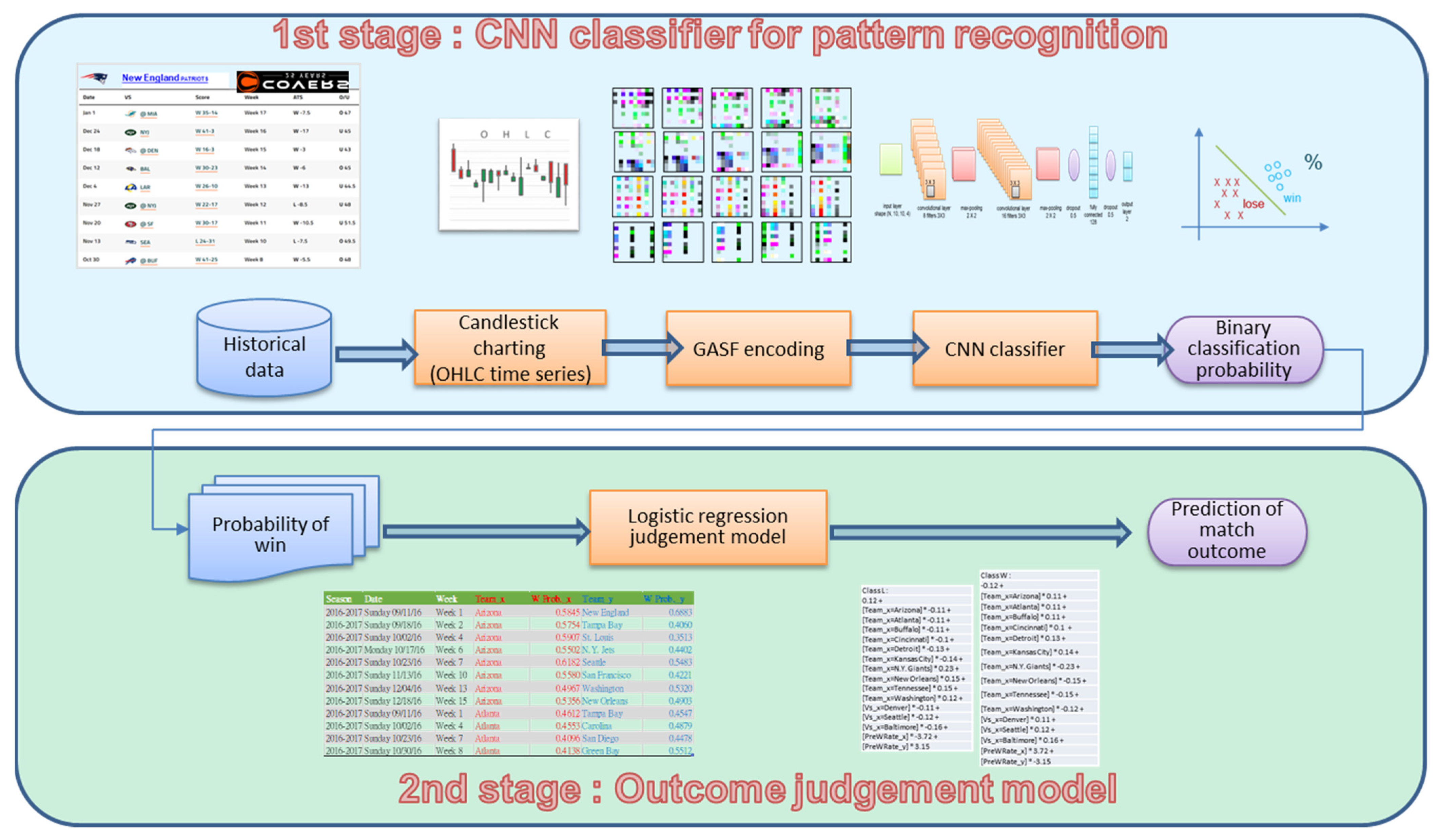
We propose a two-stage approach for the sports prediction model. The related framework is illustrated in
Figure 1.
In the first stage, we use CNN classifier to identify the behavior of each team. The win/loss fluctuations for each team are described by the time series data for each game in sequence. These data include the pre-game odds and actual points scored by each team in the game. These data are plotted as a candlestick to represent each game, and the consecutive candlesticks of several games represent the tendency of a team’s performance in sports matches. The candlestick representation of a sports competition is similar to a knowledge map that implies the behavioral patterns of victory and defeat. These candlesticks with unknown patterns are then imported into a CNN with powerful image recognition capabilities to classify winners and losers. To predict the results for the next match, the binary classification probability of win–loss is used.
In the second stage, we use the sports match outcome judgment model based on logistic regression. The predicted win probability of each team’s next outcome as obtained from the CNN in the previous stage will be used as the input for the judgment model. Given that the CNN win probabilities of both teams are estimated independently, the total win probability of these two teams is not equal to one. We need to use the judgment model to learn the CNN win probability and adjust the numerical difference of each team to determine the final result. For example, when a strong team with a 40% CNN win probability meets a weak team with an 80% CNN win probability, the result is not necessarily a loss for the strong team. Therefore, we introduce the historical matching pair and the associated CNN win probabilities into the judgment model to re-learn the behavior and determine the adjustment factors of each team, and to improve the accuracy of the outcome prediction.
3.2. Candlestick Representation of Sports Match Behavior
The candlestick representation of sports match behavior is taken from the odds of the betting market and the real score to generate an OHLC time series. Betting lines and their odds typically come in two types, one related to the difference in points scored by two teams and the other related to the total points scored by these teams. These spreads and total points scored are calculated after the game based on the actual points scored to decide whether a bet is won or lost. These spread, total points scored, and actual points scores are plotted for each team’s candlestick according to the method proposed by Mallios [
50]. Further details can be found in the article on sports metrics [
51] and the previous study [
20]. The candlestick chart defined by OHLC is formulated as follows:
where
D is the team winning/losing margin (i.e., the difference in points scored between the team and its opponent);
LD is the line (or spread) on the winning/losing margin between the team and its opponent (i.e., the side line in the betting market);
T is the total points scored by both teams;
LT is the line on the total points scored by both teams (i.e., the over/under (O/U) line in the betting market);
GSD presents the gambling shock related to the line on the winning/losing margin between the team and its opponent (i.e.,
D-
LD);
GST provides the gambling shock related to the line on the total points scored by both teams, which can calculate the difference between
LT (the line on the total points scored by both teams) and
T (the actual total points scored) (i.e.,
T-
LT).
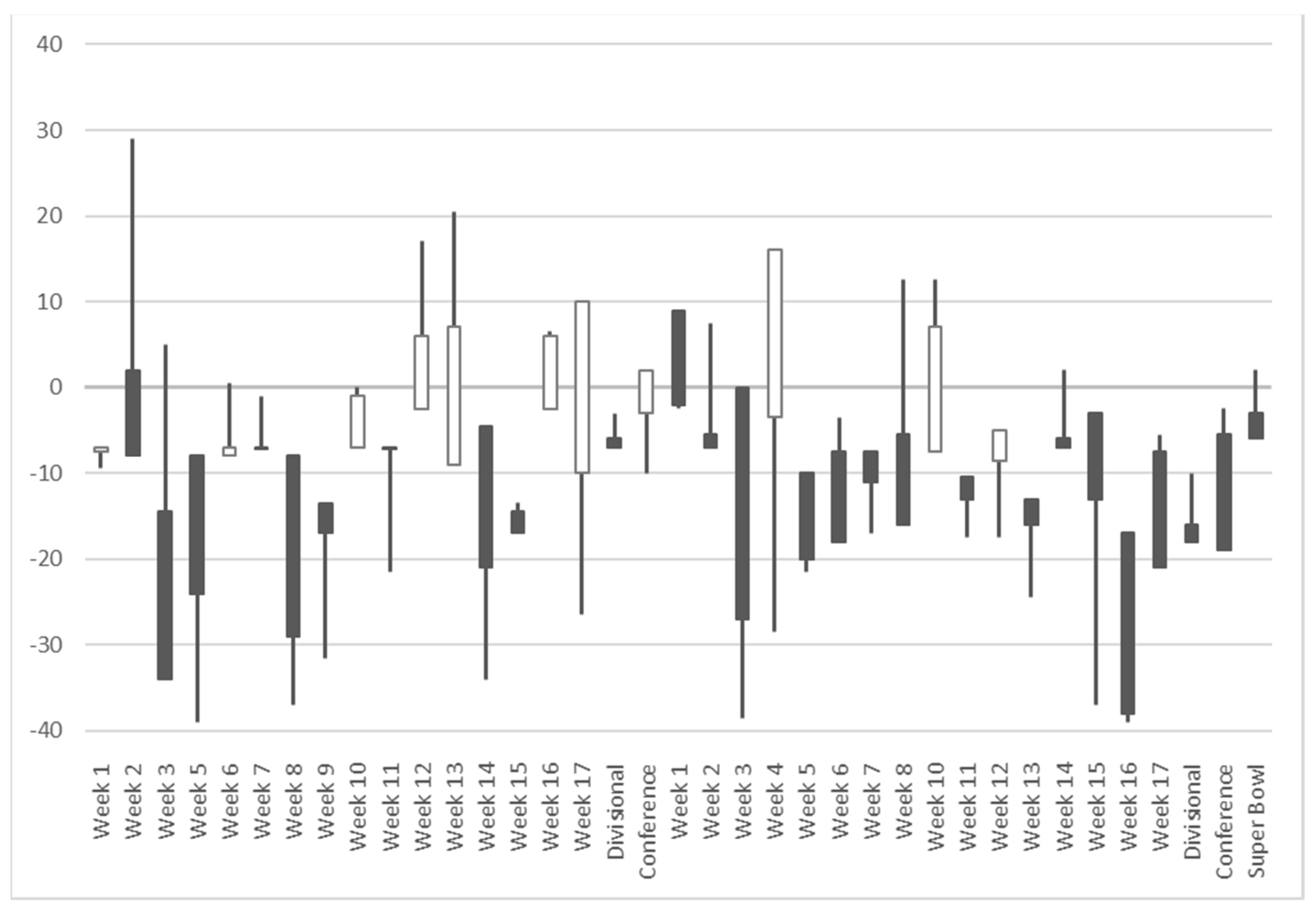
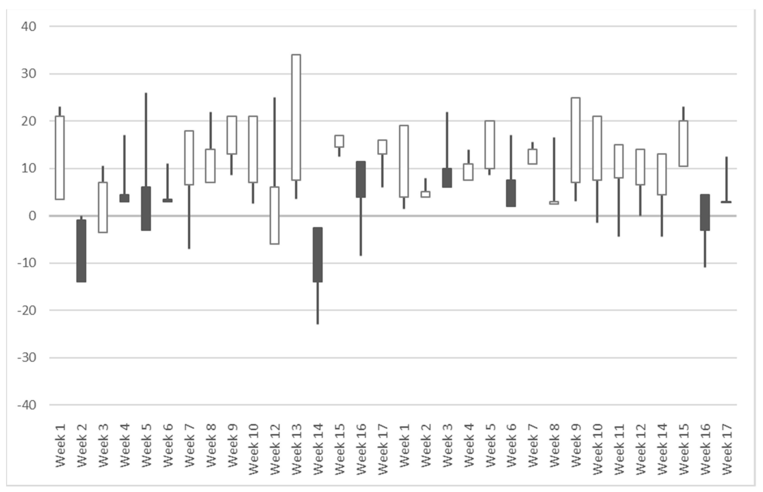
The candlestick chart for each team can be obtained in this manner. We take New England with the highest winning percentage and Cleveland with the lowest winning percentage of the 2017/2018 NFL season as examples, as shown in
Figure 2 and
Figure 3.
As shown in
Figure 2 and
Figure 3, the OHLC sports time series include positive and negative values, which greatly differ from the traditional time series of stock prices, where all values are greater than 0. The OHLC sports time series reflect the gap between two teams in the match. These time series are equivalent to the stationary return time series of the stock prices, which are derived by differencing its original non-stationary price time series. Stationary time series forms are beneficial for time series prediction modeling. However, the existence of meaningful patterns in sports candlesticks, such some identified patterns (e.g., morning star, bullish engulfing, etc.), warrants further investigation.
3.3. OHLC Time Series Data Encoding as Images by GAF
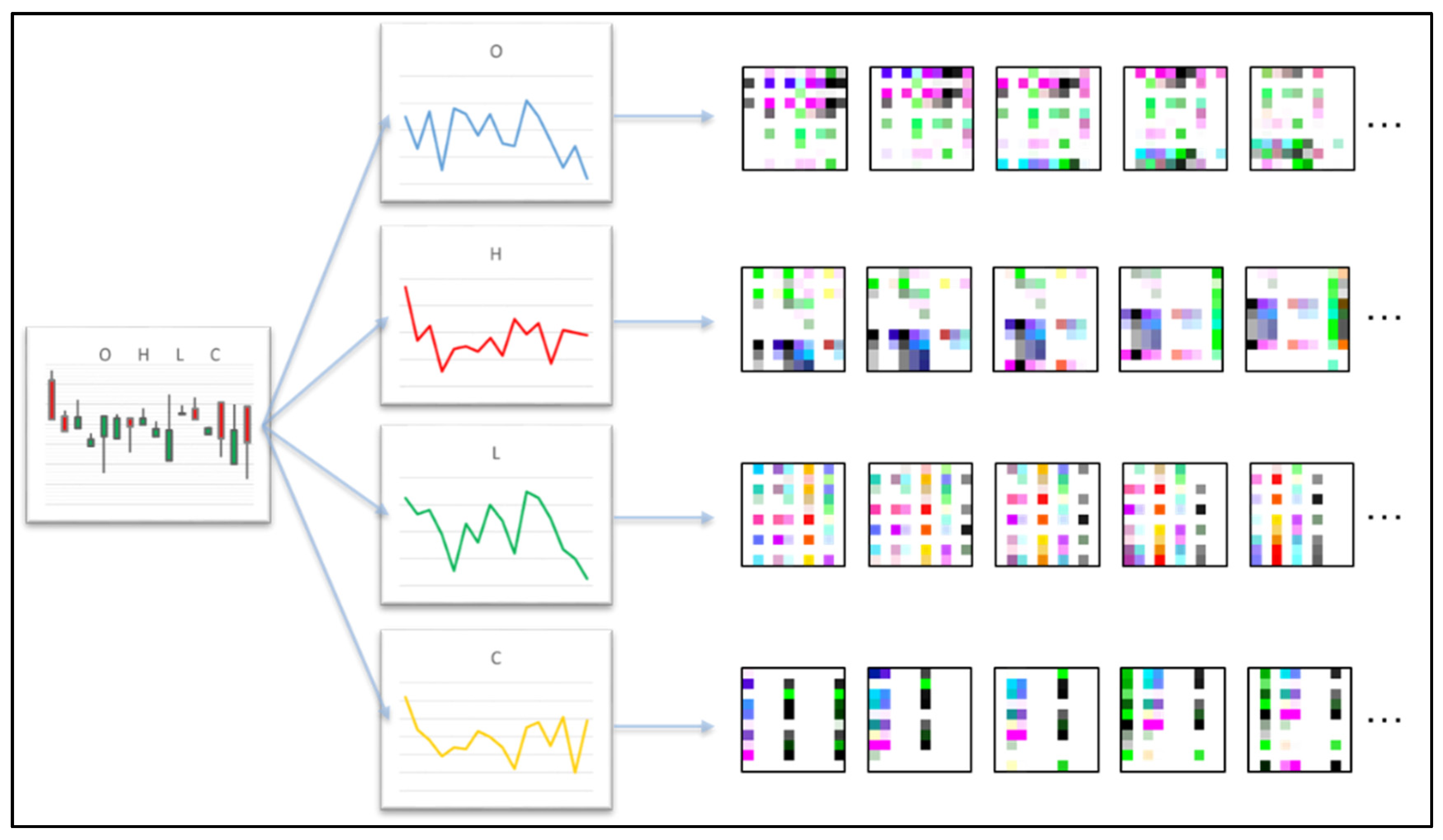
Although candlestick charts are examples of knowledge graphs, they cannot be directly fed into CNN because the appearance of candlesticks made of pixels will greatly vary depending on the scale of the drawing, the ratio of the x and y axes, and the size of the image pixels. Therefore, we use OHLC time series to represent candlesticks and address the inconsistency in candlestick appearance. The segmented 1D data of the original time series are converted into a 2D matrix, and the matrix size is treated as the pixel size of the graph. We use GAF to encode the time series as input images for computer vision.
First, time series
X = {
x1,
x2, …,
xn} is normalized to
by using Equation (6). Given that OHLC can either be negative or positive, the data are rescaled between –1 and 1.
The normalized data are then encoded into polar coordinates by calculating the angles and radius by using the angular cosine and time stamp. GASF uses the cosine function as defined in Equations (7) and (8). Each element of the GASF matrix represents the cosine of the summation of angles Ø. In the image matrix obtained by GASF, the diagonal elements from top-left to bottom-right represent the symmetric axis of the images, and the position corresponds to the original time series.
where
I is the unit row vector,
and
represent different row vectors.
We generate a 4D matrix that comprises the OHLC time series from the candlesticks. Each set of 1D time series data is encoded as 2D images by using GASF. Given that the candlestick representation includes all four OHLC time series, each series can be considered a channel that represents the image color. Given that we use the preceding 10 games to predict the next game, the input values of the CNN are 10×10 2D matrices in four channels as shown in
Figure 4.
3.4. Win Probability Estimation Based on CNN Classification
CNN specializes in image classification, and its accuracy has recently surpassed that of humans in various image recognition applications. With regard to the behavioral patterns in sports matches, we represent the odds and scores of matches as candlesticks in order to understand the fluctuations in time series. However, the time series transformed into 2D images by GAF is a highly in-depth knowledge graph, and humans cannot easily observe the features and patterns on this graph given their unknown style. Therefore, we exploit the classification capability of CNN to recognize the implied patterns from these image-based time series.
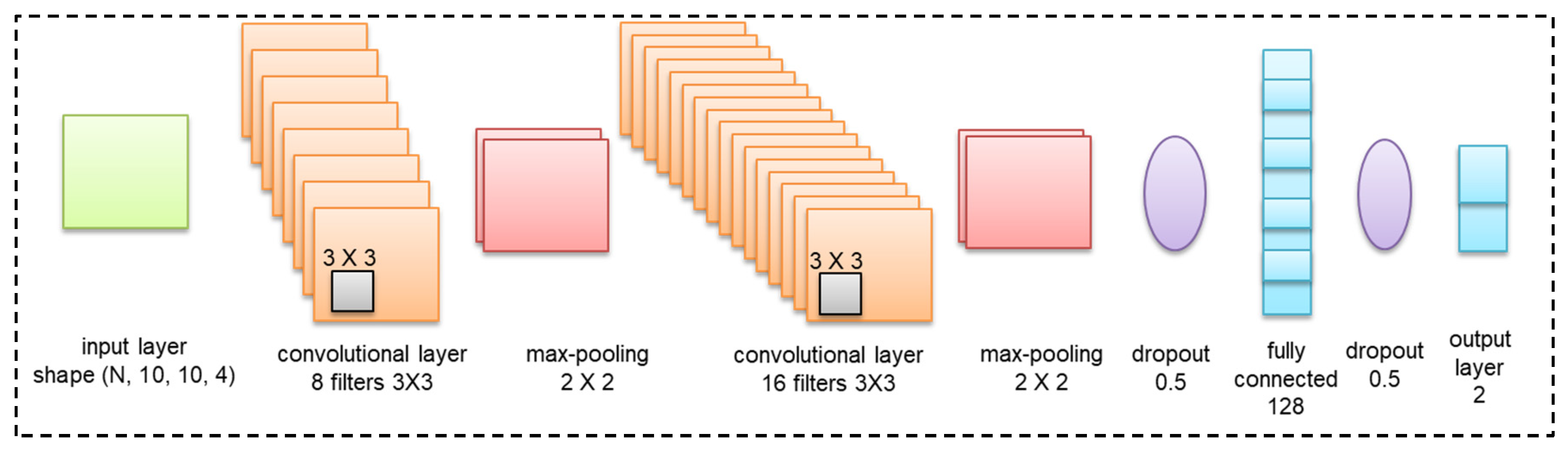
Figure 5 shows our CNN architecture, which originates from the most popular, small, and easy architecture, LeNet-5 [
56], and is enhanced by incorporating the concepts of rectified linear units (ReLU), max-pooling, and dropouts that have been proposed in recent years. After some testing and fine tuning, the adjusted architecture has been proven to work well.
As shown in
Figure 5, the CNN comprises two sets of convolutional, activation, and max-pooling layers followed by a dropout, fully connected layer, activation, another dropout, and a softmax classifier. The detailed structure and hyperparameters of each layer are described follows:
3.4.1. Input Layer
We encode the four OHLC time series that constitute the candlestick into 2D images with GADF as the input variable of CNN. We predict the next match outcome based on the information of the preceding 10 matches. We set the window size to 10 and fix the size of the 2D-transformed GADF image to a 10 × 10 pixel that comprises the four channels O, H, L, and C. After this step, the shape of the data matrices will be (10, 10, 4).
3.4.2. Convolution Layer
Two convolutional layers with a kernel size of 3 × 3 are used to match the input pixel size of 10 × 10, and the excitation function is set to the ReLU function.
3.4.3. Max-Pooling Layer
Two max-pooling layers with a window of 2 × 2 pixels are used for general image classification by calculating the maximum value for each patch of the feature map.
3.4.4. Dropout Layer
The data used for sports forecasting are expressed on a game-by-game basis. Despite having decades of retrospective data, our amount of data is far less than a million. Having a small amount of data can easily lead to overfitting problems when training CNN models. Therefore, we apply a dropout with a probability of 0.5 after the convolution and FC layers to reduce overfitting.
3.4.5. Fully Connected Layer
We apply two fully connected layers. The first layer is set with 128 dense and ReLU activation functions, and the second FC layer is set with the softmax activation function.
For our deep learning model, we select the adaptive learning optimizer Adam [
57] as our optimization algorithm to quickly obtain favorable results. To reduce the learning rate, which is typically necessary to achieve superior performance, we choose the simple learning rate schedule of reducing the learning rate by a constant factor when the performance metric plateaus on the validation/test set (commonly known as ReduceLRonPlateau). The output value of CNN represents the binary classification result of win or loss. We take the classification probability value of win for each team to determine the prediction outcome of the match by using the judgment model in the next stage.
3.5. Outcome Judgment Model of Logistic Regression
We use the CNN classifier to predict the next game based on the past performance of the team by using its own behavior as the learning object. This approach may be explained by the psychological changes in the morale and confidence of the team when facing an opponent and by the effect of the intensity of previous matches on the next match. However, given that the strong team has won many games in the past (thus making the CNN prediction to be mostly won), the CNN prediction for the weak team is mostly lost; this would make it very difficult to predict when a strong team meets another strong team or a weak team meets another weak team. Therefore, when the teams are separately classified as winners or losers in the first stage based on their historical behavior, we need to incorporate a judgment model that considers the win probabilities of both teams to determine the final predicted outcome.
Many studies that predict NFL game wins/losses have used a similar concept and dealt with numerical variables such as using the win probability [
58] of both teams as the output or calculating their rating scores and ranking [
59,
60,
61]. These teams are then compared before deciding the outcome. We take the probability values of the winning and losing classification results from the CNN classifier and feed them into the logistic regression model to learn and evaluate the final result.
The simple outcome judgment model is defined as follows. Considering team A vs. team B, the probability of each team winning the match is estimated by
Pa and
Pb. Given that
Pa and
Pb are estimated separately without considering the opponent, both of them take values between 0 and 1, and their total value ranges between 0 and 2 and is not necessarily equal to 1. If
Pa is greater than
Pb, then we predict that team A wins, and vice versa. The logistic regression judgment model takes the name of team A, the probability of winning
Pa, the name of opponent team B, and the probability of winning, a total of four variables, to build a prediction model, as shown in
Figure 6.
Logistic regression is a classification method that is especially suitable for predictive models with binary outcomes whose output values are restricted between 0 and 1 and can be interpreted as probabilities. Therefore, logistic regression has been used in predicting sports outcomes, such as soccer matches [
62], used together with a Markov chain model to predict National Collegiate Athletic Association football rankings [
63], or incorporated with data envelopment analysis to predict match outcomes of National Basketball Association [
64].
The outcome judgment model of the logistic regression is expressed as follows. Let Y be the variable of the binary reaction (win or loss) and p be the probability of win influenced by independent variable x. The relationship between p and x is given by:
The probability of success for event
Y is computed as:
When the strengths of both teams are close to each other, the difference between the classification probabilities originally obtained from the CNN is not significant. Such difference can be highlighted through an exponential change in the effect of the independent variables on the dependent ones in the logistic distribution to help determine the winner.
4. Experiments
4.1. Dataset
We collected 32 years’ worth of NFL match data from the 1985/1986 to 2016/2017 seasons to investigate CNN match outcome prediction models. These data include the odds of two betting lines and the actual points scored, which are publicly available and can be obtained from covers.com (
https://www.covers.com/sport/football/nfl/teams/main/buffalo-bills/2017-2018 (accessed on 29 October 2020) on a team-by-team, year-by-year basis via web crawling. The data were collected for both regular season and playoff games, covering a total of 18,944 games for 32 teams.
We organized our dataset by team and organized the time sequence of each team in the order of game time. The last game of the previous year was followed by the first game of the following year in the time series. The data for each team include various types of information (e.g., date, number of games, opponents, home or away games, win or loss results) and numerical data (e.g., point spread, line on side, line on total point, and points scored by both teams). These numerical data were converted into candlesticks to obtain four OHLC time series, and each 1D time series was converted into a 2D graph by GAF.
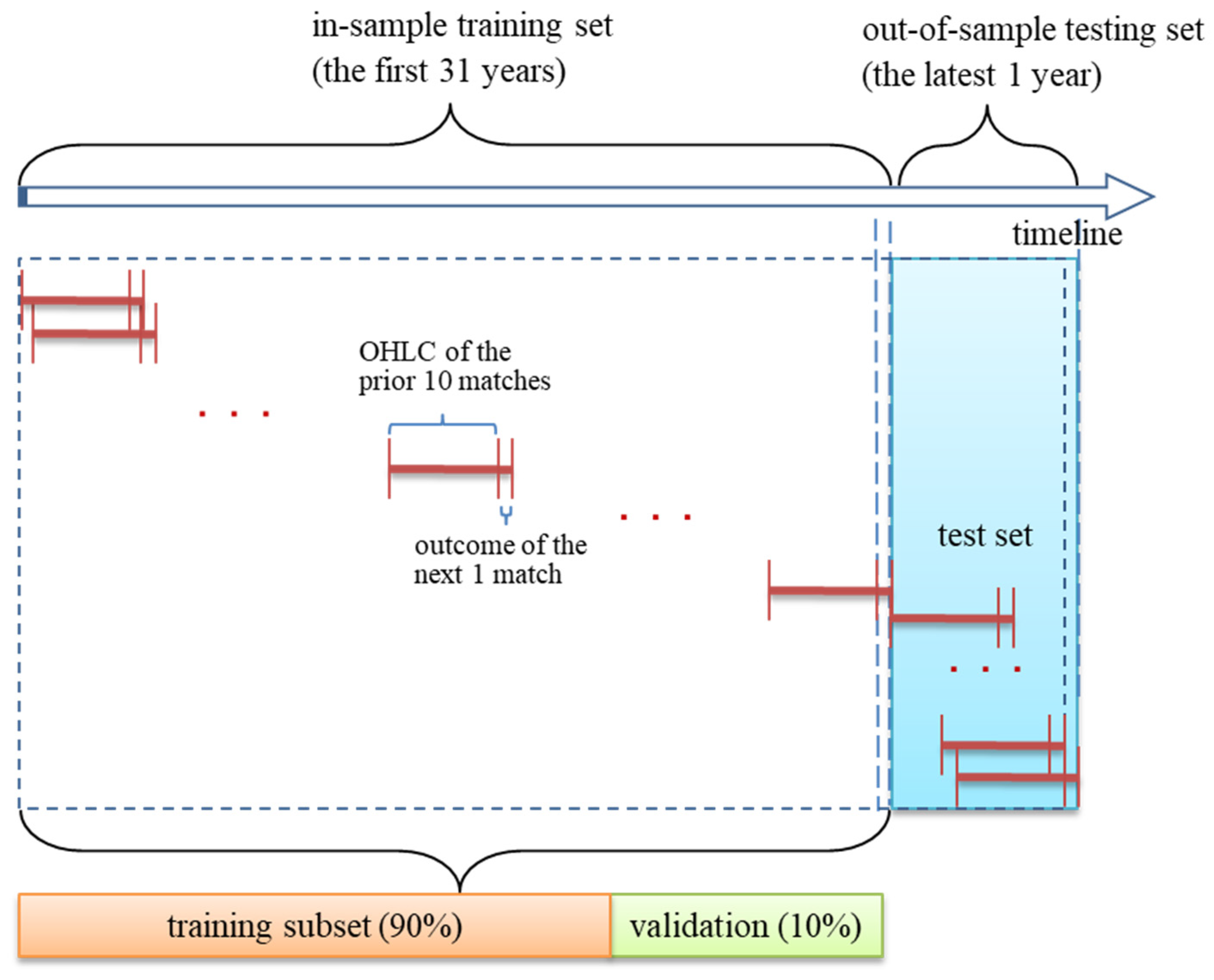
Figure 7 illustrates the data segmentation approach used to build a time series prediction model. First, we used the rolling windows approach by setting the window size to 10 (i.e., the candlestick of the previous 10 matches) and used CNN to find the implied behavioral patterns for predicting the next match. After windows rolling precession, we divided our dataset into the training and test sets by year. We used the first 31 years for the CNN model learning, and 90% and 10% of these data were randomly scattered as training and validation sets to verify the model learning. The last one was the test set, which serves as an out-of-sample assessment for ensuring the accuracy of predictions.
4.2. Experiment Designs
We conducted two series of experiments to verify the effectiveness and predictive performance of our proposed prediction model based on the sports candlestick pattern from all and individual teams and to test the approaches we used in the outcome judgment model. In the first experiment, we evaluated the effectiveness of GAF-encoded images derived from the OHLC series of sports candlesticks when classified by CNN in the first stage and tested whether the implied behavioral patterns for providing predictions should be based on the whole team or on individual teams. The second experiment aimed to test the performance of the two-team match outcome judgment model in the second stage. We used different machine learning algorithms to check whether the prediction performance was acceptable when compared with each other and with the comparison group.
To evaluate the experiment results, for the first stage of CNN classification capability, we compared the accuracy of the test sets. For the second stage, we assessed the performance of the outcome prediction models based on different machine learning approaches, which in turn were assessed based on the accuracy of the win/lose outcome. The precision, recall, and F-measure corresponding to the outcome were also computed to reveal further details. A higher value of these measures is generally favored. These measures are defined as follows:
where
TP,
TN,
FP, and
FN refer to true positive, true negative, false positive, and false negative, respectively.
To further compare whether the two-stage approach proposed in this study helps to improve the single-stage approach, we also build a logistic regression model for OHLC time series in the first stage. We normalize the OHLC time series using Equation (6) and set the window size to 10, making it consistent with the input values used for the GAF conversion in the first stage CNN classifier. Therefore, the input values of the logistic regression model in the first stage are the team name, the opponent team name, the team’s OHLC value in the preceding 10 consecutive games, and the opponent team’s OHLC value in the preceding 10 consecutive games, a total of 82 variables. The output value is the team’s win or loss in the present match.
The experimental results were also compared with “betting” and “home” as benchmarks. Betting refers to the bookmaker’s prediction, which is based on the betting odds of the winning/losing margin. A negative value indicates a win, whereas a positive value indicates a loss. Home refers to the well-known home field advantage, where the home team is always predicted to win.
The kappa coefficient is a measure of inter-rater agreement involving binary forecasts, such as win–lose [
65]. We used this coefficient to measure the levels of agreement among the proposed prediction model, the comparison groups, and the actual outcome.
4.3. Comparison of Candlestick Pattern Recognition with CNN
Our first task was to examine whether the patterns implied by sports candlesticks can reflect past behavior and if they are useful in predictive models. Several patterns in stock market candlesticks have been proven to be useful in explaining investor behavior and forecasting purposes. These patterns are not limited to a particular stock but can be applied to any stock. Therefore, we checked for common behavioral patterns among different teams based on sports candlesticks. We conducted two experiments by using the data of all teams and the data of each team as our data source for CNN learning. The experiment results reveal that either all teams share a common pattern or that each team is suitable for the prediction based on their historical behavioral patterns. The results are shown in
Table 1.
Table 1 lists the teams in a descending order according to their actual win percentage; that is, the percentage of wins out of all matches played during the test period. The prediction accuracy of the two experiments was grouped into three measures: the CNN prediction classification in the first stage, the simple judgment in the second stage, and the logistic regression judgment models in the second stage.
First, we investigated the utility of our two-stage approach by comparing the CNN classifier prediction results in the first stage with the judgment model results in the second stage. Based on the average accuracy obtained in all prediction cases, we found in both experiments that the accuracy is lowest if only the first-stage CNN was used. However, such accuracy improves when the second-stage judgment model was added. This model considers the CNN prediction values of both teams in the match. Only slight improvements in accuracy were observed when the simple judgment model was used, and the best accuracy was obtained when using logistic regression.
Second, we compared the effect of introducing overall and individual behaviors into the prediction model. The prediction accuracy of using overall behavior was less acceptable than that of using individual behavior, and the average accuracy of the best logistic regression judgment model was only 60.30%, which was not meaningful. Meanwhile, the average accuracy of using individual behavior, whether CNN, simple judgment, or logistic regression judgment, was high, with the best logistic regression judgment model reaching an acceptable value of 69.29%.
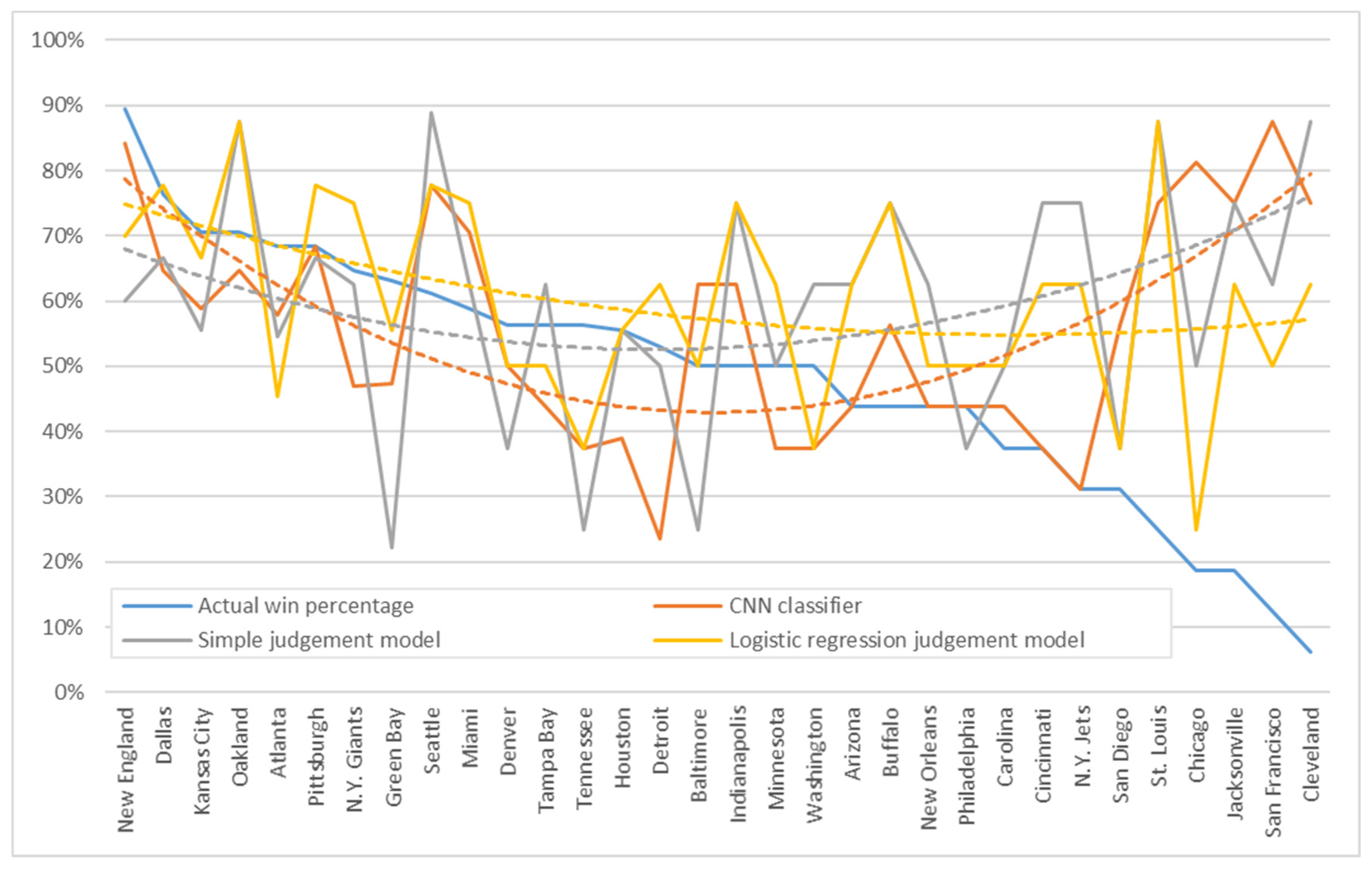
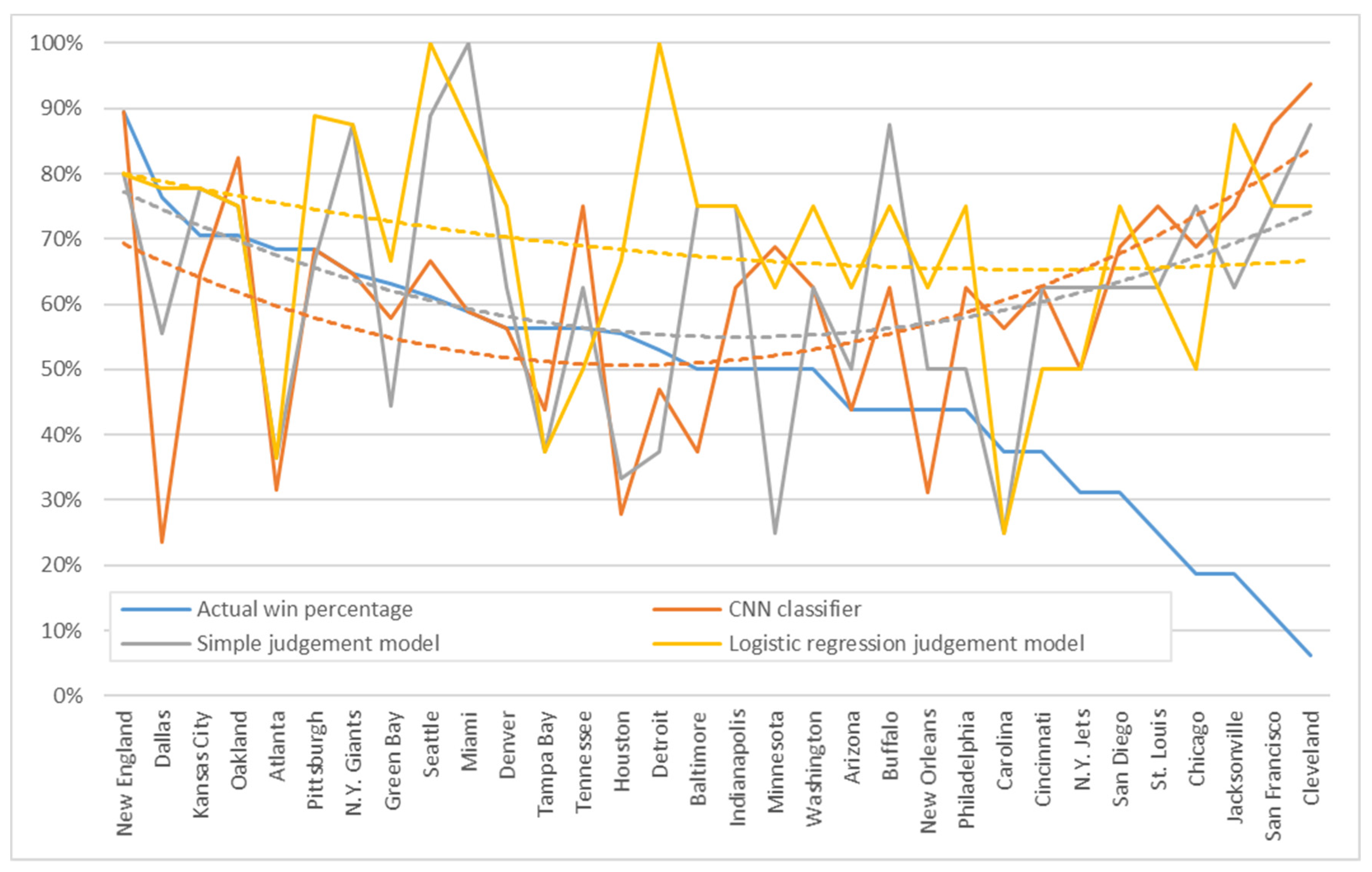
Third, we addressed the differences across each team in the prediction models. We plotted the accuracies of the CNN prediction classification and judgment model according to the overall and individual behaviors in
Figure 7 and
Figure 8, respectively. The x-axis denotes the ranking of actual win percentage, which represents the strength of the team, and an x-value of 1 is ranked first. Meanwhile, the y-axis shows the accuracy with values ranging from 0% to 100%. The curves of accuracy were added to the figure with trend lines to highlight the tendency of each team’s strength and weakness rankings.
Figure 8 presents the results of the overall behavior experiment. The teams on the left and right sides of the graph reported higher accuracies than those at the center. The trend line showed a smile-like curve, thereby suggesting that the strong and weak teams had fixed behaviors in terms of winning and losing, thereby facilitating predictions.
Figure 9 presents the results of the individual behavior experiment. The prediction accuracy of the team at the center of the graph improved compared to that shown in
Figure 8. Although such accuracy varied across teams, the trend line was close to the same level, thereby indicating the minimal difference between the strong and weak teams.
4.4. Comparison of Different Approaches in the Outcome Judgment Model
We used the best learning strategy for each team to learn individually based on their own data. After building the CNN classifier in the first stage, we calculated the CNN prediction values of all experimental data, including those for the training and test set. In the second stage of the judgment model, we used the CNN output values of both teams in the training set to learn the judgment model and then verified the final prediction performance in the test period.
In addition to logistic regression and the simple judgment model, we adopted sequential minimal optimization (SMO) for support vector machines (SVM), Naïve Bayes, Adaboost, J48, random forests, and multi-objective evolutionary algorithms (MOEA) for fuzzy classification, which are commonly used in machine learning, in our experiments to compare the prediction accuracy of the judgment model. The results are shown in
Table 2.
Table 2 also presents the accuracy of two single-stage models, and these values were used as benchmarks for comparison with two-stage models. As shown in
Table 2, the accuracies of the first-stage CNN classification and the first-stage logistic regression were 60.11% and 61.42%, respectively. It revealed that when using OHLC time series to build a prediction model for sports matches, the CNN classifier with graphical classification to process the time series was not as accurate as the logistic regression model that took into account the strengths and weaknesses of the two teams. Although these values of the single-stage model were higher than the 58.05% accuracy of home in the comparison group, they were not as good as the 63.67% accuracy of betting.
After incorporating the second stage to the output values of the first stage CNN classifier, the accuracy of random forest decreased, whereas that of Naïve Bayes grew slightly larger than that of simple judgment. The rest of the machine learning algorithms increased the prediction accuracy above that of betting (63.67%), and the best-performing logistic regression judgment model reported an accuracy of 69.29%.
Table 2 also lists the kappa coefficients for comparing the level of agreement with the actual outcome and facilitating a fine-grained comparison. The kappa coefficients of all approaches were below 0.4, with only the logistic regression and Adaboost obtaining coefficients above 0.3.
We conducted McNemar tests to examine whether the logistic regression model in the second stage significantly improved the first-stage results and outperformed the betting model. This nonparametric test is designed for two related samples and is particularly useful for the before-and-after measurements of the same subjects [
66].
Table 3 presents the results. As shown in the table, the logistic regression judgment model significantly differed from the simple judgment model and the first-stage CNN classifier in that both of them rejected the null hypothesis. This proved that by adding the logistic regression judgment model in the second stage, it is significantly different from the one-stage only CNN prediction model. With the help of judgment in the second stage, the improvement of prediction accuracy is significant. The McNemar value between the logistic regression judgment model and the betting market prediction was 0.468, whereas the p value was 0.494, thereby supporting the null hypothesis that the performances of both models are the same. The logistic regression judgment model outperformed the betting market prediction but did not reach the 0.05 statistical significance level.
4.5. Discussion
By using CNN to learn the data of all teams, the binary prediction performance was not satisfactory when used to predict the classification of each team in the next match. The second stage of the judgment model, which simultaneously considers both teams in the match, is necessary to improve accuracy. Each team should learn individually with their own data and build their own CNN classifier. A total of 32 CNN classifiers were associated with 32 teams instead of using all data to construct a common CNN classifier. This approach is in line with the concept of some prediction methods in sports, where teams are initially grouped according to their performance and specific models are built for each group [
67].
In the second stage, the logistic regression model is significantly more effective than the other machine learning methods probably due to the fact that when only the names and CNN prediction values of the two teams (total of four variables) are used to predict the victory or defeat of the home team, the logistic regression can simply yield different weights and either add or subtract points to adjust the prediction value for each team from the historical data. Other methods may require additional data, such as past performance indicators, and additional variables in the composition of players to be equally effective.
The two-stage approach proposed in this study, incorporating the CNN classifier in the first stage and the logistic regression in the second stage, would yield several benefits. The combination of the two results in a considerable improvement in prediction accuracy over the CNN classifier and logistic regression alone and outperforms the betting market prediction. Another benefit is that the use of match scores and betting odds as raw data is a universal approach to predicting without restrictions on the type of sport. There is no need to think about which performance metrics, such as earned run average and batting average in baseball, or real plus–minus and pace in basketball, to use as features in the model. In contrast to recent two studies on machine learning for NFL game outcome prediction, Hsu [
20] similarly used features derived from candlestick charts based on betting odds and scores as input variables to makes one-step ahead predictions. These features include the difference and the proportion of change between the preceding and following match data. A total of 19 and 28 features were selected as the input variables for the classification-based model and the regression-based model, respectively. Both models were examined using five different methods of machine learning. Another study by Beal et al. [
68] tested the nine different machine learning classification techniques using a total of 42 features for each team. These 42 features were derived from scores and performance metrics, using the current season average up to that game and the average across the most recent completed season. The total number of features of the two teams in a match was 84, and with considering the home advantage, a total of 85 parameters were used as input values for the prediction model. Although both studies are able to outperform the bookmaker’s prediction accuracy, they are accompanied by a number of features that need to be considered as input variables in the prediction model.
However, such time series-based models that we adopt are inevitably challenged as overly simplistic and difficult to represent sports matches. Complementarily, the complicated deep learning algorithms processed in the CNN are used to learn the features of different sports matches and different teams within the time series. The drawbacks of this approach come from the CNN. The network topology and hyperparameter settings of CNNs are not easy to determine with a trial-and-error approach. Moreover, such machine learning methods are more computationally intensive than traditional statistically based methods.
5. Conclusions
CNN and deep learning have made great achievements in the fields of computer vision and natural language processing. However, limited progress has been made in sports analysis and prediction, which mostly rely on visual materials, such as videos of competitions or player position maps. CNN shows difficulties in exploiting its capabilities for 1D data types. Therefore, a predictive model cannot be directly constructed with CNN for sports matches, which are often considered discrete and independent.
To take advantage of the achievements of CNN in computer vision, we proposed a two-stage approach for predicting sports match outcomes. The raw data of the odds and points scored in the betting market were processed through a series of transformations into candlestick expressions comprising time series. Afterward, we used GAF to encode the time series into 2D images in order for them to converge with the CNN of the first stage. The second stage of the judgment model based on logistic regression was then incorporated to consolidate the CNN output for prediction.
Our experimental comparisons reveal that for predicting wins and losses, the historical data imply some associations and behavioral patterns between pre- and post-games that can be used for the prediction. The behavioral patterns implied by individual teams are more useful for the prediction than the behavioral patterns implied by all teams. In addition, predicting the match outcome directly with the CNN of the first stage is not ideal. However, the prediction performance of the CNN was improved significantly by the proposed two-stage approach with the logistic regression judgment model and achieves a prediction accuracy of 69%, which was superior to the betting market.
Future studies are suggested to further investigate the feasibility of using the proposed two-stage model in other sports matches. The hyperparameter tuning problem, which is often encountered when using CNN, can be further tested to improve prediction accuracy. Future research could be directed towards identifying opportunities for incorporating emerging deep learning techniques from traditional sports prediction methods, such as performance metrics and ranking/rating systems, and modifying them to achieve cutting-edge prediction models that keep pace with computational intelligence technology.


