
Reverse Logistics Location Based on Energy Consumption: Modeling and Multi-Objective Optimization Method


Abstract
1. Introduction
2. Reverse Logistics Facility Location Model
2.1. Problem Description
2.1.1. Assumptions
2.1.2. Model Parameters
- Logistics facility
- Classification of waste products
- Cost of recycling
- Decision variable
2.2. Target Function of Considering Carbon Emission
2.2.1. Carbon Emission Cost Calculation
2.2.2. Establishment of Dual Objective Functions
- Constraints
3. Solution Methodology
3.1. Gravity Algorithm
3.2. The Gravitational Particle Swarm Optimization Algorithm
3.3. The Framework of the Proposed Multi-Objective Algorithm
- Coding mode
- Generate the initial particle swarm
| Algorithm 1. Initial Particle Swarm Generation |
| Input: NIND (Particle swarm size), N (The number of urban points) Output: Pop (Initial population) |
| (1) i = 1; (2) While i < = NIND Do (3) Pop (i) = zeros (n*2); (4) M = unidrnd (N) (5) While M < Pmin or M > Pmax Do (6) M = unidrnd (N); (7) N = unidrnd (N) (8) While N < Dmin or N > Dmax Do (9) N = unidrnd (N); (10) Use above gotten M and N. Choose randomly the city waiting for site selection. And the corresponding location code of the individual is changed to 1. (11) i++; (12) End While. |
- Adaptive value calculation and Pareto solution screening
| Algorithm 2. Pareto Rank and Crowding Distance Calculation of Particle Swarm Individuals |
| Input: Pop (swarm) Output: P (record Pareto rank of the particle swarm); S (record particle crowding distance of the particle swarm) |
| (1) Use the target formula to calculate the target value of particle swarm individuals. The transportation of waste products among logistics facilities is based on the principle of the nearest point. Only when the destination facility reaches its maximum capacity can they proceed to the next nearest point. The target value also needs to be transformed through fitness, and two targets value are transformed the fitness value with the smaller the better. (2) i = 1 (3) While i < = NIND Do (4) Initialize P(i) = 0; (5) For Pop(i), traversal the whole particle swarm. If there is a particle j and a relationship between its fitness value and fitness value of individual i: f1(i) > f1(j) and f2(i) > f2(j), Do (6) P(i)++; (7) For particle i, use the Euclidean distance between particles to calculate its crowding degree S(i); (8) End While. |
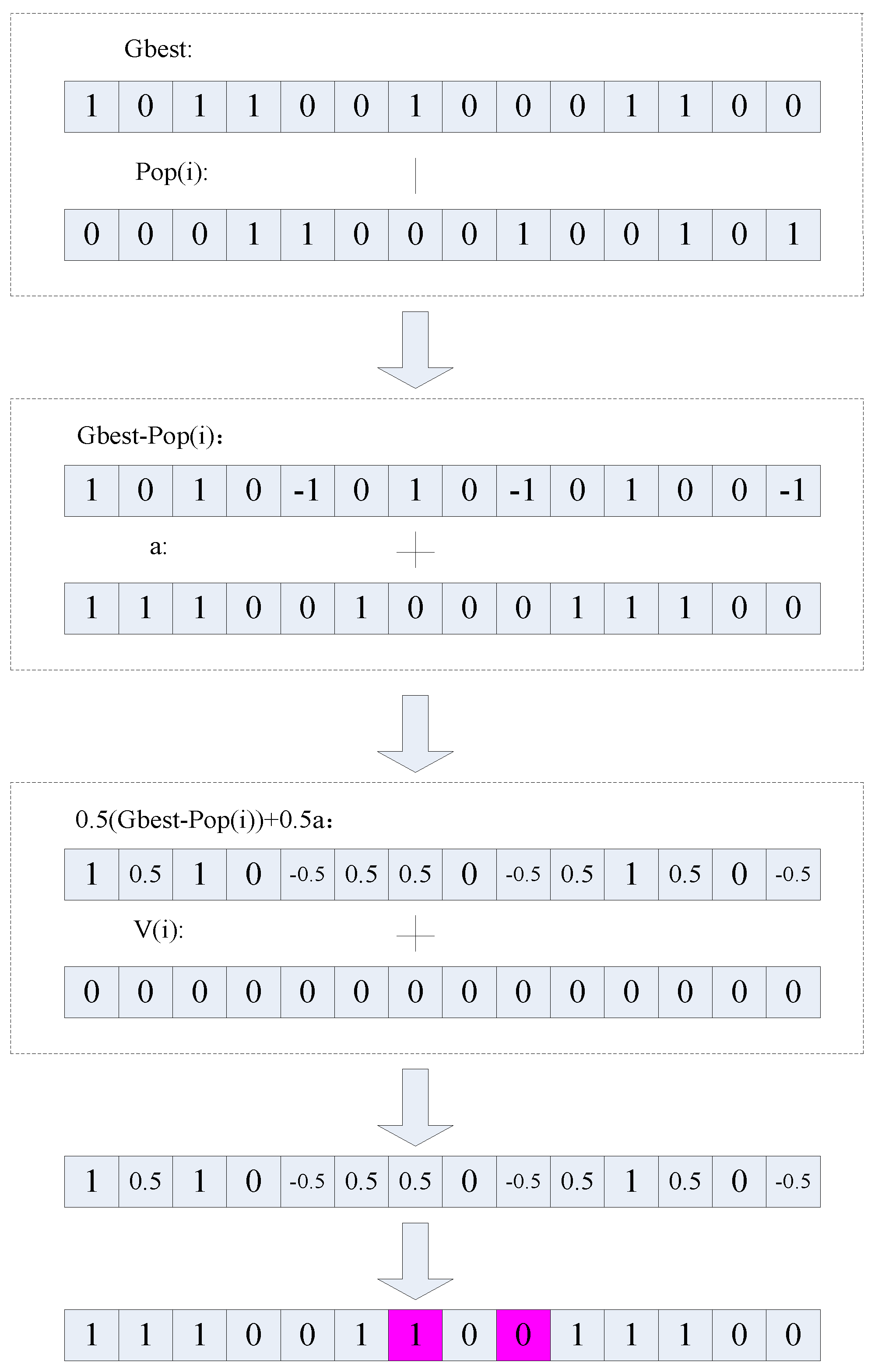
- Individual update
| Algorithm 3. Individual Update |
| Input: Pop, P, S Output: PopNew (New particle swarm) |
| (1) i = 1 (2) While i < = NIND Do (3) Initialize the particle velocity Vi = 0; (4) Calculate the particle accelerated velocity of individual i through the formula for calculating the acceleration of gravity. (5) The superior individuals in the dominant solution set were randomly selected as GBest. (6) Calculate the velocity Vi of the particle i. (7) Obtain the new solution of particle i. (8) i++; (9) End While. |
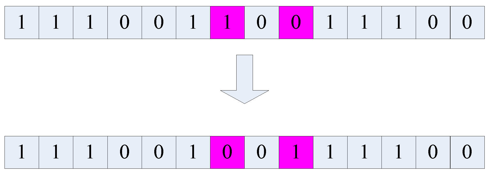
| Algorithm 4. Feasibility of Correction Solution |
| Input: Pop(i) Output: PopNew(i) |
| (1) M = Find(Pop(i, 1: N) == 1) (2) If M < Pmin or M > Pmax Do (3) If M > Pmax, the city point of after reaching the upper limit of the number of classification points is changed to 0; If M < Pmin, the non-1 city point is randomly selected and changed to 1 until M satisfies the constraint. (4) M = Find (Pop(i, N + 1: N + N) == 1) (5) If M < Dmin or M > Dmax Do (6) If M > Dmax, the city point of after reaching the upper limit of the number of classification points is changed to 0; If M < Dmin, the non-1 city point is randomly selected and changed to 1 until M satisfies the constraint. (7) End. |
- Update swarm
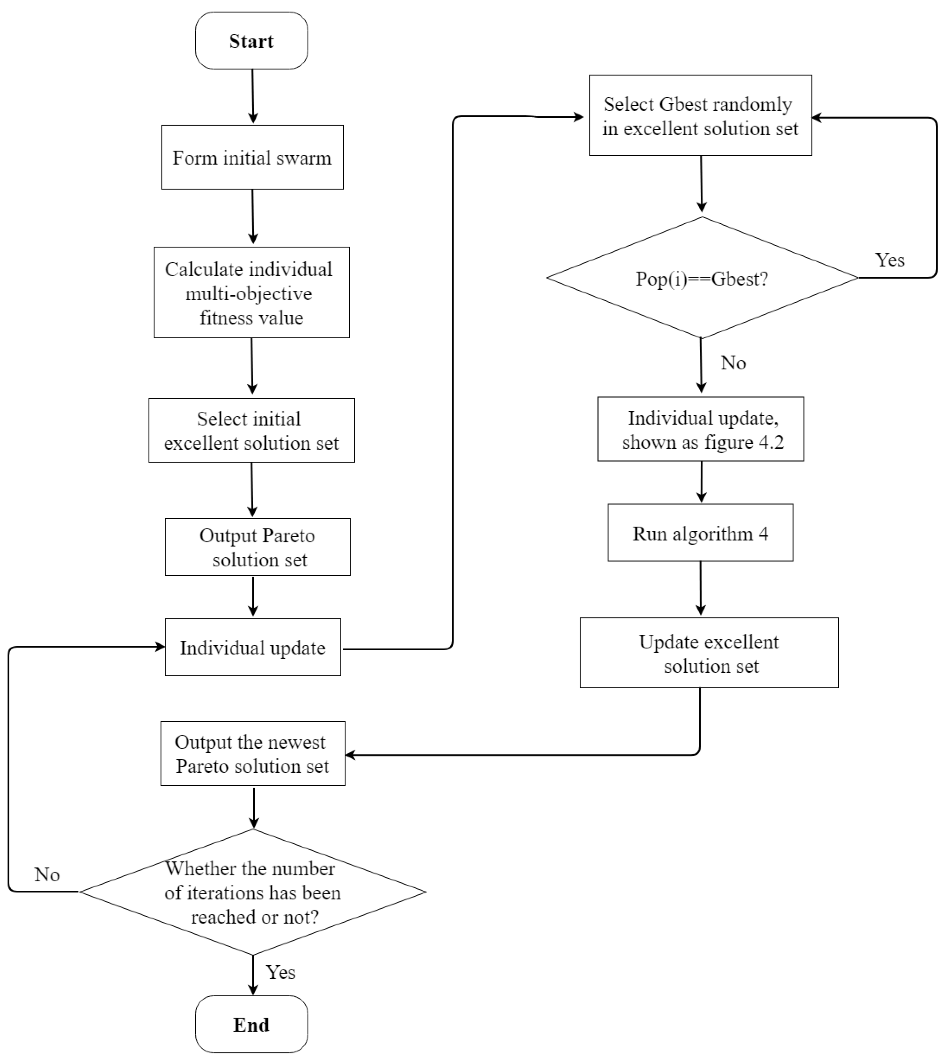
- Improve Gravity multi-objective algorithm flow
4. Case Study
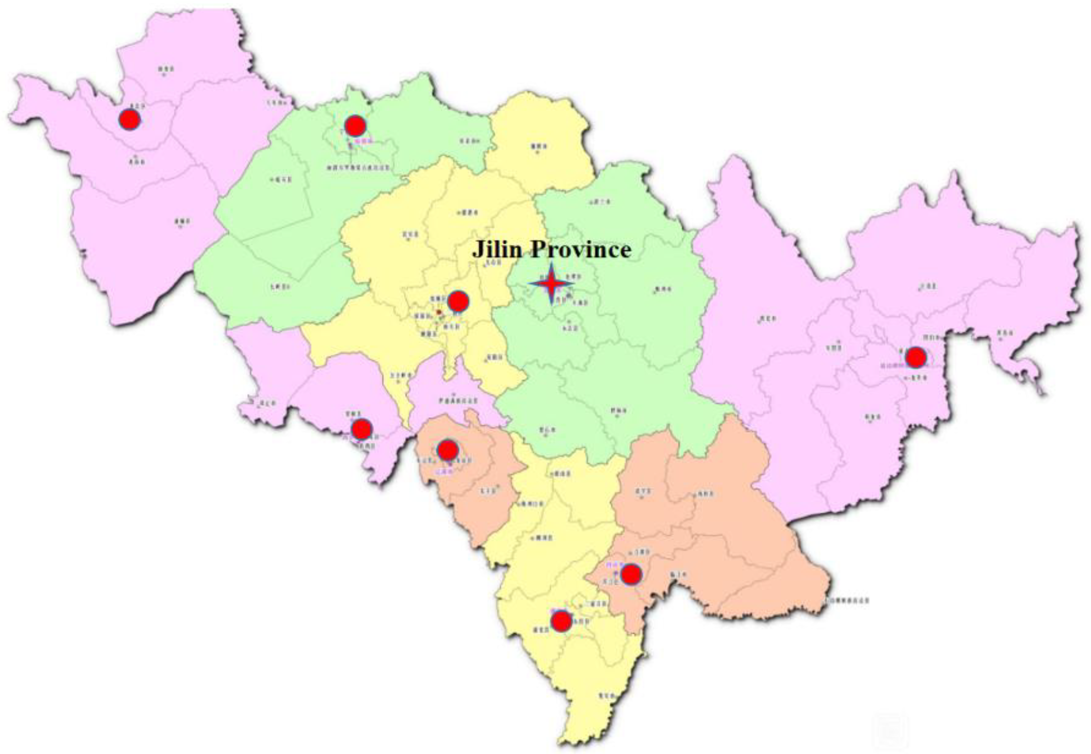
4.1. Background
4.1.1. Description of Basic Situation
4.1.2. Analysis of Mobile Phone Recycling Value
4.1.3. Analysis of Mobile Phone Recovery Cost
4.2. Results and Analysis
4.2.1. Optimization Results
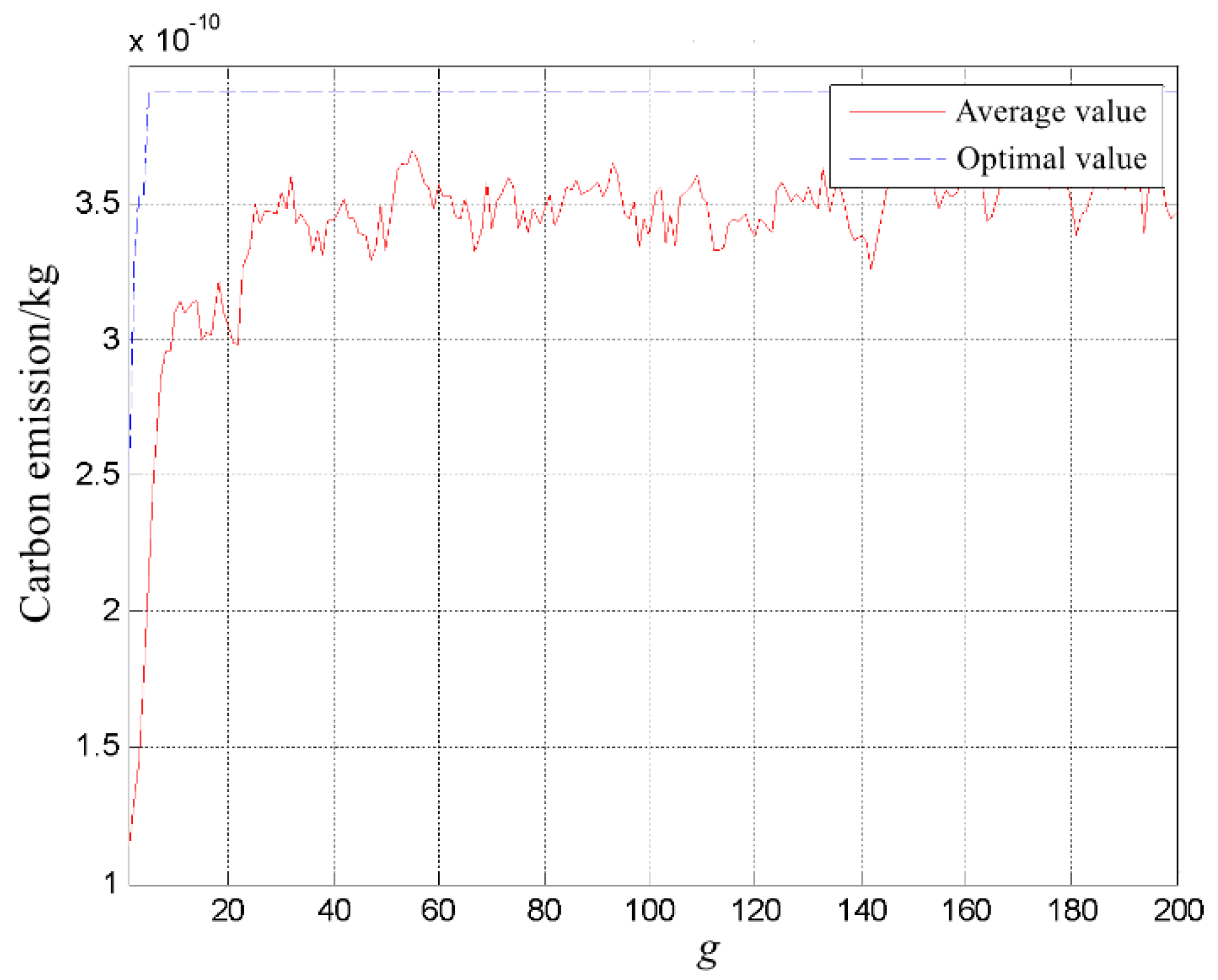
- Consider only the case where carbon emissions are minimal
| 1 | 1 | 1 | 0 | 1 | 0 | 0 | 0 | 1 | 1 | 1 | 1 | 0 | 0 | 0 | 0 | 1 | 0 |
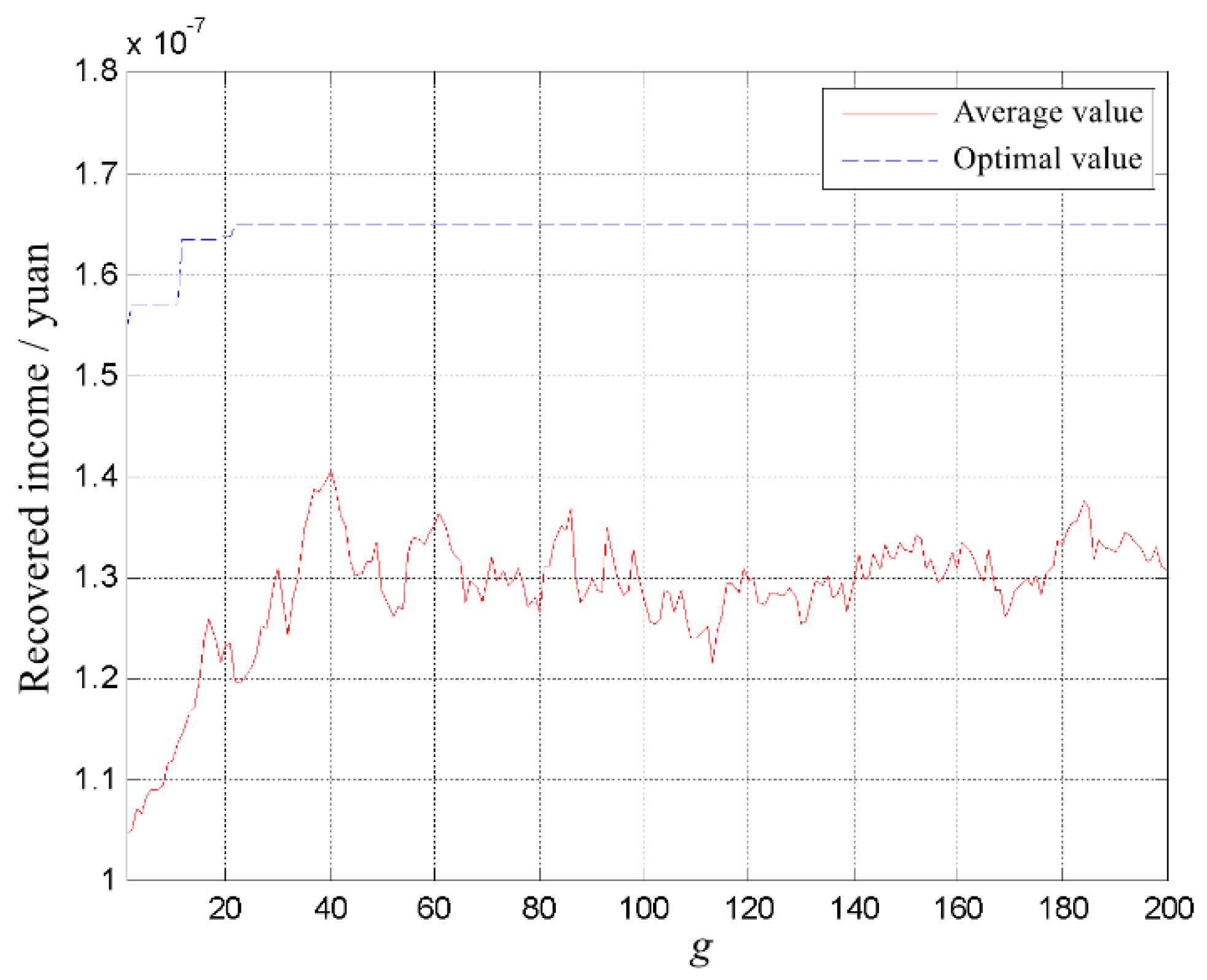
- Consider only the case of maximum benefit
| 1 | 1 | 0 | 1 | 0 | 0 | 1 | 0 | 0 | 0 | 1 | 1 | 0 | 0 | 0 | 0 | 0 | 0 |
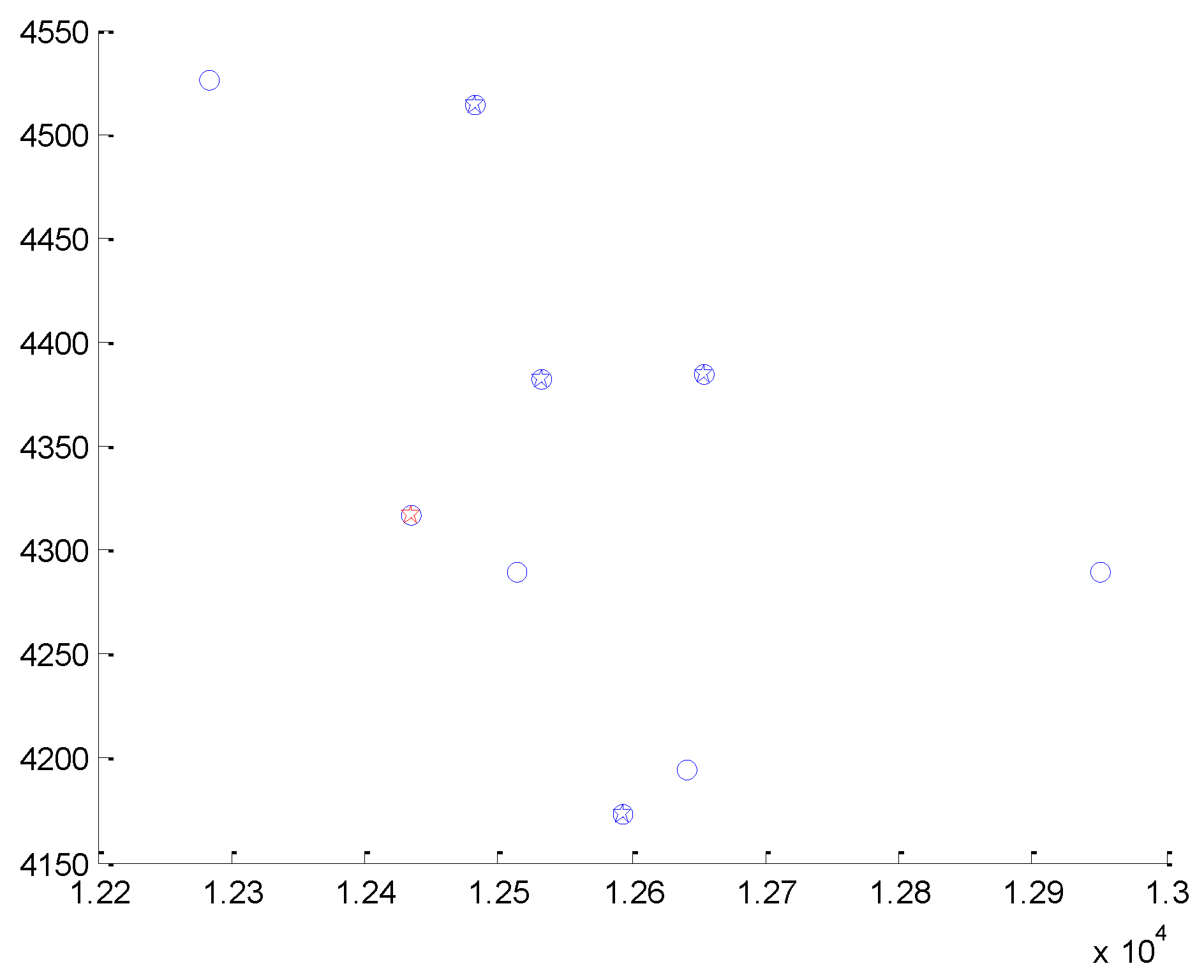
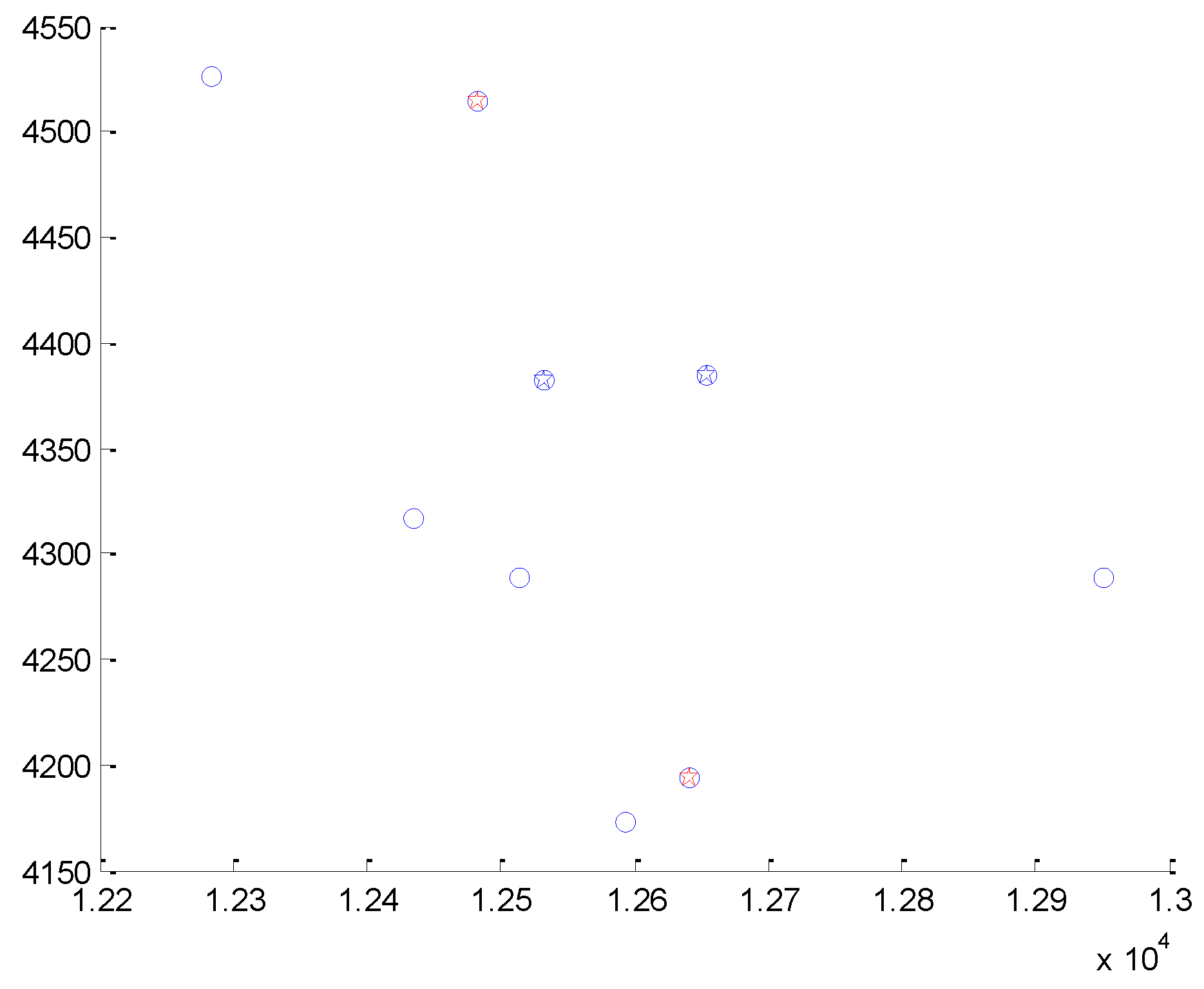
- Consider dual targets of carbon emissions and recycling revenue
4.2.2. Sensitivity Analysis
4.2.3. Discussion
5. Conclusions
Author Contributions
Funding
Institutional Review Board Statement
Informed Consent Statement
Conflicts of Interest
References
- Lv, J.; Du, S. Kriging Method-Based Return Prediction of Waste Electrical and Electronic Equipment in Reverse Logistics. Appl. Sci. 2021, 11, 3536. [Google Scholar] [CrossRef]
- Zhou, X.H.; Cheng, S.J.; Cheng, P.F. Multi cycle and multi objective location planning for remanufacturing reverse logistics network under self recycling mode. Syst. Eng. 2018, 36, 146–153. [Google Scholar]
- Lee, C.; Chan, T. Development of RFID-based Reverse Logistics System. Expert Syst. Appl. 2009, 36, 9299–9307. [Google Scholar] [CrossRef]
- Zhang, C.; Fathollahi-Fard, A.; Li, J.; Tian, G.; Zhang, T. Disassembly Sequence Planning for Intelligent Manufacturing Using Social Engineering Optimizer. Symmetry 2021, 13, 663. [Google Scholar] [CrossRef]
- Sung, S.-I.; Kim, Y.-S.; Kim, H.-S. Study on Reverse Logistics Focused on Developing the Collection Signal Algorithm Based on the Sensor Data and the Concept of Industry 4.0. Appl. Sci. 2020, 10, 5016. [Google Scholar] [CrossRef]
- Huscroft, J.R.; Hazen, B.T.; Hall, D.J.; Hanna, J.B. Task-technology fit for reverse logistics performance. Int. J. Logist. Manag. 2013, 24, 230–246. [Google Scholar] [CrossRef]
- Savaskan, R.C.; Bhattacharya, S.; Van Wassenhove, L.N. Closed-Loop Supply Chain Models with Product Remanufacturing. Manag. Sci. 2004, 50, 239–252. [Google Scholar] [CrossRef]
- Park, S.Y.; Keh, H.T. Modelling hybrid distribution channels: A game-theoretic analysis. J. Retail. Consum. Serv. 2003, 10, 155–167. [Google Scholar] [CrossRef]
- Liu, H.; Lei, M.; Deng, H.; Leong, G.K.; Huang, T. A dual channel, quality-based price competition model for the WEEE recycling market with government subsidy. Omega 2016, 59, 290–302. [Google Scholar] [CrossRef]
- Islam, M.T.; Huda, N. Assessing the recycling potential of “unregulated” e-waste in Australia. Resour. Conserv. Recycl. 2020, 152, 104526. [Google Scholar] [CrossRef]
- Shih, L.-H. Reverse logistics system planning for recycling electrical appliances and computers in Taiwan. Resour. Conserv. Recycl. 2001, 32, 55–72. [Google Scholar] [CrossRef]
- Lee, D.-H.; Dong, M.; Bian, W. The design of sustainable logistics network under uncertainty. Int. J. Prod. Econ. 2010, 128, 159–166. [Google Scholar] [CrossRef]
- Johnson, F.; Vega, J.; Cabrera, G.; Cabrera, E. Ant Colony System for a Problem in Reverse Logistic. Stud. Inform. Control 2015, 24, 133–140. [Google Scholar] [CrossRef]
- Pishvaee, M.S.; Kianfar, K.; Karimi, B. Reverse logistics network design using simulated annealing. Int. J. Adv. Manuf. Technol. 2010, 47, 269–281. [Google Scholar] [CrossRef]
- Liu, H.; Wang, W.; Zhang, Q. Multi-objective location-routing problem of reverse logistics based on GRA with entropy weight. Grey Syst. Theory Appl. 2012, 2, 249–258. [Google Scholar] [CrossRef]
- Li, H.; Ru, Y.; Han, J.; Xu, W. Network Planning of Reverse Logistics: Based on Low-carbon Economy. Inf. Technol. J. 2013, 12, 7471–7475. [Google Scholar] [CrossRef][Green Version]
- Tae-Hyoung, K.; Young-Sun, J. Analysis of energy-related greenhouse gas emission in the Korea’s building sector: Use national energy statistics. Energies 2018, 11, 855. [Google Scholar]
- Fathollahi-Fard, A.M.; Hajiaghaei-Keshteli, M.; Tian, G.; Li, Z. An adaptive Lagrangian relaxation-based algorithm for a coordinated water supply and wastewater collection network design problem. Inf. Sci. 2020, 512, 1335–1359. [Google Scholar] [CrossRef]
- Tian, G.; Hao, N.; Zhou, M.; Pedrycz, W.; Zhang, C.; Ma, F.; Li, Z. Fuzzy grey choquet integral for evaluation of multicriteria decision making problems with interactive and qualitative indices. IEEE Trans. Syst. Man Cybern. Syst. 2021, 51, 1855–1868. [Google Scholar] [CrossRef]
- Zhang, S.; Gajpal, Y.; Appadoo, S.; Abdulkader, M. Electric vehicle routing problem with recharging stations for minimizing energy consumption. Int. J. Prod. Econ. 2018, 203, 404–413. [Google Scholar] [CrossRef]
- Xiao, Y.; Zhao, Q.; Kaku, I.; Xu, Y. Development of a fuel consumption optimization model for the capacitated vehicle routing problem. Comput. Oper. Res. 2012, 39, 1419–1431. [Google Scholar] [CrossRef]
- Figliozzi, M. Vehicle Routing Problem for Emissions Minimization. Transp. Res. Rec. J. Transp. Res. Board 2010, 2197, 1–7. [Google Scholar] [CrossRef]
- Suzuki, Y. A new truck-routing approach for reducing fuel consumption and pollutants emission. Transp. Res. Part D Transp. Environ. 2011, 16, 73–77. [Google Scholar] [CrossRef]
- Pelletier, S.; Jabali, O.; Laporte, G. The electric vehicle routing problem with energy consumption uncertainty. Transp. Res. Part B Methodol. 2019, 126, 225–255. [Google Scholar] [CrossRef]
- Tian, G.; Ren, Y.; Feng, Y.; Zhou, M.; Zhang, H.; Tan, J. Modeling and Planning for Dual-Objective Selective Disassembly Using and/or Graph and Discrete Artificial Bee Colony. IEEE Trans. Ind. Inform. 2019, 15, 2456–2468. [Google Scholar] [CrossRef]
- Wang, W.; Tian, G.; Chen, M.; Tao, F.; Zhang, C.; Ai-Ahmari, A.; Li, Z.; Jiang, Z. Dual-objective program and improved artificial bee colony for the optimization of energy-conscious milling parameters subject to multiple constraints. J. Clean. Prod. 2020, 245, 118714. [Google Scholar] [CrossRef]
- Maozeng, X.; Guoyin, Y.; Xiang, Z.; Xiao, C.; Fei, T. Low-carbon vehicle scheduling problem and algorithm with minimum-comprehensive-cost. Comput. Integr. Manuf. Syst. 2015, 21, 1906–1914. [Google Scholar]
- Costagliola, M.A.; Costabile, M.; Prati, M.V. Impact of road grade on real driving emissions from two Euro 5 diesel vehicles. Appl. Energy 2018, 231, 586–593. [Google Scholar] [CrossRef]
- Shimizu, Y.; Sakaguchi, T. Generalized Vehicle Routing Problem for Reverse Logistics Aiming at Low Carbon Transportation. Ind. Eng. Manag. Syst. 2013, 12, 161–170. [Google Scholar] [CrossRef][Green Version]
- Mirjalili, S.; Lewis, A. Adaptive gbest-guided gravitational search algorithm. Neural Comput. Appl. 2014, 25, 1569–1584. [Google Scholar] [CrossRef]
- Tian, G.; Zhang, H.; Feng, Y.; Jia, H.; Zhang, C.; Jiang, Z.; Li, Z.; Li, P. Operation patterns analysis of automotive components remanufacturing industry development in China. J. Clean. Prod. 2017, 164, 1363–1375. [Google Scholar] [CrossRef]
- Mirjalili, S.; Wang, G.-G.; Coelho, L.D.S. Binary optimization using hybrid particle swarm optimization and gravitational search algorithm. Neural Comput. Appl. 2014, 25, 1423–1435. [Google Scholar] [CrossRef]
- Zhang, H.; Peng, Y.; Hou, L.; Tian, G.; Li, Z. A hybrid multi-objective optimization approach for energy-absorbing structures in train collisions. Inf. Sci. 2019, 481, 491–506. [Google Scholar] [CrossRef]
- Liao, H.; Deng, Q.; Wang, Y.; Guo, S.; Ren, Q. An environmental benefits and costs assessment model for remanufacturing process under quality uncertainty. J. Clean. Prod. 2018, 178, 45–58. [Google Scholar] [CrossRef]
- Feng, Y.; Zhou, M.; Tian, G.; Li, Z.; Zhang, Z.; Zhang, Q.; Tan, J. Target Disassembly Sequencing and Scheme Evaluation for CNC Machine Tools Using Improved Multiobjective Ant Colony Algorithm and Fuzzy Integral. IEEE Trans. Syst. Man Cybern. Syst. 2018, 49, 2438–2451. [Google Scholar] [CrossRef]
- Wang, B.; Zhu, J.; Deng, Z.; Fu, M. A Characteristic Parameter Matching Algorithm for Gravity-Aided Navigation of Underwater Vehicles. IEEE Trans. Ind. Electron. 2018, 66, 1203–1212. [Google Scholar] [CrossRef]
- Tian, G.; Zhou, M.; Li, P. Disassembly Sequence Planning Considering Fuzzy Component Quality and Varying Operational Cost. IEEE Trans. Autom. Sci. Eng. 2018, 15, 748–760. [Google Scholar] [CrossRef]
- Cai, X.; Gao, L.; Li, F. Sequential approximation optimization assisted particle swarm optimization for expensive problems. Appl. Soft Comput. 2019, 83, 105659. [Google Scholar] [CrossRef]
- Ma, L.; Liu, L.T. Analysis and improvement of gravitational search algorithm. Microelectron. Comput. 2015, 9, 76–80. (In Chinese) [Google Scholar]
- Wolpert, D.H.; Macready, W.G. No free lunch theorems for optimization. IEEE Trans. Evol. Comput. 1997, 1, 67–82. [Google Scholar] [CrossRef]
- Clerc, M.; Kennedy, J. The particle swarm—Explosion, stability, and convergence in a multidimensional complex space. IEEE Trans. Evol. Comput. 2002, 6, 58–73. [Google Scholar] [CrossRef]
- Fu, Y.; Tian, G.; Fathollahi-Fard, A.M.; Ahmadi, A.; Zhang, C. Stochastic multi-objective modelling and optimization of an energy-conscious distributed permutation flow shop scheduling problem with the total tardiness constraint. J. Clean. Prod. 2019, 226, 515–525. [Google Scholar] [CrossRef]
- Ding, L.; Li, S.; Gao, H.; Chen, C.; Deng, Z. Adaptive Partial Reinforcement Learning Neural Network-Based Tracking Control for Wheeled Mobile Robotic Systems. IEEE Trans. Syst. Man, Cybern. Syst. 2020, 50, 2512–2523. [Google Scholar] [CrossRef]
- Turki, S.; Sahraoui, S.; Sauvey, C.; Sauer, N. Optimal Manufacturing-Reconditioning Decisions in a Reverse Logistic System under Periodic Mandatory Carbon Regulation. Appl. Sci. 2020, 10, 3534. [Google Scholar] [CrossRef]
- Peng, Y.; Fan, C.; Hu, L.; Peng, S.; Xie, P.; Wu, F.; Yi, S. Tunnel driving occupational environment and hearing loss in train drivers in China. Occup. Environ. Med. 2018, 76, 97–104. [Google Scholar] [CrossRef] [PubMed]
- Zhang, H.; Peng, Y.; Hou, L.; Wang, D.; Tian, G.; Li, Z. Multistage Impact Energy Distribution for Whole Vehicles in High-Speed Train Collisions: Modeling and Solution Methodology. IEEE Trans. Ind. Inform. 2020, 16, 2486–2499. [Google Scholar] [CrossRef]


| 1 | 1 | 0 | 1 | 0 | 0 | 1 | 1 | 0 | 0 | 0 | 1 | 0 | 0 |
|---|---|---|---|---|---|---|---|---|---|---|---|---|---|
| X1 | X2 | X3 | X4 | X5 | X6 | X7 | y1 | y2 | y3 | y4 | y5 | y6 | y7 |
| City | Population (Ten Thousand) | Mobile Phone Number (Ten Thousand) | Mobile Phone Obsolescence (Ten Thousand) | The Recycling Number (Ten Thousand) |
|---|---|---|---|---|
| Changchun | 748.90 | 823.79 | 411.90 | 82.38 |
| Jilin | 415.35 | 456.89 | 228.44 | 45.69 |
| Siping | 338.00 | 371.80 | 185.90 | 37.18 |
| Sonyuan | 288.00 | 316.80 | 158.40 | 31.68 |
| Tonhua | 232.00 | 255.20 | 127.60 | 25.52 |
| Yanbian Korean Autonomous Prefecture | 227.00 | 249.70 | 124.85 | 24.97 |
| Baishan | 129.00 | 141.90 | 70.95 | 14.19 |
| Liaoyuan | 118.00 | 129.80 | 64.90 | 12.98 |
| Baicheng | 190.90 | 209.99 | 105.00 | 21.00 |
| The Whole Mobile Phone | Mobile Phone Motherboard | Mobile Phone Shell | |
|---|---|---|---|
| Processing cost | 60 | 15 | 5 |
| Selling price | 500 | 34 | 20 |
| Gold | Silver | Copper | Palladium | Other metals |
|---|---|---|---|---|
| 0.03% | 0.02% | 13% | 0.01% | 86.94% |
| Glass | Plastic | Metal |
|---|---|---|
| 46% | 20% | 34% |
| Gold | Silver | Copper | Palladium | Glass | Plastic | Metal | |
|---|---|---|---|---|---|---|---|
| Processing cost | 41 | 15 | 10 | 36 | 0.2 | 1.4 | 5 |
| Selling price | 6002 | 1300 | 21 | 4004 | 0.5 | 3.7 | 12 |
| The Distance between Cities (km) | Chang Chun | Ji Lin | Si Ping | Son Yuan | Tong Hua | Yanbian North Korea Autonomous Prefecture | Bai Shan | Liao Yuan | Bai Cheng |
|---|---|---|---|---|---|---|---|---|---|
| Changchun | 0 | 122 | 116 | 168 | 264 | 443 | 263 | 112 | 350 |
| Jilin | 122 | 0 | 234 | 279 | 281 | 317 | 262 | 231 | 454 |
| Siping | 116 | 234 | 0 | 283 | 259 | 554 | 372 | 83 | 465 |
| Sonyuan | 168 | 279 | 283 | 0 | 431 | 578 | 429 | 278 | 191 |
| Tonghua | 264 | 281 | 259 | 431 | 0 | 479 | 60 | 182 | 614 |
| Yanbian North Korea Autonomous prefecture | 443 | 317 | 554 | 578 | 479 | 0 | 416 | 529 | 760 |
| Baishan | 263 | 262 | 372 | 429 | 60 | 416 | 0 | 254 | 611 |
| Liaoyuan | 112 | 231 | 83 | 278 | 182 | 529 | 254 | 0 | 459 |
| Baicheng | 350 | 454 | 465 | 191 | 614 | 760 | 611 | 459 | 0 |
| Whole Mobile Phone | Mobile Phone Motherboard | Mobile Phone Shell | |
|---|---|---|---|
| Unit carbon emission | 1.9 | 13 | 19 |
| Gold | Silver | Copper | Palladium | Glass | Plastic | Metal | |
|---|---|---|---|---|---|---|---|
| Unit carbon emission | 1.04 | 1.50 | 2.30 | 1.28 | 2.03 | 1.84 | 1.63 |
| Carbon Emissions | Total Carbon Emissions,/E1 | Transport Carbon Emissions/T1 | Carbon Emissions in Disposal/T2 |
|---|---|---|---|
| Function value (kg) | 2,814,143,312.5977 | 2,792,627,500.00000 | 21,515,812.5977280 |
| Benefit/Cost | Gross Profit/E1 | Recycling Income/C1 | Cost of Transportation/C2 | Recovered Cost/C3 | Infrastructure Costs/C4 |
|---|---|---|---|---|---|
| Function value | 206,683,179.8 | 619,845,508.3 | 1,904,908.688 | 407,097,419.8 | 4,160,000 |
| 1 | 1 | 1 | 1 | 0 | 0 | 1 | 0 | 0 | 1 | 1 | 0 | 1 | 0 | 0 | 0 | 0 | 0 |
| 1 | 1 | 1 | 1 | 1 | 0 | 0 | 0 | 0 | 1 | 1 | 0 | 1 | 0 | 0 | 0 | 0 | 0 |
| 1 | 1 | 1 | 0 | 1 | 1 | 0 | 0 | 0 | 1 | 1 | 0 | 0 | 1 | 0 | 0 | 0 | 0 |
| 1 | 1 | 0 | 1 | 1 | 0 | 0 | 1 | 0 | 1 | 0 | 0 | 1 | 0 | 0 | 0 | 1 | 0 |
| 1 | 0 | 0 | 1 | 0 | 0 | 1 | 0 | 0 | 1 | 0 | 0 | 1 | 0 | 0 | 1 | 0 | 0 |
| The Ordinal Number of the Pareto Solution | Recovery of Benefits (Yuan) | Carbon Emission (kg) |
|---|---|---|
| 1 | 205,302,443 | 4,020,005,113 |
| 2 | 205,312,161.2 | 3,991,128,213 |
| 3 | 205,243,776 | 4,194,329,913 |
| 4 | 205,246,210.3 | 4,187,096,713 |
| 5 | 205,204,772.5 | 5,142,226,213 |
| Average value | 205,261,872.6 | 4,306,957,233 |
| Number of Classification Stations | Classification Area | Number of Processing Stations | Processing Area |
|---|---|---|---|
| 5 | Changchun, Jilin, Siping, Songyuan, Baishan | 3 | Changchun, Jilin, Songyuan |
| 5 | Changchun, Jilin, Siping, Songyuan, Tonghua | 3 | Changchun, Jilin, Songyuan |
| 5 | Changchun, Jilin, Siping, Tonghua, Yanbian | 3 | Changchun, Jilin, Tonghua |
| 5 | Changchun, Jilin, Songyuan, Tonghua, Liaoyuan | 3 | Changchun, Songyuan, Liaoyuan |
| 3 | Changchun, Songyuan, Baishan | 3 | Changchun, Songyuan, Baishan |
| Recovery Rate | Carbon Emission Target (kg) | Benefit Targets (Yuan) | Multi-Target Carbon Emissions (Average/kg) | Multiobjective Return (Average/Yuan) |
|---|---|---|---|---|
| 10% | 1,779,132,956.3 | 103,209,298.6 | 2,722,906,655 | 102,499,555.1 |
| 15% | 1,706,053,659.4 | 154,269,820.1 | 2,611,061,105 | 153,208,946.7 |
| 20% | 2,814,143,312.6 | 206,683,179.8 | 4,306,957,233 | 205,261,872.6 |
| 25% | 2,267,799,015.7 | 257,983,113.5 | 3,470,794,586 | 256,209,030.8 |
| 30% | 3,089,479,168.9 | 310,472,439.6 | 4,728,350,043 | 308,337,401.5 |
| Facilities Capacity | Carbon Emission Target (kg) | Benefit Target (CNY) | Multi-Target Carbon Emissions (Average/kg) | Multi-Objective Benefit (Average/Yuan) |
|---|---|---|---|---|
| 60% | 1,292,562,212.6 | 203,526,880.0 | 1,978,225,539 | 202,127,278.6 |
| 80% | 1,637,062,212.6 | 205,222,804.0 | 2,505,471,881 | 203,811,540.2 |
| 100% | 2,814,143,312.6 | 206,683,179.8 | 4,306,957,233 | 205,261,872.6 |
| 120% | 2,242,048,412.6 | 206,799,041.6 | 3,431,384,103 | 205,376,938.4 |
| 140% | 2,274,738,212.6 | 20,703,8051.8 | 3,481,414,807 | 205,614,305 |
Publisher’s Note: MDPI stays neutral with regard to jurisdictional claims in published maps and institutional affiliations. |
© 2021 by the authors. Licensee MDPI, Basel, Switzerland. This article is an open access article distributed under the terms and conditions of the Creative Commons Attribution (CC BY) license (https://creativecommons.org/licenses/by/4.0/).
Share and Cite
Chang, L.; Zhang, H.; Xie, G.; Yu, Z.; Zhang, M.; Li, T.; Tian, G.; Yu, D. Reverse Logistics Location Based on Energy Consumption: Modeling and Multi-Objective Optimization Method. Appl. Sci. 2021, 11, 6466. https://doi.org/10.3390/app11146466
Chang L, Zhang H, Xie G, Yu Z, Zhang M, Li T, Tian G, Yu D. Reverse Logistics Location Based on Energy Consumption: Modeling and Multi-Objective Optimization Method. Applied Sciences. 2021; 11(14):6466. https://doi.org/10.3390/app11146466
Chicago/Turabian StyleChang, Lijun, Honghao Zhang, Guoquan Xie, Zhenzhong Yu, Menghao Zhang, Tao Li, Guangdong Tian, and Dexin Yu. 2021. "Reverse Logistics Location Based on Energy Consumption: Modeling and Multi-Objective Optimization Method" Applied Sciences 11, no. 14: 6466. https://doi.org/10.3390/app11146466
APA StyleChang, L., Zhang, H., Xie, G., Yu, Z., Zhang, M., Li, T., Tian, G., & Yu, D. (2021). Reverse Logistics Location Based on Energy Consumption: Modeling and Multi-Objective Optimization Method. Applied Sciences, 11(14), 6466. https://doi.org/10.3390/app11146466