Abstract
With the rapid development of the world’s railways, rail is vital to ensure the safety of rail transit. This article focuses on the magnetic flux leakage (MFL) non-destructive detection technology of the surface defects in railhead. A Multi-sensors method is proposed. The main sensor and four auxiliary sensors are arranged in the detection direction. Firstly, the root mean square (RMS) of the x-component of the main sensor signal is calculated. In the data more significant than the threshold, the defects are determined by the relative values of the sensors signal. The optimal distances among these sensors are calculated to the size of a defect and the lift-off. From the finite element simulation and physical experiments, it is shown that this method can effectively suppress vibration interference and improve the detection accuracy of defects.
1. Introduction
In recent years, the development of rail transport is rapid. Heavier duty, higher density, and faster running are current development trend. It proposes higher requirements for the safety and reliability of the rail. A rail in commission is inevitable to encounter rolling, wear, and shock of train wheelsets and harsh environment, so that it may be damaged [1]. A small defect in the surface of the railhead is a common early defect [2].
Some non-destructive testing techniques such as ultrasonic, eddy current, and MFL, are used in detection of rail defects at practical inspection vehicle speeds [3]. Ultrasonic detection uses a water wheel probe, which is in rolling contact with the rail, and is used on flaw detection trains [4]. Ultrasonic detection technology has reflected clutter on the near-surface, so it can only detect defects inside a rail, making the surface or near-surface of a rail becomes a blind spot for detection, which poses a safety hazard. In addition, there are significant requirements for the flatness, cleanliness, and geometry of the rail surface during the inspection process.
The eddy current detection method can detect the surface defects in the railhead and achieve rapid detection, and without the need to add any exchange agent, it can achieve routine detection in the harsh detection environment. However, the eddy current detection is limited by the skin effect. Usually, it can only detect surface opening defects, but cannot detect buried defects near the surface of a rail. Variable eddy current detection signals are also susceptible to interference from the railway environment, which imposes more significant requirements on signal processing circuits and algorithms [5].
MFL is an electromagnetic testing technology developed from magnetic particle testing technology. MFL can detect the surface damage of ferromagnetic materials such as steel pipe [6], and has the advantages of high sensitivity, high speed, low requirement for surface cleanliness, low cost, and simple operation. MFL has been successfully applied to the detection of detection of detects in rails [7]. However, some shortcomings in the MFL detection also exist, such as the poor detection effect of the internal defects of the steel rail, and the detection results are easily affected by the magnetic field excitation and lift-off.
When MFL technology is used to detect the surface defects, the detection system is often subject to various interferences, so the signal contains a lot of noise [8]. The vertical distance between the magnetic sensor and the workpiece is called lift-off, and the leakage magnetic field varies from lift-off. When the probe travels on the surface of a workpiece, due to vibration and other factors, the lift-off may change, resulting in the signal change of the sensor and interfere the detection. Lift-off interference is affected by amplitude and frequency of vibration, workpiece surface state and other factors, and its spectrum often overlaps with the defects signal. In addition to lift-off interference, detection speed, and random factors also bring interference [9].
2. Related Works
Researchers conducted in-depth research on the MFL detection technology, including the effect of excitation form and size on the MFL signal, the influence of lift-off on the defect signal, the distribution pattern and strength of the x, y, and z components of the defects MFL signals [10], and the MFL signal processing and defect signal extraction under different detection conditions [11]. A variety of sensor probe structures have been proposed.
The establishment process and influence factors of MFL testing are studied [12]. Some magnetization systems are designed to establish the saturation field quickly and improve magnetic field homogeneity, so the accuracy of detection can be improved [13,14].
Tsukada proposes a method using a sensor probe consisting of a semicircular yoke with induction coils at each end and a gradiometer with two anisotropic magnetic resistance sensors for detecting the components perpendicular to the steel surface [15]. Okolo studies the influence of sensor lift-off on the magnetic field distribution, which affects the detection capability of various damages and proposes a quantitative approach based on the Pulsed MFL method [16].
The method creatively utilizes a ferromagnetic one to guide more magnetic flux to leak out. To find small defects in the rail surface, a ferrite is added to an LMF sensor to reduce the reluctance to increase the magnetic intensity above the defects [17]. Wu Jianbo proposes a high-sensitivity MFL method based on a magnetic induction head [18]. A magnetic core with an open gap is applied to guide leaked magnetic flux into a detection magnetic circuit, where an induction coil is placed to detect the change of the magnetic flux. A coil sensor is designed to detect metallic area loss based using the MFL method. A magnetic sensor prototype was fabricated using the optimum parameters obtained by a numerical parametric study [19]. To cover the whole workpiece or to get more sufficient data, sensor arrays can be used [20]. Researchers carefully set the position of the sensors in the probe and the relative position between the sensors [21,22].
Wu Dehui and others proposed a new MFL method for pipeline inspection [23]. A signal differential module is introduced to reduce the noise rising from the probe vibration. Defects can only be determined when a certain threshold is reached. However, the leakage magnetic field of a defect is affected by many factors such as lift-off, velocity, remanence, and others interference. Therefore, the appropriate threshold is difficult to set.
Through these studies, researchers have accumulated some experience to detect the surface defect in railhead by MFL, such as velocity effect and hysteresis effect. Although artificial defects can already be identified in the laboratory, there is still a lot of work to do in the practical application of rail surface defect detection. The existing method of defect identification based on the absolute value of the MFL signal is usually applied to the specific lift-off, speed, and other fixed conditions. The MFL signal of the same defect changes significantly with the change of speed or lift-off. During the actual detection, the speed and lift-off are usually varying. These bring many difficulties to determine whether a defect is present.
In this paper, a method is proposed to determine whether there is a surface defect in the railhead by using the relative value of multiple sensors signals rather than the absolute value of only one sensor signal. This method reduces the interference of velocity, lift-off, and so on, and improves the reliability of detection results and the accuracy of identifying defects.
3. Defect Detection Method
When a ferromagnetic object such as a rail is magnetized, a magnetic field will be generated. If a defect is in the surface, the magnetic refraction occurs at the interface of the rail and the air inside the defect, and part of the magnetic flux refracts out of the rail, forming a leakage magnetic field [24].
As shown in Figure 1a, the object under test, such as a rail, is magnetized by the applied excitation magnetic field. Near a defect, some magnetic lines leak out of the rail, forming a magnetic leakage field as shown in Figure 1b. Such a phenomenon does not appear in the non-defect place, so a sensor is usually installed under the yoke to detect the change of the magnetic field near the surface of the rail to find the defects.
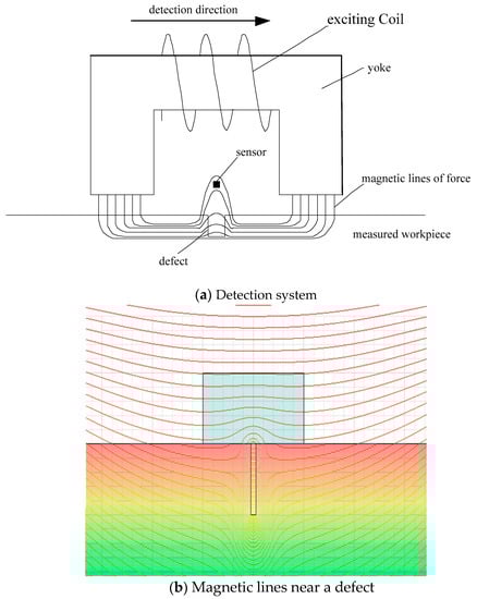
Figure 1.
MFL detection.
Figure 2 shows the section of the x-z plane near a surface defect. The defect width is 2a and the depth is b. The detection direction is also shown in Figure 2.
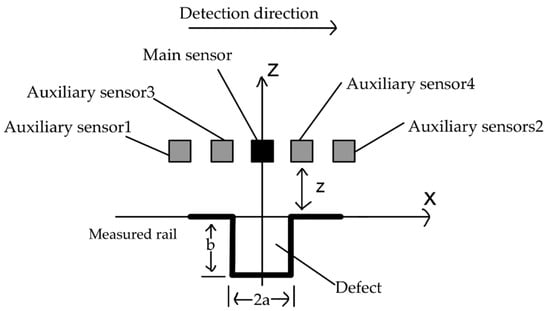
Figure 2.
The x-z plane near a defect.
The MFL field intensity of point P(x, z) above the defect is H(x, z). The x-component is Hx(x, z) and the z-component is Hz(x, z). They can be obtained by Equations (1) and (2), respectively.
where σms is the magnetic charge density of the defect side, and it is calculated by Equation (3).
In Equation (3), μ is the magnetic permeability of the material and H is the applied magnetic field strength.
According to Equations (1) and (2), the sensor signal amplitude of the same defect is different with various lift-offs. In patrol detection, when the sensor signal changes, it is difficult to distinguish whether the change is caused by a defect or the lift-off change. Due to the random interference during patrol detection, it further increases the difficulty.
If z = 1 mm, a = 1 mm, b = 1 mm, σms/2π = 1, the magnetic field distribution in the x and z directions of the defect is shown in Figure 3. It can be seen from Figure 3, as the sensor approaching the defect from far to near, the x-component of its signal increases and the z-component increases first, reaches the maximum and then decreases. When the sensor is directly above the defect, the x-component is the maximum, and the z-component is 0. As the sensor moving away from the defect, the x-component of its signal is decreases and the z-component decreases first, reaches the minimum, and then increases.
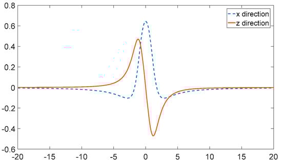
Figure 3.
MFL of a defect.
If multiple sensors are arranged in the x-direction, the relative values of their signals are regular when they pass a defect. When a sensor is directly above the defect, the x-component of its signal is more significant than that of the sensor set at other place, the z-component of its signal is more significant than those of the sensors which have passed the defect and smaller than that of the sensor which has not passed the defect yet.
The effect of lift-off on sensor signal is different from that of a defect. The smaller the lift-off, the more significant the signal, whether x or z component. If the lift-off of sensors is similar, the effect of lift-off change on the signal of each sensor is similar. Therefore, the defect signal can be distinguished from lift-off interference by the relationship among the x and z components of the sensors.
As shown in Figure 2, one main sensor and four auxiliary sensors are arranged longitudinally along the x-direction. The main sensor is used to detect the magnetic field in the x and z directions, which is set in the middle below a yoke. The other four are auxiliary sensors, numbered 1, 2, 3, and 4, which are placed on both sides of the main sensor. The auxiliary sensors 1 and 2 are used to detect the magnetic field in the x-direction, and the auxiliary sensors 3 and 4 are used to detect the magnetic field in the z-direction.
It can be proved that Hx(0, z) is the maximum and Hz(0, z) is 0. That is, when the main sensor is directly above the defect, regardless of the lift-off, the x-component of its signal is more significant than those of auxiliary sensors 1 and 2, and the z-component is smaller than that of auxiliary sensors 3 and more significant than that of auxiliary sensor 4. Therefore, the presence of defects can be determined by comparing the relative magnitudes of the sensors signals. Since this judgment is not based on the value of a sensor signal, but the relative values of different sensors signal, it is less affected by the change of the lift-off.
Obviously, the signal difference between the main sensor and the auxiliary sensors should be as large as possible to improve the accuracy of detection because of other interferences. The distance between sensors affects the difference of signals, so the space of sensors should be set reasonably.
Hx0(l) and Hz0(l) are the fitting curves of the main sensor in x and z components, Hx1(l) Hx2(l) are the fitted curves of the signals of auxiliary sensors 1 and 2 in the x-direction; Hz3(l) and Hz4(l) are the fitted curves of the signals of auxiliary sensors 3 and 4 in the z-direction. The distances between the main sensor and the auxiliary sensors 1 and 2 are both l1. The distances between the main sensor and the auxiliary sensors 3 and 4 are both l2. Obviously, if there is a defect at , Hz(l0) = 0, Hx(l0) is the maximum, Hx(l0) > Hx1(l0 − l1), Hx(l0) > Hx2(l0 + l1), Hz(l0) < Hz3(l0 − l2), Hz(l0) > Hz4(l0 + l2).
Hx(x, z0) has two minimum points from Equation (1) and Figure 3. (m1, z0) and (m2, z0) are the two points coordinates, respectively, and m1 < 0, m2 > 0. Obviously, m1 and m2 are the installation position of the auxiliary sensors 1 and 2.
When x < 0, the minimum point’s x-coordinate of Equation (4) is close to that of Equation (1). To facilitate the account, take it as m1.
The sensors are close to each other, and their lift-offs are about the same, so z0 is a constant. Take the derivative of Equation (4) to x and set it equal to 0:
Equation (5) is solved, and it is obtained that Qx(x, z0) is minimum when . Therefore, if the auxiliary sensor 1 is placed behind the main sensor and the distance is , the signal amplitude difference between the main sensor and the auxiliary sensor is the largest when the main sensor is directly above the defect.
When x > 0, the minimum point’s x-coordinate of Equation (6) is close to that of Equation (1). To facilitate the account, take it as m2.
Take the derivative of Equation (7) to x and set it equal to 0:
Equation (7) is solved, and it is obtained that Gx(x, z0) is minimum when . Therefore, if auxiliary sensor 2 is placed in front of the main sensor and the distance is , the signal amplitude difference between the main sensor and the auxiliary sensor is the largest when the main sensor is directly above the defect.
Due to the small defect, the magnetic dipole model can be introduced to simplify Equation (2) [18]:
Take the derivative of Equation (8) to x and set it equal to 0:
Equation (9) is solved, and it is obtained that Hz(x, z0) is the minimum when and Hz(x, z0) is the maximum when . Therefore, if the auxiliary sensors 3 and 4 are distributed in front of and behind the main sensor and the distance is , the signal amplitude difference between the main sensor and the auxiliary sensor is the largest when the main sensor is directly above the defect.
From the above derivation, the optimal distance from the auxiliary sensor to the main sensor is related to the size of the measured defect. In the actual measurement, the size of defects is different. Since the signal of small defects is usually weak, to ensure the detection effect, the distance between sensors is calculated according to the minimum defect size that should be detected.
In this paper, defect identification is carried out in two steps. First, the RMS of the main sensor signal is calculated as the threshold. The signal of the main sensor greater than the threshold is preliminarily determined as a defect. Otherwise, many sampling points need to be considered, and the amount of calculation is large. Then, the defects detected in the first step are further considered by the relative value of the sensors signals.
A defect is considered to exist at if conditions 1 and 3 are satisfied, or conditions 2 and 3 are satisfied; Otherwise, there is no defect at .
Condition 1.
HZ(l0) = 0.
Condition 2.
Hx(l0) is the maximum value.
Condition 3.
Hx(l0) > Hx1(l0 − l1), Hx(l0) > Hx2(l0 + l1), Hz(l0) < Hz3(l0 − l2), Hz(l0) > Hz4(l0 + l2).
is the distance from auxiliary sensors 1 and 2 to the main sensor, and is the distance from auxiliary sensors 3 and 4 to the main sensor.
Due to the random interference in the actual detection, signals without defects may meet the above conditions, resulting in misjudgment. To improve accuracy and reduce the computation, a threshold is set.
Root mean square (RMS) can not only represent the significance of the average, but also indicate the dispersion degree of the data sample. In the absence of defects, the signal amplitude is almost the same, and the RMS is small. If the signal dispersion of defects is large, the RMS is large.
Therefore, RMS is used as a threshold to eliminate the influence of the noise. Signals greater than the threshold can be initially identified as defects, and then use the above conditions to determine defects further.
4. Experimental Results and Analysis
4.1. Finite Element Simulation Results and Analysis
The finite element analysis software used in this paper is ANSYS Maxwell. A two-dimensional model is built as shown in Figure 4. The yoke is made of ferromagnetic material. The excitation coil adopts 4000 turns copper wire. The DC excitation voltage is 60 V, and the lift-off between the yoke and the rail is 20 mm. Three detection points with a lift-off of 1 mm are set up above the rail, represented by the black dots in Figure 4, the middle detection point represents the main sensor, and the other two represent the auxiliary sensors.
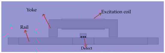
Figure 4.
Simulation Model.
In MFL detection, a defect with a different depth or width has different magnetic leakage field. Therefore, it is necessary to simulate the effect of the defect depth and width on the MFL signal.
Keep the defect width at 2 mm and change the defect depth to 1, 1.5, 2, 2.5, and 3 mm, respectively. The lift-off is 1 mm. The simulation results of the main sensor are shown in Figure 5. As the depth increases, the maximum and minimum of the signal gradually increases. When the sensors are arranged according to the minimum defect depth, the main and auxiliary sensor signal difference of a deeper defect is greater than that of the minimum depth defect.
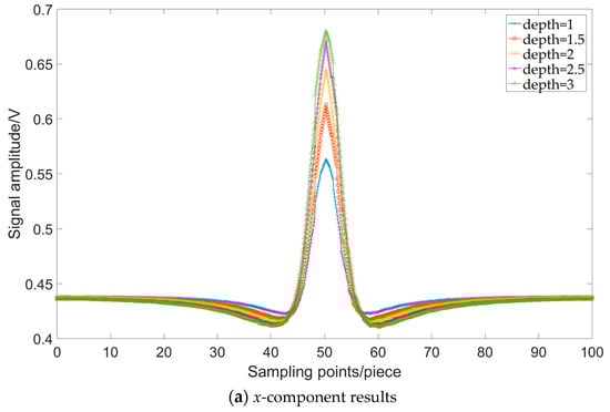
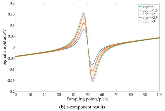
Figure 5.
Results with different depths.
Then keep the defect depth at 1 mm and change the defect width to 1, 1.5, 2, 2.5, and 3 mm, respectively. The simulation results of the main sensor are shown in Figure 6. In the x-direction, the maximum and minimum of the signal gradually increase while the defect width increased from 1 mm to 2.5 mm and the maximum value of the 3 mm wide defect decreases slightly. In the z-direction, the increase in width makes the maximum and minimum of the signal gradually increase. When the sensors are arranged according to the minimum defect width, the main and auxiliary sensor signal difference of a wider defect is greater than that of the minimum width defect.
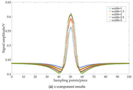
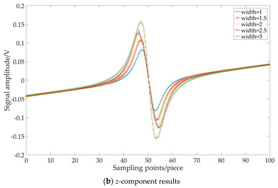
Figure 6.
Results with different width.
According to Figure 5 and Figure 6, the larger the defect, the easier it is to detect the defect. Then combined with the calculation formula, the spacing of the sensors is set according to the defect size of 2 mm in width and 1 mm in depth. The lift-off is 1 mm. The magnetic leakage field distribution of the defect is shown by the blue curve in Figure 5 and Figure 6. The optimal distance between auxiliary sensors 1 and 2 to the main sensor theory is mm, which is 3.449 mm. The optimal distance between auxiliary sensors 3 and 4 to the main sensor is mm, which is 2.236 mm. That is to say, when the main sensor is directly above the defect, the auxiliary sensors 1 and 2 are at the minimum of the blue curve in Figure 5a and Figure 6a. The auxiliary sensor 3 is at the maximum of the blue curve in Figure 5a and Figure 6a. The auxiliary sensor 4 is at the minimum of the blue curve in Figure 5b and Figure 6b.
Such arrangement of the sensors can maximize the difference of the signals among the main and auxiliary sensors when detecting a defect that is 2 mm in width and 1 mm in depth. When the depth or width of the defect increases, if the position of the sensors remains unchanged, the signal difference among the main and auxiliary sensors will also increase according to Figure 5 and Figure 6. As discussed in Section 3, the more significant the difference, the better the defect detection. Therefore, the sensors set according to small defects are also suitable for detecting large defects.
The x-component of the three detection points at different distances is analyzed. The distance of the sensors is set to 3.000 mm, 3.449 mm, 4.000 mm, respectively, and the simulation results in the x-direction are shown in Figure 7a–c.

Figure 7.
x-component simulation results with different distance.
According to the simulation results from Figure 7, with the increase of the distance between the auxiliary sensors and the main sensor, the phase difference of their signals is getting more and more significant. If the space is 3.449 mm, when the signal of the main sensor is at peak, which is indicated by the yellow line in Figure 7, the signals of the auxiliary sensors 1 and 2 are at the valley, which accords with the above conclusion.
The z-component of the sensors at different distances is analyzed. The spread of the sensors is set to 2 mm, 2.236 mm, 3 mm, respectively, and the simulation results in the z-direction are shown in Figure 8a–c:

Figure 8.
z-component simulation results with different distance.
According to the simulation results of Figure 8a–c, with the increase of the distance between the auxiliary sensors and the main sensor, the phase difference of their signals is getting more significant and more significant. If the distance between the main sensor and the auxiliary sensors is 2.236 mm, when the signal amplitude of the main sensor is 0, which is indicated by the yellow line in Figure 8, the signals of auxiliary sensors 3 and 4 are at the peak and valley, respectively, which accords with the above conclusion.
4.2. Physical Experiment Results and Analysis
4.2.1. Experimental System
An experimental system is built in the laboratory, as shown in Figure 9. The system consists of an industrial computer, a signal conditioning circuit, a DAQ card, a power supply box, and a probe. The properties of the sensor, amplifier and DAQ card are listed in Table 1. An AD620 instrumentation amplifier was used in a bias amplifier circuit. The detection speed was 2 m/s. The length and width of the sensor are both 1.5 mm. When multiple sensors are closely arranged, the minimum distance between two sensors centers is 2 mm. The probe, which consists of three sensors and an excitation device, is mounted on a detection car that is placed on the rail.
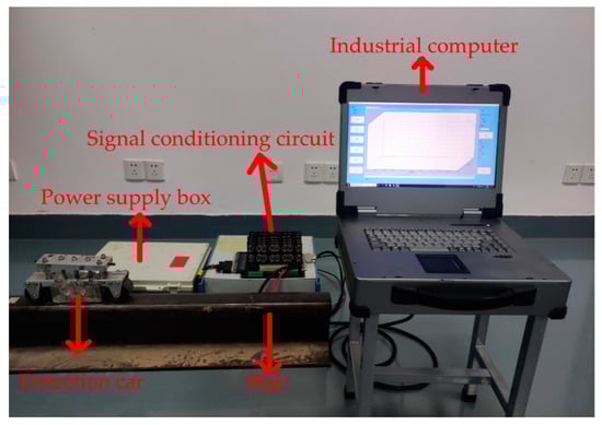
Figure 9.
Experimental system.

Table 1.
Specifications of the experimental system.
4.2.2. Experiment of the Different Spacings of the Sensors
The detection object is artificial defects, as shown in Figure 10. The distance between auxiliary sensors 1 and 2 to the main sensor is 3.4 mm and the distance between auxiliary sensors 3 and 4 to the main sensor is 2.2 mm. The direction of detection is from left to right. A wire is tied to the rail, which will change the lift-off of the handcart to simulate the vibration interference in the actual process. During detection, when no vibration is encountered, the lift-off of the sensor is fixed at 1 mm, and when the handcart wheel rolls over the wire, the lift-off will fluctuate within 1~2 mm.
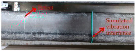
Figure 10.
A rail with an artificial defect.
Firstly, the x-components of the sensors are tested. The distance of the main sensor to auxiliary sensors 1 and 2 is set to 3.4 mm, 6.5 mm, and 10 mm, respectively. The detection results are shown in Figure 11.
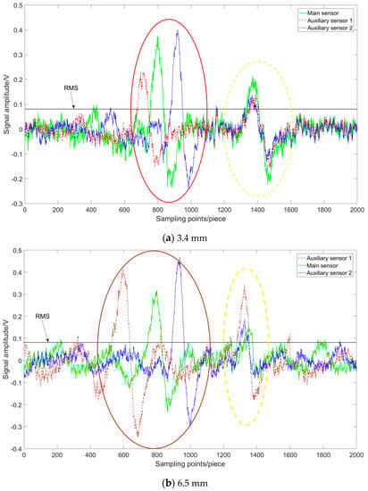

Figure 11.
x-component results with different distance.
The sensitivities of the three sensors are different, so the maximum amplitude of each signal is different. According to Figure 11a–c, as shown in the red region, the phase difference of the three signals is obvious when the sensors pass through the defect, and the difference increases with the increase of the sensor distance. In the yellow region, there is vibration interference, the amplitudes of the three signals are different, but the phases are basically the same. For only one sensor signal, the signal changes caused by vibration and defect are similar, which brings great difficulty to defect detection. The relative value of the sensors signals of a defect is different from those of a vibration. When the signal amplitude of the main sensor is the largest, the outputs of the two auxiliary sensors are smaller than that of the main sensor. There is no such phenomenon at the vibration position.
Secondly, the z-component of the sensors are tested. The distance of the main sensor to auxiliary sensors 3 and 4 is set to 2.2 mm, 4 mm, and 6 mm, respectively. The detection results are shown in Figure 12.
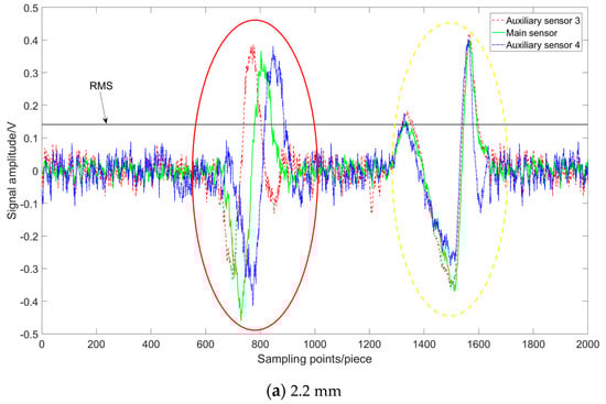
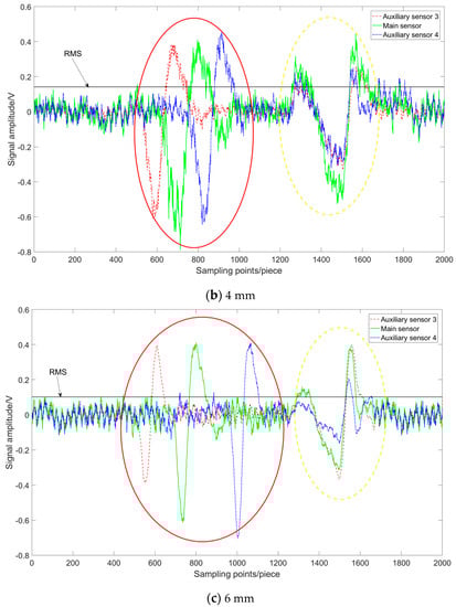
Figure 12.
z-component results with different distance.
According to Figure 12, when the sensors pass through the defect, the phase difference of the three signals increases with the increase of the sensor distance, as shown in the red region. If there is a vibration interference, the phases of the three signals are basically the same, as shown in the yellow region.
From the experimental results in x and z directions, it can be obtained that the RMS value can eliminate the influence of most system noises. At the same time, the signals at defects and vibration interference signals will be retained. Next, the phase relationship of multiple signals can be used to determine further whether it is a defect. This method can reduce the workload and misjudgment rate.
4.2.3. Experiment of the Different Defects
The dimensions of four different defects and their detection data in x and z components are shown in Figure 13 and Figure 14, respectively. The distance between auxiliary sensors 1 and 2 to the main sensor is 3.4 mm and the distance between auxiliary sensors 3 and 4 to the main sensor is 2.2 mm.

Figure 13.
x-component results with different defects.
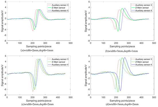
Figure 14.
z-component results with different defects.
According to Figure 13 and Figure 14, when the defect width increases, the signal phase difference will increase, and when the defect depth increases, the signal amplitude will increase. Regardless of the size of a defect, when the main sensor is directly above a defect, that is, the x-component of the main sensor signal is the largest and the z-component is 0, the x-component of the signal is significantly more significant than that of the auxiliary sensors 1 and 2; The z-component is significantly more significant than that of the auxiliary sensor 3 and smaller than that of the auxiliary sensor 4. Therefore, the proposed method can detect defects of various dimensions.
A used rail with eight artificial defects is detected, and a wire is tied to the rail also, as shown in Figure 15. The width and depth of each defect are shown in Table 2. The distance between auxiliary sensors 1 and 2 to the main sensor is 3.4 mm and the distance between auxiliary sensors 3 and 4 to the main sensor is 2.2 mm. The detection results are shown in Figure 16.
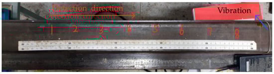
Figure 15.
A rail with multiple artificial defects.
Table 2.
The width and depth of each defect.

Figure 16.
Detection results of damage samples.
According to Figure 15 and Figure 16, the eight defects on the rail can be detected by the proposed method. The vibration interference noise can be distinguished, as shown in the yellow area part of Figure 16. As shown in Figure 17, it is the detection result of defect 2 in Figure 16. At the defect, the x-direction signal of the main sensor is the maximum, and those of the auxiliary sensors 1 and 2 are the minimum, the z-direction signal of the main sensor is zero, and the signal of auxiliary sensor 3 is the minimum, and the signal of auxiliary sensor 4 is the maximum. It can be determined that this is a defect by the method in Section 3.
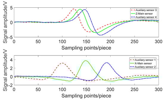
Figure 17.
Single defect.
5. Conclusions
A method is present to detect defects by using the relative value of multi-sensor signals. Sensors are set for each in x and z direction, and defects are found by comparing the amplitude of the signal of these sensors. This paper analyses the influence of the sensors distances on the signal phase is by simulation, and derives the formula of the space between the sensors under specific depth and width of a defect. In practice, the distances are calculated according to the minimum depth and width of a defect that should be detected. Simulation results show that the sensors distances calculated in this way are also suitable for the defects with more significant depth or width. The experiments show that this method can effectively distinguish the signal generated by defects from the interference caused by vibration. Of course, this method also needs further research and improvement. This paper studies the detection method for the defects of a rectangular cross-section. In the future, on this basis, we will study the detection method for defects in different cross-sections and directions.
Author Contributions
Conceptualization, Y.J. and S.Z.; methodology, Y.J.; software, S.Z.; validation, Y.J., S.Z. and K.J.; formal analysis, Y.J.; investigation, K.J.; resources, S.Z.; data curation, S.Z.; writing—original draft preparation, S.Z.; writing—review and editing, Y.J.; visualization, K.J.; supervision, P.W.; project administration, P.W.; funding acquisition, P.W. All authors have read and agreed to the published version of the manuscript.
Funding
This work was funded by the National Key R&D Program of China (2018YFB2100903) and the Fundamental Research Funds for the Central Universities (No. NJ2020014).
Institutional Review Board Statement
Not applicable.
Informed Consent Statement
Not applicable.
Conflicts of Interest
The authors declare no conflict of interest.
References
- Zhang, H.; Song, Y.N.; Wang, Y.N. Review of rail defect non-destructive testing and evaluation. Chin. J. Sci. Instrum. 2019, 40, 11–25. [Google Scholar]
- Zhang, Q.; Zou, D.Q.; Yang, Q.Q. Research and analysis of damaged morphology and structure on the head of switch rail. Yejin Fenxi/Metall. Anal. 2019, 39, 23–28. [Google Scholar]
- Alahakoon, S.; Sun, Y.Q.; Spiryagin, M.; Cole, C. Rail Flaw Detection Technologies for Safer, Reliable Transportation: A Review. J. Dyn. Syst. Meas. Control 2018, 140, 0208011–02080117. [Google Scholar] [CrossRef]
- Popović, Z.; Radović, V.; Lazarević, L. Rail inspection of RCF defects. Metalurgija 2013, 52, 537–540. [Google Scholar]
- Liu, Y. Theoretical and Experimental Research on Wheel-Rail Contact Characteristics and Rail Damage Factors. Ph.D. Thesis, Lanzhou Jiaotong University, Lanzhou, China, 2016. [Google Scholar]
- Hong, Q.P.; Quang, T.T.; Duy, T.D.; Tran, Q.H. Importance of Magnetizing Field on Magnetic Flux Leakage Signal of Defects. IEEE Trans. Magn. 2018, 54, 1–6. [Google Scholar]
- Bevan, A.; Klecha, S. Use of magnetic flux techniques to detect wheel tread damage. Proc. Inst. Civ. Eng. 2016, 169, 330–338. [Google Scholar] [CrossRef]
- Antipov, A.G.; Mmarkov, A.A. Detectability of Rail Defect by Magnetic Flux Leakage Method. Russ. J. Nondestruct. Test. 2019, 55, 277–285. [Google Scholar] [CrossRef]
- Sun, Y.; Liu, S.; Ye, Z.; Chen, S.; Zhou, Q. A Defect Evaluation Methodology Based on Multiple Magnetic Flux Leakage (MFL) Testing Signal Eigenvalues. Res. Nondestruct. Eval. 2016, 27, 1–25. [Google Scholar] [CrossRef]
- Okolo, C.K.; Meydan, T. Finite element method and experimental investigation for hairline crack detection and characterization. Int. J. Appl. Electromagn. Mech. 2019, 59, 1203–1211. [Google Scholar] [CrossRef]
- Al-Naemi, F.I.; Hall, J.P.; Moses, A.J. FEM modelling techniques of magnetic flux leakage-type NDT for ferromagnetic plate inspections. J. Magn. Magn. Mater. 2006, 304, e790–e793. [Google Scholar] [CrossRef]
- Yang, L.N.; Geng, H.; Gao, S.W. Study on the establishment process and influence factors of high-speed magnetic flux leakage testing. Chin. J. Sci. Instrum. 2019, 40, 1–9. [Google Scholar]
- Antipov, A.G.; Markov, A.A. Evaluation of transverse cracks detection depth in MFL rail NDT. Russ. J. Nondestruct. Test. 2014, 50, 481–490. [Google Scholar] [CrossRef]
- Yang, L.J.; Geng, H.; Gao, S.W. Study on high-speed magnetic flux leakage testing technology based on multistage magnetization. Chin. J. Sci. Instrum. 2018, 39, 148–156. [Google Scholar]
- Tsukada, K.; Majima, Y.; Nakamura, Y.; Yasugi, T.; Song, N.; Sakai, K.; Kiwa, T. Detection of Inner Cracks in Thick Steel Plates Using Unsaturated AC Magnetic Flux Leakage Testing with a Magnetic Resistance Gradiometer. IEEE Trans. Magn. 2017, 53, 1–5. [Google Scholar] [CrossRef]
- Okolo, C.K.; Meydan, T. Pulsed magnetic flux leakage method for hairline crack detection and characterization. Aip Adv. 2017, 8, 047207. [Google Scholar] [CrossRef]
- Jia, Y.L.; Liang, K.W.; Wang, P. An Enhancement Method of Magnetic Flux Leakage Signals for Rail Track Surface Defect Detection. IET Sci. Meas. Technol. 2020, 14, 711–717. [Google Scholar] [CrossRef]
- Wu, J.; Yang, Y.; Li, E.; Deng, Z.; Kang, Y.; Tang, C.; Sunny, A.I. A High-Sensitivity MFL Method for Tiny Cracks in Bearing Rings. IEEE Trans. Magn. 2018, 54, 1–8. [Google Scholar] [CrossRef]
- Azad, A.; Kim, N. Design and Optimization of an MFL Coil Sensor Apparatus Based on Numerical Survey. Sensors 2019, 19, 4869. [Google Scholar] [CrossRef] [Green Version]
- Liu, S.; Sun, Y.; Deng, Z.; He, L.; Gu, M.; Liu, C.; Kang, Y. A novel method of omnidirectional defects detection by MFL testing under single axial magnetization at the production stage of lathy ferromagnetic materials. Sens. Actuators A Phys. 2017, 262, 35–45. [Google Scholar] [CrossRef]
- Liu, X.C.; Wang, Y.J.; Wu, B.; Zhen, G.; Cunfu, H. Design of Tunnel Magnetoresistive-Based Circular MFL Sensor Array for the Detection of Flaws in Steel Wire Rope. J. Sens. 2016, 2016, 35–45. [Google Scholar]
- Wu, D.H.; Liu, Z.T.; Su, L.X. New MFL detection method based on differential peak extraction using dual sensors. Chin. J. Sci. Instrum. 2016, 37, 1218–1225. [Google Scholar]
- Wu, D.H. A Novel Non-destructive Testing Method by Measuring the Change Rate of Magnetic Flux Leakage. Nondestruct. Eval. 2017, 36, 24. [Google Scholar]
- Sun, Y.H.; Kang, Y.H. Magnetic mechanisms of magnetic flux leakage nondestructive testing. Appl. Phys. Lett. 2013, 103, 184104. [Google Scholar] [CrossRef]
Publisher’s Note: MDPI stays neutral with regard to jurisdictional claims in published maps and institutional affiliations. |
© 2021 by the authors. Licensee MDPI, Basel, Switzerland. This article is an open access article distributed under the terms and conditions of the Creative Commons Attribution (CC BY) license (https://creativecommons.org/licenses/by/4.0/).