Abstract
This article evaluates a recently introduced algorithm that adjusts each dimension in particle swarm optimization semi-independently and compares it with the traditional particle swarm optimization. In addition, the comparison is extended to differential evolution and genetic algorithm. This presented comparative study provides a clear exposition of the effects introduced by the proposed algorithm. Performance of all evaluated optimizers is evaluated based on how well they perform in finding the global minima of 24 multi-dimensional benchmark functions, each having 7, 14, or 21 dimensions. Each algorithm is put through a session of self-tuning with 100 iterations to ensure convergence of their respective optimization parameters. The results confirm that the new variant is a significant improvement over the traditional algorithm. It also obtained notably better results than differential evolution when applied to problems with high-dimensional spaces relative to the number of available particles.
1. Introduction
Particle swarm optimization (PSO) algorithms are reputed for optimizing complex multidimensional problems with a balanced trade-off between reliability of convergence and computational efficiency. PSO relies on momentum, local/personal best attraction, and global best attraction to find a global optima. Although PSO tends to be slightly slower than differential evolution (DE), it can produce similar or even slightly better convergence rates depending on the problem at hand [1,2]. PSO also tends to be faster and more efficient than genetic algorithms (GAs), which rely heavily on random mutation and cross-over.
The work reported in this article builds on prior work where PSO was modified to optimize each dimension semi-independently [3]. This variant, called dimension-wise particle swarm optimization (DPSO), aims to increase the convergence reliability at the cost of some additional time complexity. The focus of the original article [3] was on how varying the ratio of particles to dimensions and per-dimension sensitivity—henceforth referred to as ill-conditioning—affected the algorithm’s ability to find the global optimum. These evaluations were carried out with scarce populations, i.e., with more dimensions than particles, which increased the difficulty and importance of exploration. The same article also introduced self-tuning as a method of PSO parameter selection. These configurations are carried over to this work with some changes in the rules, an inclusion of DE and GA in the evaluation, and an increase in the number of functions to be optimized.
An in-sample evaluation with some degree of similarity to each out-of-sample function is used for each optimizer’s parameter optimization process. The most suitable optimizer parameters are determined using self-tuning. This way, the algorithm of interest can explore and change its parameters during the in-sample test should it find a statistically better set w.r.t. fitness. For the out-of-sample tests, each algorithm must rely on the generally optimized parameters derived from the self-tuning process. The results are evaluated based on the statistical mean and standard deviation of each algorithm’s global optimum results for the 24 problem functions used. These benchmark functions are composed of 7-, 14-, and 21-dimensional spaces with randomly generated offsets, ill-conditioning, rotation, and overlaps. To ensure the results are reliable, each problem function is randomly generated and evaluated 30 times.
Related Work
PSO has a wide range of modifications, which address specific aspects of the algorithm or the problem of interest. PSO can be improved by integrating other algorithms into its process—such as neural networks and support vector machines—or by modifying the fundamental rules for particle movement [4,5,6,7,8]. For relatively high dimensional problems, it is usually preferred to selectively optimize a subset of dimensions at a time [9]. By occasionally changing the subset, progressive convergence towards the overall global optimum can be improved.
DPSO differs from other variants such as dual gbest PSO (DGPSO) in that it does not rely on preprocessing steps to identify, order, and select the dimensions with the greatest sensitivity [9]. A simpler method of feature selection borrows from the GA, where crossover is used to combine the particle’s current location, a predetermined relevant feature vector, the global best position, and its local best position. However, this approach uses a look-ahead approach, evaluating the three candidate locations before choosing the best one as the new individual, effectively tripling the population size during evaluation [10]. PSO with an enhanced learning strategy and crossover operator uses a weighted sum of local bests over all particles based on a normalized fitness distribution to achieve variations in attractor locations [11]. DGPSO’s approach can be described as a divide-and-conquer approach, while PSO with crossover hybridizes features from GA into PSO. These methods improve PSO’s ability to find the optimum; however, many come at the expense of notably larger preprocessing requirements or by superficially increasing the population size. The aim of DPSO is to improve the fitness with relatively small increases in computational demand by limiting the scale of the modifications. DPSO’s approach is less complicated, randomly selecting dimensions to apply global and local best attractions based on a fixed probability value. The selection of dimensions is not of a fixed number, nor is it based on pre-processed information about the local search space, thus maintaining a relatively low computational cost. The binary nature of DPSO’s attractors is closer to casting a net-like structure of potential attraction points on the search space solely based on the particles’ current location and the location of the local and global best points; i.e., it does not require pre-processing or a look-ahead feature.
The velocity limitations imposed on DPSO are similar to the boundary restrictions of the population migration PSO’s (PMPSO). However, DPSO’s limits do not change in scale over time and only restrict each particle’s maximum viable search space for the next iteration relative to its current location [12]. Velocity restriction-based improvised PSO (VRIPSO) uses a dynamic method of limiting velocity and relies on an escape velocity mechanism to explore beyond its velocity limit [13]. Alternatively, DPSO warps individuals who appear to be stagnating, while VRIPSO occasionally allows particles to escape the imposed velocity limit. Warping has been applied to all algorithms in this article as a general rule to ensure that it does not become a primary difference in results. Although VRIPSO’s approach may allow for faster convergence in some circumstances, DPSO’s warping condition recycles particles to increase the exploration of dimensions that may not have been sufficiently covered.
Tabu search PSO has an interesting feature, where the fitness results of particles and the respective locations are saved for a specified number of iterations [8]. This type of logging has been applied for all algorithms covered in this article but without removing older records. By recording the fitness of a location for later, it is possible to skip the function evaluation step and, over time, to significantly reduce the time spent on iterations with repeated positions. An element of reserving the position was also included in all algorithms to ensure that multiple particles on the same position would only require one shared evaluation.
Another feature found in VRIPSO is that it adjusts momentum over time [13]. Continuous PSO has a more in-depth version of this momentum feature in that it determines a gradient by which to adjust the momentum factors, encouraging movement in directions with greater improvements and not just in the current direction [14]. Though these dynamic methods are appealing, DPSO was limited to using random noise injection, which can either dampen or excite the particle’s movement irrespective of the perceived gradient or its direction of travel. These random perturbations allow for greater degrees of exploration along the dimensions lacking in representation or for which movement has stagnated. Given that this research is interested in solving high-dimensional problems with relatively sparse population sizes, it is important to ensure that particles do not restrict themselves to a subset of searchable dimensions while neglecting the rest.
2. Algorithms
For all algorithms, the local best position is the individual’s recorded best optimal value such that, in the case of minimizing the reward ,
where N is the number of individuals used in the algorithm. The conditional replacement of the position when serves to allow for a possibility of equivalent locations to replace the current attraction point. This comparison can also be made for the global best by evaluating across each individual i of the current iteration such that
The reward r is an evaluation of fitness w.r.t. the parameters p when they are applied to the problem of interest. As the chosen problems are evaluated over 30 runs, r is the average plus standard deviation, to not only prefer parameters that perform well on average, but also give some preference to parameters that give consistent results. By recording with six decimal points of resolution and a range for problem functions and for self-tuning algorithms, the search spaces become partially discretized and ensure the recorded values are precise in their outcomes. This setup assures that dependencies in the reward do not arise from rounding off the seventh decimal place, and allows for some extrapolation into more granular ranges such as integers. As the algorithms are iterating over a relatively long series of optimization steps, a log of fitness values is included to save processing time at the expense of memory. In the situation where the algorithm fails to process the current position, the fitness value is set to . Should a given particle stagnate, i.e., when , the individual is warped to a new random position, maintaining a degree of random exploration.
2.1. Traditional PSO
In the traditional PSO algorithm, each individual has a velocity and position update method [15]
and
respectively, where is the momentum constant, and and are the global and local attraction strengths. is a randomly generated value from a uniform distribution within the range . varies the degree of attraction to the respective best value every iteration up to and , respectively. The parameter labels have been changed for ease of equating to data arrays in code. This is applied to all later algorithms as well, however, these parameters are entirely independent.
Velocity and position vectors are subject to the dimension-wise limitation
and
Allowing particles to bounce off the upper and lower limits maintains a degree of activity, preventing early termination of exploration due to boundary collisions. Additionally, given that the position is stopped at the respective limit, a measure of performance at the said limit will still be obtained. The general process flow for PSO is shown in Figure 1a. The velocity calculation time complexity is , position updates are , and each dimension limit check is , resulting in a total time complexity per iteration of .
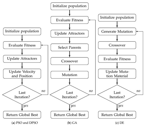
Figure 1.
Flow diagrams depicting the process of each algorithm.
2.2. Dimension-Wise PSO
The Dimension-wise PSO (DPSO) algorithm has been designed with the intention of handling relatively large dimensional spaces with a sparse population size. This is accomplished by determining the global and local attraction points separately for each dimension. DPSO’s velocity is defined as
and is also subject to dimension-wise limitations
followed by Equation (5). As with PSO, the individual’s position update relies on Equation (4) subject to Equation (6).
Percent noise injection—regulated by —is used as a precaution to improve variations in movement and increase the likelihood of escaping from local minima without causing a large change in course. Noise injection replaces the random values affecting attractor strengths and allows it to have an effect independent of a particle’s distance from the optima. Visually, it can be likened to roughening a surface dependent on the speed of a ball rolling down its surface, causing the said ball to deviate from a trivial path. The trajectory and speed are often disrupted, but the general direction of travel is not necessarily changed as it has three other elements that are largely responsible for determining velocity, i.e., momentum, global best attraction, and local best preference.
The velocity limit, , partially opposes the effect of percent noise injection, as it attempts to restrict the overshooting caused by an excessive build up of momentum and attractive strength along a given dimension. Situations where a particle builds up too much momentum and is slingshot further away from the known optimal locations can help with increasing diversity in exploration, but scattering particles away from the optimal attractors can also impair the rate of convergence [16]. To prevent an excessive expansion in the required search parameters, is simplified to
where is the percentage of a given dimension’s span a particle can traverse in one iteration, and and are the position boundaries bracketing the valid range of exploration along the given dimension.
The primary change that gives DPSO the ability to search on a per-dimension basis is that, in Equation (7), the uniform random attraction values are replaced with probabilistic binary values, and , respectively. These values determine if the individual should move toward the respective best position of a given dimension. The activation of and can be described as
where and denote the respective probability of activation. It must be stressed that and are evaluated on a per-dimension basis, as opposed to being a single value applied to each dimension. Although this discretized approach reduces the coverage of points between the two known best locations, it increases the exploration of points in the surrounding neighborhood (see Figure 2). When momentum and noise injection are accounted for, the individual is less likely to become fixated on a single vector and can partially explore the area around each point. Without noise or momentum, the probability of moving to a given point is based on the products of , , , and/or for each dimension. For the top-left example in Figure 2, if the lower ‘×’ marks the global optimum, the point in the top left corner would have the following transition probability
where and denote the dimension with which the binary attractor is associated. The probability of transitioning to the global optimum’s mark is
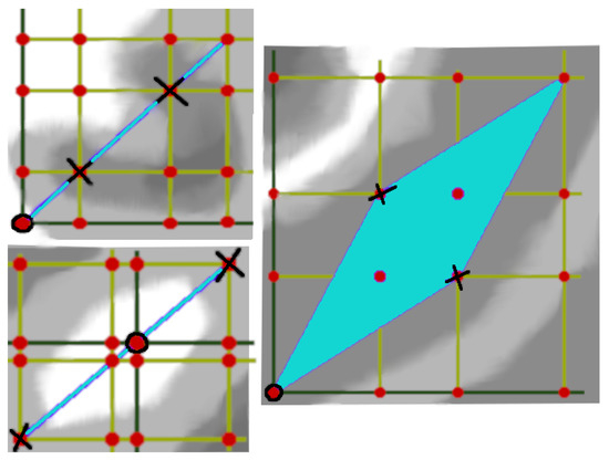
Figure 2.
The difference between exploitation with PSO (blue envelope) and DPSO (red points on the grid).
As with the traditional PSO, when and are reduced, the scale of movement, i.e., the grid size, is reduced. Momentum skews the final landing point in the direction of motion, while noise injection causes each potential attractor point to represent the center of a distribution. It is worth noting that DPSO values and make this variant the closest possible form to the original PSO, where the key differences are the attraction random values. The general process flow for DPSO is identical to PSO (see Figure 1a). The velocity calculation time complexity is , binary attractor selections are , position updates are , and each dimension limit check is , resulting in a total time complexity per iteration of —approximately more than PSO.
2.3. Genetic Algorithm
The Genetic Algorithm (GA) is very different from PSO in its method of optimization, as it does not rely on momentum or points of attraction. Instead, it uses the fitness of individuals from the last generation [17]. The first step of modifying the parameters is selecting parents. In this study, it is carried out through a roulette-style competition without replacement, where each individual’s fitness is determined by the following
where returns the number of individuals who obtained the current minimum fitness, which allows the fitness distribution to approach a uniform distribution as more individuals produce equivalent fitness values.
As there is no order on the resulting list of parent indices, they are considered sufficiently mixed. These parents are used in pairs to produce the kth child
where is the modulus division of k by the number of selected parents q. parent1 and parent2 are the indices of the chosen parents whose genes are and , respectively.
The number of parents permitted to produce offspring is defined by
where is the percent population allowed to reproduce. The percent replacement is determined by , i.e., the population that was not selected is replaced to minimize redundant evaluations. After the parents are selected, crossover occurs with
where with random permutation and otherwise. G is the length of the genome, and denotes a random choice of X elements of G without replacement, while is with replacement. Gene mutation for each child is determined by a random permutation with replacement , where is the maximum allowed percent mutation a genome can undergo (the minimum is one mutated genome). For each unique gene/dimension selected for mutation, a uniform random value within the respective limits is applied. The general process flow for GA is shown in Figure 1b. The individual fitness calculation time complexity is , parent selection which shuffles and fully utilizes the current population is , a random permutation of the genes for each child is , crossover with full replacement is , mutation is , and each dimension limit check is , resulting in a total time complexity per iteration of .
2.4. Differential Evolution
Differential Evolution (DE) tends to be faster in processing due to its relative simplicity. A key difference from PSO and GA is that DE mutates its population before evaluating the fitness of its individuals [18]. The first step is choosing a random permutation for the genetic material to be used for mutation
where is the degree of mutation that can be imposed on the base material provided by sample ‘a’. After a mutant is generated, each gene/dimension has the possibility of going through crossover—determined by the crossover probability —where the respective mutated gene is clipped to fit within the dimension’s limits and applied to the targeted individual, i.e., . If no genes are selected for crossover, one is selected at random.
The general process flow of DE is shown in Figure 1c. The random permutation of three genetic sources has a time complexity is , mutated gene production is , crossover using a random permutation is , and each dimension limit check is , resulting in a total time complexity per iteration of .
3. Methodology
The configuration for this experiment is such that the algorithm is assigned an initial estimate of the best parameter combination, which is randomly seeded with one of the individuals to be evaluated. This algorithm (Alg1) is set to optimize 5 particles for up to 100 iterations. Thirty copies of the algorithm (Alg2) are generated as the problem function, each optimizing 5 particles for up to 500 iterations. For each of these optimized algorithms, 30 randomly offset and ill-conditioned copies of the in-sample problem function are set to be optimized. Alg2’s average global optimum result across these 30 copies plus the standard deviation is taken as the algorithm’s measure of fitness during self-tuning. The outcome of evaluating the fitness of Alg2, i.e., its final global optimum result, is used as follows: if it is better than what was recorded for the global optimum in Alg1, the parameters used by Alg1 are updated to those of Alg2 before moving on to the next iteration. After self-tuning, the optimal parameters are applied to the algorithm again with 30 separate runs of the out-of-sample function problems. The out-of-sample optimization uses 5 individuals and lasts for 1000 iterations without allowance for early termination. The mean results of the out-of-sample global best logs are recorded for plotting and the final mean and standard deviation values are recorded for tabulation.
3.1. Self-Tuning
Self-tuning is a form of bootstrapping, where the algorithm attempts to improve its own parameters based on its relative improvement in optimizing a problem [19]. Granted, it is inefficient to self-tune on the problem of interest as this will likely result in having found the global optimum several times over. Therefore, it is preferred to self-tune using a simpler approximation of the out-of-sample problem(s) as an in-sample training step. This allows the algorithm parameters to be generally optimized for any problem similar to the in-sample function. For self-tuning to be effective, the in-sample problem must be a close approximation of the out-of-sample function set. In the case where the out-of-sample set only has one function, the in-sample function must at least be sufficiently simplified to make the additional evaluation steps worthwhile. In contrast to some alternative self-tuning methods, an external approach does not require specialized modifications or rules to adjust the parameters on the fly [20,21].
3.2. Function Problems
The base problem functions used as benchmarks are: Elliptical (scale: 500), Ackley (scale: 32), Rosenbrock (scale: 7.5; offset: 1.5), Rastrigin (scale: 5.12), Drop-wave (scale: 5.12), Zero-sum (scale: 10), and Salomon (scale: 100) [22,23]. For 2 to 3 dimensions, most of these functions would be considered somewhat challenging, as they have many local minima. To add complexity to each problem, random offsets (up to off center) and ill-conditioning (up to 10 times the scale), rotations, and partial-separability ( overlap) were applied in steps as shown in Table 1 [24]. The dimensions shown in the table are for the 14D problem; however, these steps were similarly carried out for 7D and 21D problems. Ill-conditioning, rotation, and overlap effects were applied to all 7, 14, and 21 dimensions, respectively, while the 4 copies of each function had independently allocated dimensions. For the cases of overlap and rotation, some of these functions are partially dependent on the same inputs, further complicating the search process.

Table 1.
The list of functions evaluated on for each algorithm.
4. Results
The resulting optimal parameters after self-tuning on are shown in Appendix A (Table A1, Table A2 and Table A3). For each algorithm, the final optimal parameters tended to be found well before reaching the limit of 100 iterations. In all cases, DPSO has shown to be a significant improvement from PSO, which was consistently in the last place. The resulting fitness in Table A4, the normalized fitness and per-problem rank in Table 2, and the plots shown in Figure A1, Figure A4, Figure A7 and Figure A10, suggest that DPSO is capable of outperforming DE and GA in overall fitness with a margin of approximately when using five particles on seven-dimensional problems. For 14 dimensions, Table 3 and Table A5, as well as Figure A2, Figure A5, Figure A8 and Figure A11, show that, although DPSO easily bests the GA results and despite only placing third or fourth in 6 of the 24 problem functions, it underperforms w.r.t. DE with a margin of . Rank Factor is the average result of the normalized fitness divided by the smallest average normalized fitness. The Normalized fitness in Table 2, Table 3 and Table 4 are the fitness results scaled for ease of comparison.
Table 2.
Normalized fitness w.r.t. each function problem with 7 dimensions and the resulting ranking: rank 1 (best), rank 2, rank 3, and rank 4.
Table 3.
Normalized fitness w.r.t. each function problem with 14 dimensions and the resulting ranking: rank 1 (best), rank 2, rank 3, and rank 4.
Table 4.
Normalized fitness w.r.t. each function problem with 21 dimensions and the resulting ranking: rank 1 (best), rank 2, rank 3, and rank 4.
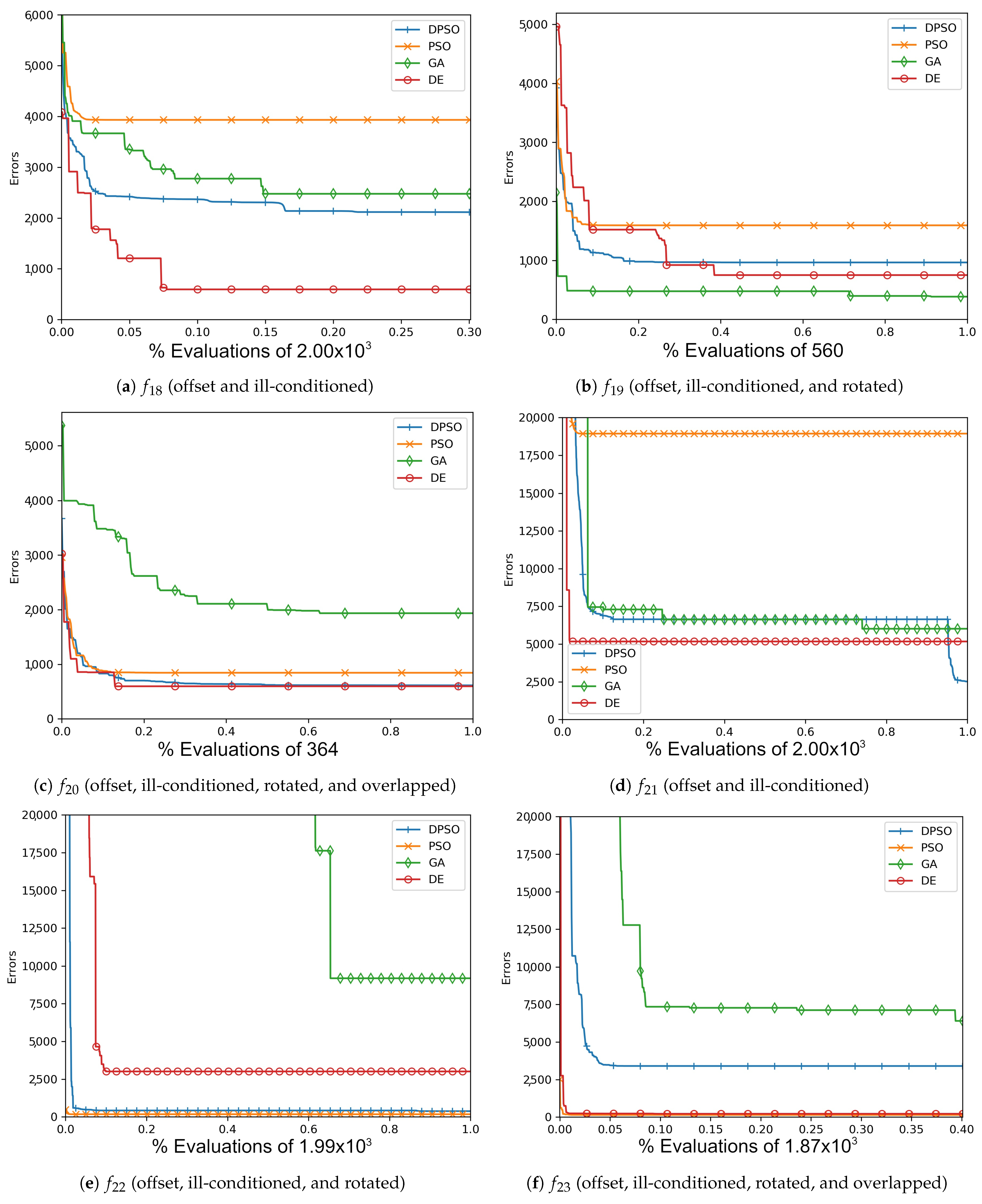
Increasing the dimensions to 21, DPSO’s overall fitness is notably better with respect to Table 4 and Table A6 relative to the ranked second DE with a margin of more than . The gradual improvements shown in Figure A3, Figure A6, Figure A9 and Figure A12 also suggest that DPSO’s ability to make gradual improvements was not severely hindered by the small ratio of particles to dimensions. Given that the standard deviation is relatively small compared to the mean fitness, the algorithms’ final rankings are expected to be reliable for the applied out-of-sample functions and chosen parameters.
The results of this experiment show that DPSO and DE can be optimized through self-tuning given a sufficient number of iterations and that they both demonstrate satisfactory results. The tuned parameters allow these algorithms to remain largely effective when the target problem deviates from the in-sample function, i.e., when they are able to self-tune on an approximation of the out-of-sample problems and can be expected to perform well. Given the fact that the rules were applied equally to all algorithms, the primary cause for improvement in DPSO over PSO is the use of dimension-wise updates. A likely reason why a number of fitness results are relatively large is that ill-conditioning scales up the dimensional range, making it harder to find the global optimum. Regardless, every algorithm was able to demonstrate some improvement in each problem, e.g., ending with a fitness of is a significant improvement when starting with . It is interesting that the Ellipse problems had the worst performance results despite the relative simplicity of its surface—likely attributed to the exponential nature of each axis. PSO and DPSO have momentum factors that can cause them to overshoot or orbit the minima, but this problem does not exist for DE and GA. The likely factor that makes some of these problems more difficult for DE and GA is that the population size, which they rely on for diversity, is relatively small compared to the number of dimensions. This way, they are entirely reliant on warping and mutation to increase the variety of candidate solutions. Without randomly generating new genomes, they can only make do with trying to improve on the dimensions for which there is a sufficient variety of overall fit individuals to experiment on. From Figure A1, Figure A2, Figure A3, Figure A4, Figure A5, Figure A6, Figure A7, Figure A8, Figure A9, Figure A10, Figure A11 and Figure A12, it is apparent that most algorithms tend to converge or approach convergence within the first 500 iterations, with relatively small improvements thereafter. The last improvement in the global optimum is given at x-axis value 1.0 in the plots—shown in Table A4, Table A5 and Table A6—but data with next to no improvement at the end were removed to improve clarity where possible. The sudden improvement given by DPSO may be due to the fact that the dimension-wise activation of attractors is similar in principle to the crossover method found in GA and DE.
A separate test without logging was conducted on the elliptical function () to analyze the computational costs of these algorithms (given in Table 5). As expected, DPSO is slightly more demanding than PSO by approximately 300 bytes (4.7%) for seven dimensions, further diminishing to 3.6% and 3.2% for 14 and 21 dimensions, respectively. Compared to GA and DE, both DPSO and PSO are notably more memory demanding.
Table 5.
The Computational costs in terms of average memory and time for each dimension size on the elliptical problem.
In terms of execution time, DPSO requires a few milliseconds more per iteration than GA and DE. The time lapse was determined by the average execution time to complete one iteration over 200 iterations and 21 dimensions. Given that the time complexities for GA and DE are similar and smaller than for PSO and DPSO, it is likely that some areas of code are not fully optimized even though the base code was the same and care was taken to minimize deviations from the base. In exchange for a slightly larger processing time relative to the other algorithms, DPSO was able to reduce the rate at which its ability to converge worsened when the disparity between population and search-space dimensionality increased.
There are several components of the DPSO algorithm that contribute to its execution time. Their individual contributions can be measured by recording the corresponding time lapse. The time required for PSO to calculate momentum followed by the time lapse for local and global attraction forces can be compared to DPSO’s momentum plus noise injection and dimension-wise attraction forces. The difference in calculation time for momentum (>1 μs) versus momentum plus noise injection (36 μs) and the regular attraction (7 μs) versus the dimension-wise attraction (116 μs) calculations is larger than expected. A notable portion of this increase can likely be attributed to DPSO relying on a for-loop to perform its per-dimension calculations, while PSO is able to exploit the optimizations given by the numpy library. Regardless, the velocity update steps for DPSO are expected to take more time given that the attractors are decided on a per-dimension basis.
5. Conclusions and Future Work
This article examines the recently introduced dimension-wise particle swarm optimization (DPSO) algorithm and compares its performance with other commonly used metaheuristic optimization systems. Specifically, it compares the statistical mean of the global fitness values for DPSO, PSO, GA, and DE in a two-step process: in-sample tuning and out-of-sample evaluation. The optimal parameters for each algorithm were selected by applying self-tuning while evaluating 30 independent runs of a generic in-sample problem that approximated the set of all functions used for evaluation. To evaluate the performance, each algorithm was tested on 24 separate problems, and the mean and standard deviation were obtained from 30 separate runs of each for 7, 14, and 21 dimensions. The obtained results show that DPSO performs better than DE, PSO, and GA when the population is sparse w.r.t the number of dimensions to be explored.
In future work, it may be worth incorporating other methods such as Adaptive PSO to reduce the number of parameters that must be tuned. It may also be interesting to investigate other options for rules on warping particles and setting the population size as one of the adjustable parameters. To better grasp the benefits of DPSO, it would also be worth comparing this algorithm with more state-of-the-art variations in PSO such as Dual Gbest PSO without regard for the computational costs. Given that there is no conflict with momentum degradation methods such as the one found in continuous PSO w.r.t. the changes made in DPSO, integrating them into DPSO may allow for further improvements in fitness with minimal addition to computational costs [9].
Author Contributions
Conceptualization, P.M.; methodology, J.S.; software, J.S.; investigation, J.S.; resources, P.M.; writing—original draft preparation, J.S.; writing—review and editing, P.M.; supervision, P.M.; project administration, P.M.; and funding acquisition, P.M. Both authors have read and agreed to the published version of the manuscript.
Funding
This research was funded by the Natural Sciences and Engineering Research Council (NSERC) of Canada grant number RGPIN-2017-05866 and by the Government of Alberta under the Major Innovation Fund, project RCP-19-001-MIF.
Conflicts of Interest
The authors declare no conflict of interest.
Symbols
The following symbols are used in this manuscript:
| Position of a particle at time t | |
| Velocity of a particle at time t | |
| r | Location fitness on the problem surface at a given point/time |
| N | The total number of particle/individual used |
| D | The total number of dimensions in the search space |
| i | An arbitrary particle/individual of the current iteration |
| t | Time step/iteration/generation |
| local | Denoting local attractor information |
| global | Denoting global attractor information |
| A uniform randomly generated number within the range | |
| An algorithm parameter designated for tuning | |
| Binary decider for attractors and crossover |
Appendix A. Additional Tables and Graphs
Table A1.
Global best self-tuning parameters for 7 dimensions.
Table A1.
Global best self-tuning parameters for 7 dimensions.
| DPSO | c0 | c1 | c2 | c3 | c4 | c5 | c6 |
| 0.862056 | 0.859008 | 0.620299 | 0.526893 | 0.103819 | 0.986512 | 0.801248 | |
| PSO | |||||||
| 0.107710 | 0.741607 | 0.492210 | |||||
| GA | |||||||
| 0.974085 | 0.558012 | ||||||
| DE | |||||||
| 0.251732 | 0.000000 | ||||||
DE is forced to choose one parameter to crossover.
Table A2.
Global best self-tuning parameters for 14 dimensions.
Table A2.
Global best self-tuning parameters for 14 dimensions.
| DPSO | c0 | c1 | c2 | c3 | c4 | c5 | c6 |
| 0.507646 | 0.438668 | 1.000000 | 0.308361 | 1.000000 | 0.655705 | 0.970521 | |
| PSO | |||||||
| 0.649608 | 0.594950 | 0.175723 | |||||
| GA | |||||||
| 0.899098 | 0.233414 | ||||||
| DE | |||||||
| 0.470144 | 0.544929 | ||||||
Table A3.
Global best self-tuning parameters for 21 dimensions.
Table A3.
Global best self-tuning parameters for 21 dimensions.
| DPSO | c0 | c1 | c2 | c3 | c4 | c5 | c6 |
| 0.734627 | 0.712416 | 0.891312 | 1.000000 | 0.767508 | 0.853393 | 0.786354 | |
| PSO | |||||||
| 0.715330 | 0.386808 | 0.897650 | |||||
| GA | |||||||
| 0.390245 | 0.092636 | ||||||
| DE | |||||||
| 1.000000 | 0.532237 | ||||||
Table A4.
Fitness w.r.t. each function problem with 7 dimensions and the resulting ranking: rank 1 (best), rank 2, rank 3, and rank 4.
Table A4.
Fitness w.r.t. each function problem with 7 dimensions and the resulting ranking: rank 1 (best), rank 2, rank 3, and rank 4.
| Function | DPSO | PSO | GA | DE |
|---|---|---|---|---|
| Ave | 1.234 × 10 | 1.424 × 10 | 8.956 × 10 | 3.439 × 10 |
| Std | 2.252 × 10 | 2.910 × 10 | 0.000 | 1.342 × 10 |
| Ave | 1.641 × 10 | 3.849 × 10 | 1.326 × 10 | 2.560 × 10 |
| Std | 2.328 × 10 | 1.831 × 10 | 4.470 × 10 | 1.091 × 10 |
| Ave | 2.402 × 10 | 6.209 × 10 | 3.242 × 10 | 5.608 × 10 |
| Std | 9.313 × 10 | 2.289 × 10 | 1.397 × 10 | 2.328 × 10 |
| Ave | 1.257 × 10 | 2.950 × 10 | 9.232 × 10 | 3.505 × 10 |
| Std | 6.755 × 10 | 4.504 × 10 | 1.801 × 10 | 9.904 × 10 |
| Ave | 1.235 × 10 | 1.626 × 10 | 1.039 × 10 | 1.293 × 10 |
| Std | 0.000 | 6.104 × 10 | 1.526 × 10 | 0.000 |
| Ave | 9.617 × 10 | 3.099 × 10 | 1.026 × 10 | 5.356 × 10 |
| Std | 3.492 × 10 | 1.221 × 10 | 1.526 × 10 | 3.052 × 10 |
| Ave | 4.011 × 10 | 6.085 × 10 | 3.239 × 10 | 4.845 × 10 |
| Std | 1.421 × 10 | 2.132 × 10 | 1.421 × 10 | 3.553 × 10 |
| Ave | 4.172 × 10 | 6.060 × 10 | 3.821 × 10 | 2.000 × 10 |
| Std | 2.132 × 10 | 3.553 × 10 | 2.842 × 10 | 3.553 × 10 |
| Ave | 4.172 × 10 | 5.472 × 10 | 3.821 × 10 | 3.983 × 10 |
| Std | 2.132 × 10 | 3.553 × 10 | 2.842 × 10 | 1.421 × 10 |
| Ave | 1.007 | 1.248 × 10 | 2.851 × 10 | 6.054 × 10 |
| Std | 4.441 × 10 | 1.819 × 10 | 2.274 × 10 | 2.842 × 10 |
| Ave | 8.802 × 10 | 9.429 × 10 | 2.645 × 10 | 1.889 × 10 |
| Std | 7.276 × 10 | 4.366 × 10 | 1.091 × 10 | 0.000 |
| Ave | 1.179 × 10 | 1.303 × 10 | 1.277 × 10 | 4.141 × 10 |
| Std | 5.329 × 10 | 8.731 × 10 | 9.095 × 10 | 0.000 |
| Ave | 3.482 × 10 | 1.310 × 10 | 2.987 × 10 | 8.200 × 10 |
| Std | 2.842 × 10 | 0.000 | 7.105 × 10 | 4.263 × 10 |
| Ave | 2.288 × 10 | 1.189 × 10 | 5.204 × 10 | 1.364 × 10 |
| Std | 7.105 × 10 | 7.105 × 10 | 3.553 × 10 | 2.842 × 10 |
| Ave | 2.444 × 10 | 1.990 × 10 | 8.907 × 10 | 1.593 × 10 |
| Std | 0.000 | 1.137 × 10 | 1.421 × 10 | 5.329 × 10 |
| Ave | 1.913 × 10 | 2.357 | 1.956 | 1.945 |
| Std | 1.388 × 10 | 0.000 | 4.441 × 10 | 8.882 × 10 |
| Ave | 1.778 | 2.448 | 1.618 | 1.963 |
| Std | 1.332 × 10 | 1.332 × 10 | 8.882 × 10 | 1.332 × 10 |
| Ave | 1.000 | 2.051 | 1.782 | 1.924 |
| Std | 4.441 × 10 | 4.441 × 10 | 1.110 × 10 | 6.661 × 10 |
| Ave | 7.162 × 10 | 2.955 × 10 | 1.094 × 10 | 8.071 × 10 |
| Std | 5.684 × 10 | 1.705 × 10 | 0.000 | 4.263 × 10 |
| Ave | 2.052 × 10 | 6.003 × 10 | 6.232 × 10 | 3.490 |
| Std | 5.684 × 10 | 1.137 × 10 | 4.547 × 10 | 1.332 × 10 |
| Ave | 1.812 × 10 | 4.409 × 10 | 3.381 × 10 | 2.830 × 10 |
| Std | 1.137 × 10 | 2.274 × 10 | 5.684 × 10 | 1.705 × 10 |
| Ave | 2.223 × 10 | 1.836 × 10 | 4.693 × 10 | 9.548 |
| Std | 0.000 | 1.421 × 10 | 0.000 | 0.000 |
| Ave | 1.660 × 10 | 1.291 × 10 | 2.451 × 10 | 1.630 × 10 |
| Std | 1.066 × 10 | 5.684 × 10 | 1.421 × 10 | 7.105 × 10 |
| Ave | 6.700 | 1.643 × 10 | 2.302 × 10 | 8.036 |
| Std | 1.776 × 10 | 0.000 | 1.066 × 10 | 3.553 × 10 |
Table A5.
Fitness w.r.t. each function problem with 14 dimensions and the resulting ranking: rank 1 (best), rank 2, rank 3, and rank 4.
Table A5.
Fitness w.r.t. each function problem with 14 dimensions and the resulting ranking: rank 1 (best), rank 2, rank 3, and rank 4.
| Function | DPSO | PSO | GA | DE |
|---|---|---|---|---|
| Ave | 7.483 × 10 | 2.379 × 10 | 2.393 × 10 | 2.127 × 10 |
| Std | 0.000 | 4.657 × 10 | 9.375 × 10 | 8.527 × 10 |
| Ave | 7.640 × 10 | 1.753 × 10 | 1.680 × 10 | 3.327 × 10 |
| Std | 2.728 × 10 | 5.821 × 10 | 8.731 × 10 | 5.684 × 10 |
| Ave | 7.064 × 10 | 8.116 × 10 | 1.452 × 10 | 2.590 × 10 |
| Std | 1.164 × 10 | 3.603 × 10 | 2.684 × 10 | 0.000 |
| Ave | 2.018 × 10 | 1.638 × 10 | 1.943 × 10 | 2.578 × 10 |
| Std | 1.126 × 10 | 6.872 × 10 | 3.603 × 10 | 6.400 × 10 |
| Ave | 7.842 × 10 | 1.378 × 10 | 4.856 × 10 | 3.923 × 10 |
| Std | 2.749 × 10 | 0.000 | 1.526 × 10 | 1.221 × 10 |
| Ave | 4.560 × 10 | 8.607 × 10 | 2.788 × 10 | 3.949 × 10 |
| Std | 0.000 | 2.361 × 10 | 7.629 × 10 | 3.277 × 10 |
| Ave | 7.538 × 10 | 8.185 × 10 | 6.799 × 10 | 7.900 × 10 |
| Std | 0.000 | 4.263 × 10 | 4.263 × 10 | 1.421 × 10 |
| Ave | 8.224 × 10 | 8.116 × 10 | 6.852 × 10 | 6.462 × 10 |
| Std | 0.000 | 0.000 | 4.263 × 10 | 0.000 |
| Ave | 8.228 × 10 | 8.116 × 10 | 6.852 × 10 | 6.462 × 10 |
| Std | 4.263 × 10 | 0.000 | 4.263 × 10 | 0.000 |
| Ave | 1.963 × 10 | 5.403 × 10 | 2.195 × 10 | 3.387 × 10 |
| Std | 7.276 × 10 | 3.492 × 10 | 2.910 × 10 | 5.684 × 10 |
| Ave | 3.243 × 10 | 1.549 × 10 | 2.234 × 10 | 6.067 × 10 |
| Std | 2.183 × 10 | 1.164 × 10 | 1.397 × 10 | 4.547 × 10 |
| Ave | 7.982 × 10 | 2.034 × 10 | 2.279 × 10 | 8.108 × 10 |
| Std | 5.821 × 10 | 7.451 × 10 | 2.910 × 10 | 4.366 × 10 |
| Ave | 6.891 × 10 | 1.443 × 10 | 2.789 × 10 | 3.996 × 10 |
| Std | 1.421 × 10 | 6.821 × 10 | 1.705 × 10 | 2.842 × 10 |
| Ave | 7.068 × 10 | 7.193 × 10 | 2.165 × 10 | 1.123 × 10 |
| Std | 2.842 × 10 | 4.547 × 10 | 0.000 | 5.684 × 10 |
| Ave | 1.647 × 10 | 2.841 × 10 | 2.389 × 10 | 7.673 × 10 |
| Std | 8.527 × 10 | 1.705 × 10 | 1.137 × 10 | 4.263 × 10 |
| Ave | 2.256 | 3.689 | 2.932 | 3.500 |
| Std | 8.882 × 10 | 2.665 × 10 | 1.332 × 10 | 1.332 × 10 |
| Ave | 2.663 | 3.510 | 2.897 | 2.871 |
| Std | 0.000 | 1.332 × 10 | 1.332 × 10 | 4.441 × 10 |
| Ave | 2.540 | 2.970 | 2.960 | 3.017 |
| Std | 4.441 × 10 | 2.220 × 10 | 4.441 × 10 | 8.882 × 10 |
| Ave | 6.945 × 10 | 1.831 × 10 | 1.122 × 10 | 1.005 × 10 |
| Std | 1.137 × 10 | 9.095 × 10 | 2.274 × 10 | 6.821 × 10 |
| Ave | 1.708 × 10 | 2.040 × 10 | 6.648 × 10 | 5.270 |
| Std | 0.000 | 4.547 × 10 | 3.411 × 10 | 8.882 × 10 |
| Ave | 1.545 × 10 | 1.397 × 10 | 6.831 × 10 | 3.054 × 10 |
| Std | 8.527 × 10 | 0.000 | 0.000 | 0.000 |
| Ave | 2.142 × 10 | 7.904 × 10 | 3.584 × 10 | 2.357 × 10 |
| Std | 0.000 | 9.095 × 10 | 1.819 × 10 | 0.000 |
| Ave | 9.540 × 10 | 6.300 × 10 | 7.769 × 10 | 4.672 × 10 |
| Std | 4.263 × 10 | 7.105 × 10 | 1.137 × 10 | 2.132 × 10 |
| Ave | 5.050 × 10 | 5.681 × 10 | 1.995 × 10 | 3.500 × 10 |
| Std | 1.421 × 10 | 7.105 × 10 | 5.684 × 10 | 7.105 × 10 |
Table A6.
Fitness w.r.t. each function problem with 21 dimensions and the resulting ranking: rank 1 (best), rank 2, rank 3, and rank 4.
Table A6.
Fitness w.r.t. each function problem with 21 dimensions and the resulting ranking: rank 1 (best), rank 2, rank 3, and rank 4.
| Function | DPSO | PSO | GA | DE |
|---|---|---|---|---|
| 1.375 × 10 | 6.121 × 10 | 6.249 × 10 | 9.395 × 10 | |
| Std | 0.000 | 0.000 | 0.000 | 3.815 × 10 |
| 2.600 × 10 | 2.824 × 10 | 2.417 × 10 | 5.773 × 10 | |
| Std | 1.490 × 10 | 0.000 | 9.537 × 10 | 2.794 × 10 |
| 2.401 × 10 | 4.489 × 10 | 1.091 × 10 | 1.657 × 10 | |
| Std | 8.731 × 10 | 9.766 × 10 | 3.725 × 10 | 6.400 × 10 |
| 2.028 × 10 | 5.324 × 10 | 5.551 × 10 | 8.484 × 10 | |
| Std | 1.407 × 10 | 2.951 × 10 | 2.013 × 10 | 2.199 × 10 |
| 1.012 × 10 | 5.906 × 10 | 3.516 × 10 | 1.311 × 10 | |
| Std | 3.815 × 10 | 2.441 × 10 | 2.147 × 10 | 6.872 × 10 |
| 2.981 × 10 | 2.988 × 10 | 7.175 × 10 | 1.038 × 10 | |
| Std | 1.342 × 10 | 0.000 | 4.398 × 10 | 0.000 |
| 8.179 × 10 | 8.342 × 10 | 8.114 × 10 | 7.567 × 10 | |
| Std | 1.421 × 10 | 0.000 | 1.421 × 10 | 2.842 × 10 |
| 7.943 × 10 | 8.394 × 10 | 8.307 × 10 | 8.329 × 10 | |
| Std | 1.421 × 10 | 7.105 × 10 | 2.842 × 10 | 4.263 × 10 |
| 8.311 × 10 | 8.394 × 10 | 7.225 × 10 | 8.329 × 10 | |
| Std | 0.000 | 7.105 × 10 | 4.263 × 10 | 4.263 × 10 |
| 1.220 × 10 | 3.937 × 10 | 5.202 × 10 | 2.246 × 10 | |
| Std | 6.985 × 10 | 7.451 × 10 | 1.746 × 10 | 8.731 × 10 |
| 1.817 × 10 | 2.345 × 10 | 1.674 × 10 | 1.345 × 10 | |
| Std | 5.821 × 10 | 1.118 × 10 | 6.985 × 10 | 0.000 |
| 2.353 × 10 | 1.266 × 10 | 8.217 × 10 | 3.199 × 10 | |
| Std | 0.000 | 1.863 × 10 | 3.492 × 10 | 5.821 × 10 |
| 4.166 × 10 | 1.787 × 10 | 6.351 × 10 | 1.185 × 10 | |
| Std | 1.137 × 10 | 2.274 × 10 | 1.137 × 10 | 4.547 × 10 |
| 5.709 × 10 | 7.462 × 10 | 5.936 × 10 | 7.634 × 10 | |
| Std | 3.411 × 10 | 1.137 × 10 | 4.547 × 10 | 3.411 × 10 |
| 3.199 × 10 | 6.809 × 10 | 5.400 × 10 | 3.077 × 10 | |
| Std | 5.684 × 10 | 3.411 × 10 | 4.547 × 10 | 0.000 |
| 3.883 | 3.941 | 3.740 | 3.517 | |
| Std | 0.000 | 1.332 × 10 | 4.441 × 10 | 4.441 × 10 |
| 3.693 | 3.958 | 3.566 | 3.776 | |
| Std | 1.332 × 10 | 4.441 × 10 | 0.000 | 4.441 × 10 |
| 3.045 | 3.731 | 3.764 | 2.943 | |
| Std | 1.332 × 10 | 8.882 × 10 | 0.000 | 4.441 × 10 |
| 2.111 × 10 | 3.932 × 10 | 2.477 × 10 | 5.943 × 10 | |
| Std | 1.364 × 10 | 1.819 × 10 | 1.364 × 10 | 0.000 |
| 9.646 × 10 | 1.594 × 10 | 3.848 × 10 | 7.506 × 10 | |
| Std | 3.411 × 10 | 4.547 × 10 | 1.137 × 10 | 2.274 × 10 |
| 6.138 × 10 | 8.441 × 10 | 1.936 × 10 | 5.966 × 10 | |
| Std | 2.274 × 10 | 5.684 × 10 | 1.364 × 10 | 4.547 × 10 |
| 2.518 × 10 | 1.894 × 10 | 6.016 × 10 | 5.172 × 10 | |
| Std | 4.547 × 10 | 7.276 × 10 | 2.728 × 10 | 1.819 × 10 |
| 3.762 × 10 | 1.709 × 10 | 9.187 × 10 | 3.008 × 10 | |
| Std | 5.684 × 10 | 5.684 × 10 | 3.638 × 10 | 4.547 × 10 |
| 3.401 × 10 | 1.415 × 10 | 6.376 × 10 | 2.164 × 10 | |
| Std | 1.364 × 10 | 8.527 × 10 | 2.728 × 10 | 8.527 × 10 |
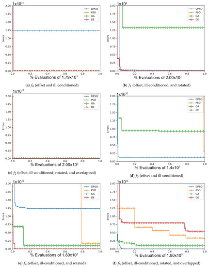
Figure A1.
The average In-Sample (, , ) and Elliptical (, , ) global best results over time for 7 dimensions.
Figure A1.
The average In-Sample (, , ) and Elliptical (, , ) global best results over time for 7 dimensions.
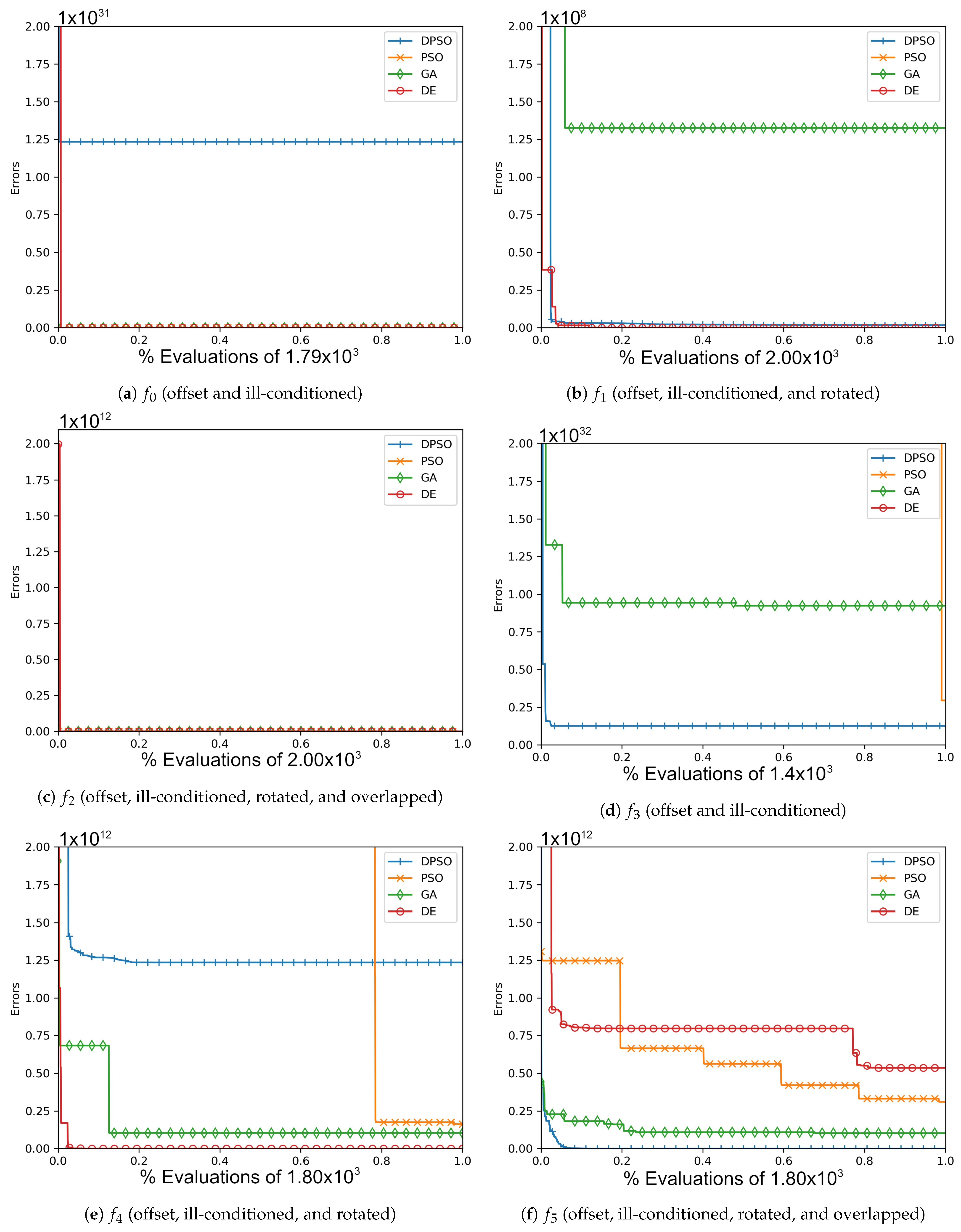
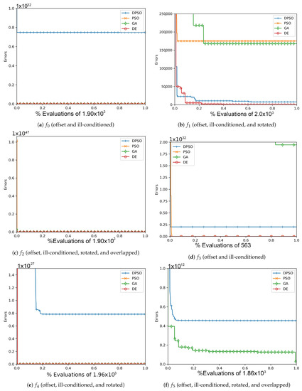
Figure A2.
The average In-Sample (, , ) and Elliptical (, , ) global best results over time for 14 dimensions.
Figure A2.
The average In-Sample (, , ) and Elliptical (, , ) global best results over time for 14 dimensions.
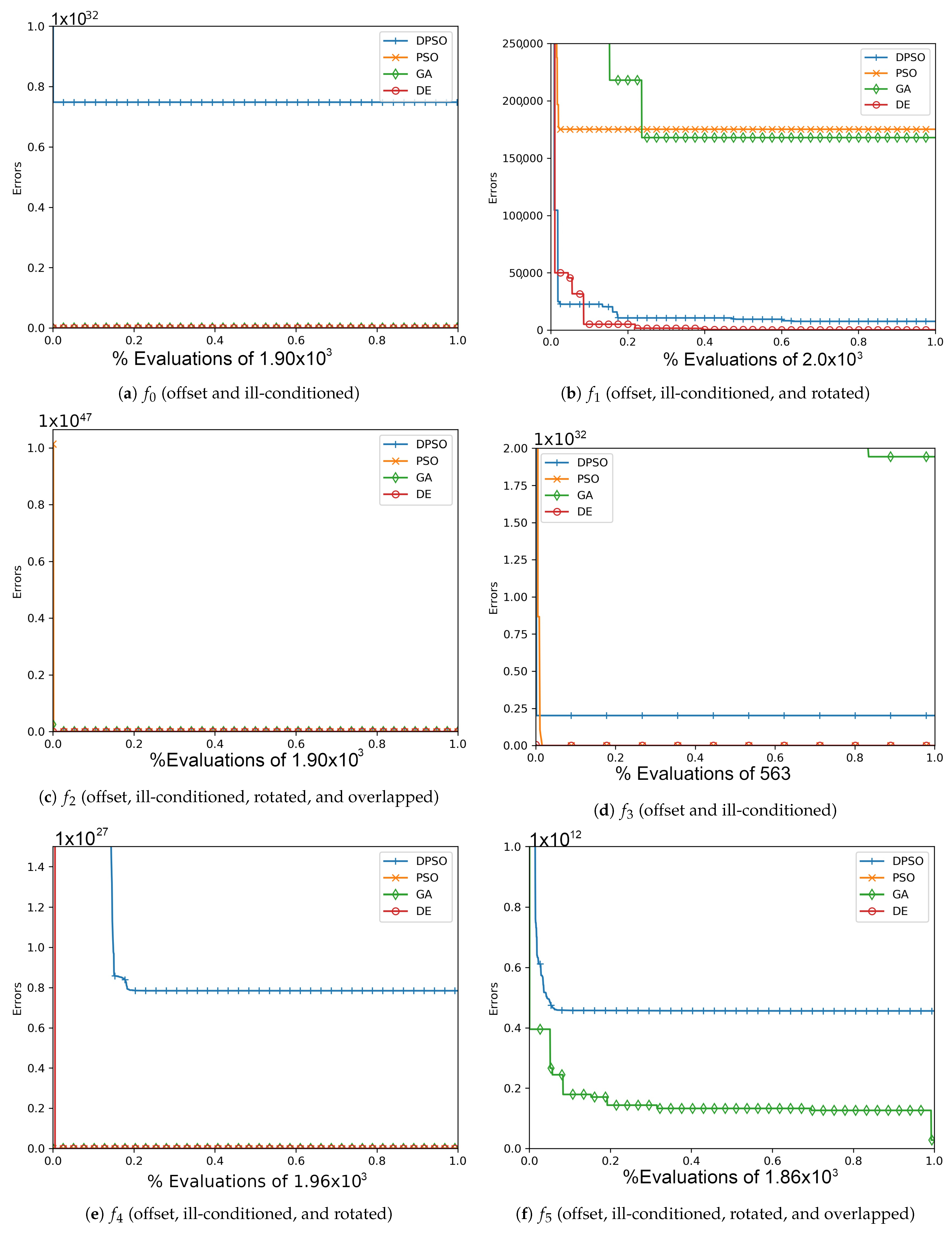
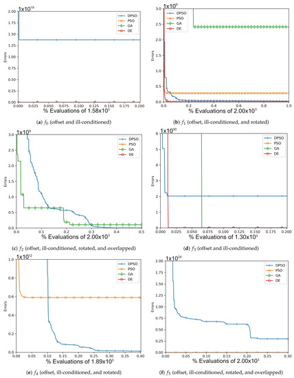
Figure A3.
The average In-Sample (, , ) and Elliptical (, , ) global best results over time for 21 dimensions.
Figure A3.
The average In-Sample (, , ) and Elliptical (, , ) global best results over time for 21 dimensions.
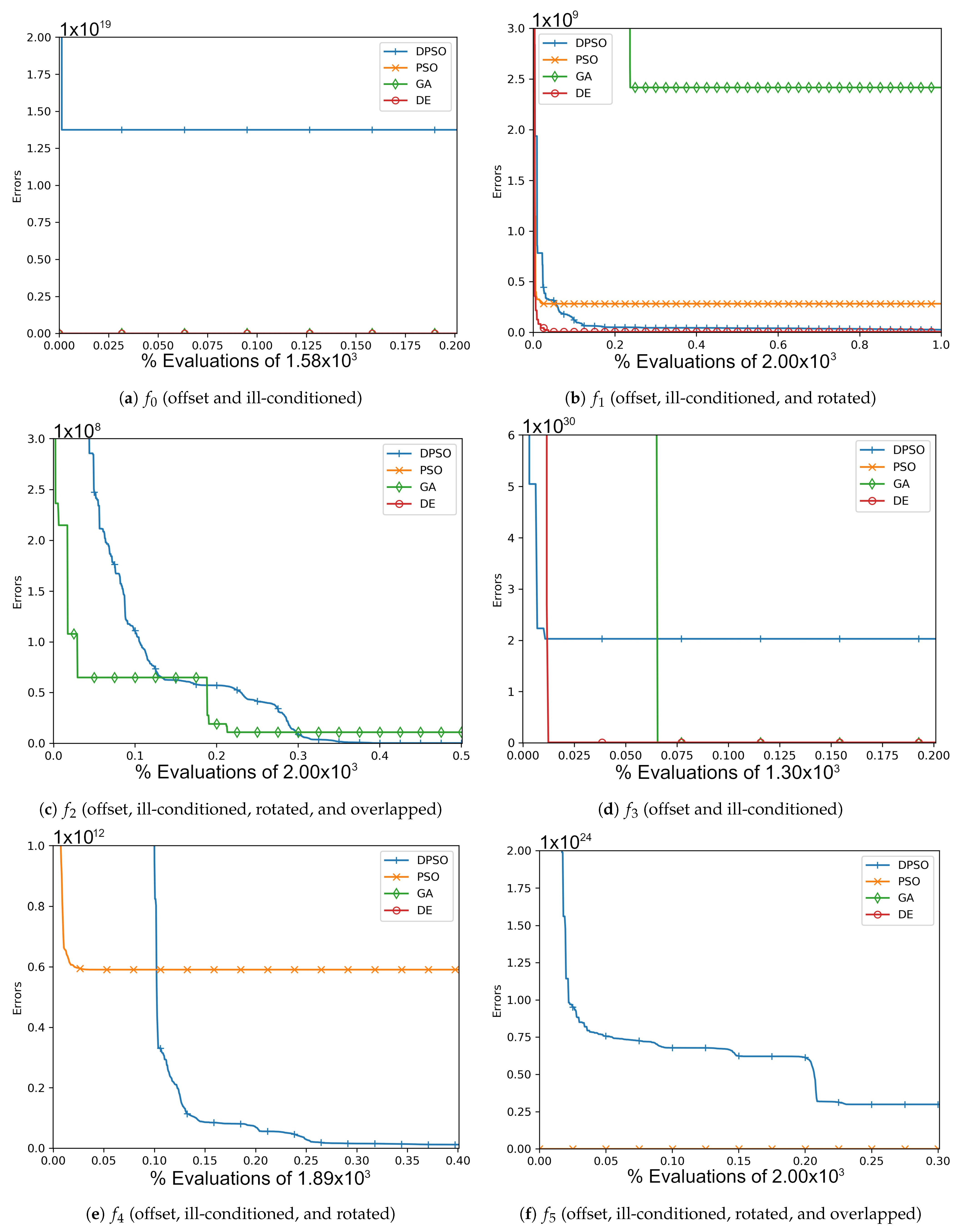
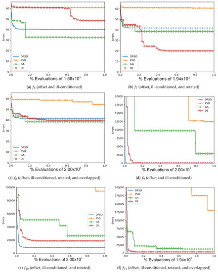
Figure A4.
The average Ackley (, , ) and Rosenbrock (, , ) global best results over time for 7 dimensions.
Figure A4.
The average Ackley (, , ) and Rosenbrock (, , ) global best results over time for 7 dimensions.
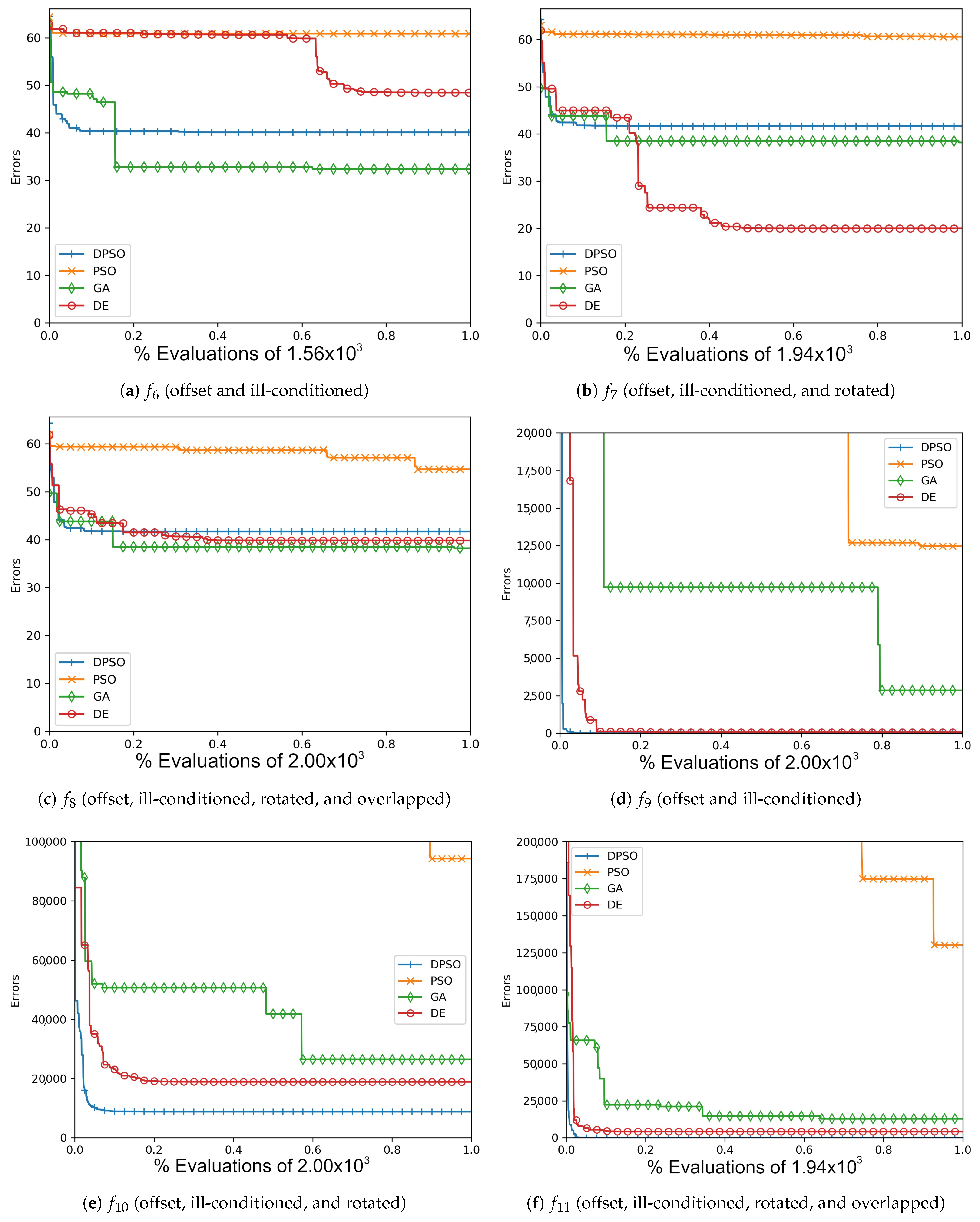
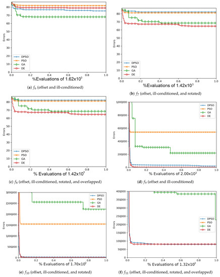
Figure A5.
The average Ackley (, , ) and Rosenbrock (, , ) global best results over time for 14 dimensions.
Figure A5.
The average Ackley (, , ) and Rosenbrock (, , ) global best results over time for 14 dimensions.
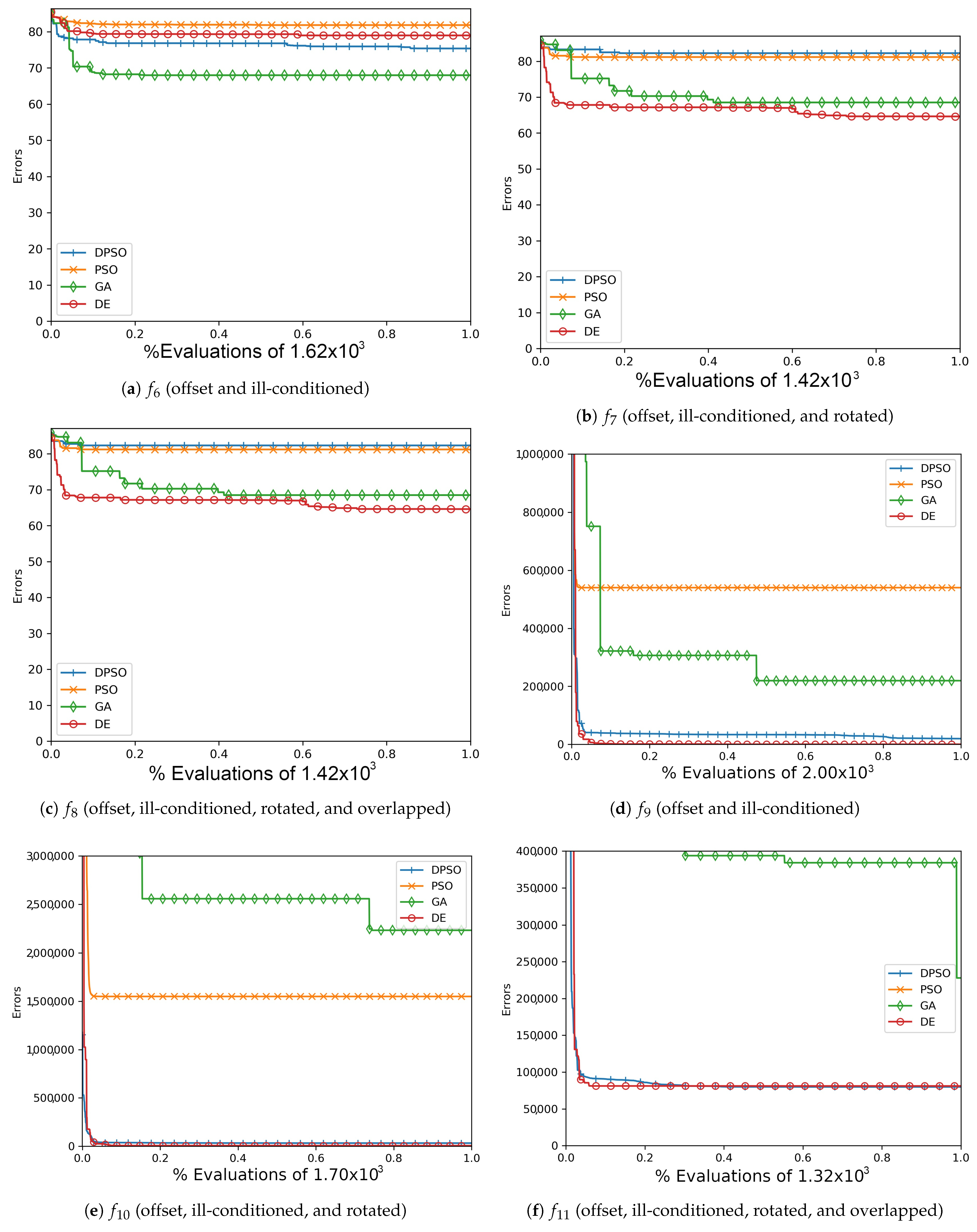
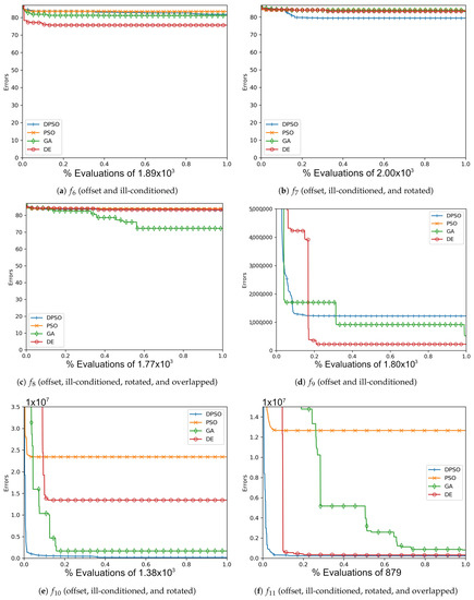
Figure A6.
The averageAckley (, , ) and Rosenbrock (, , ) global best results over time for 21 dimensions.
Figure A6.
The averageAckley (, , ) and Rosenbrock (, , ) global best results over time for 21 dimensions.
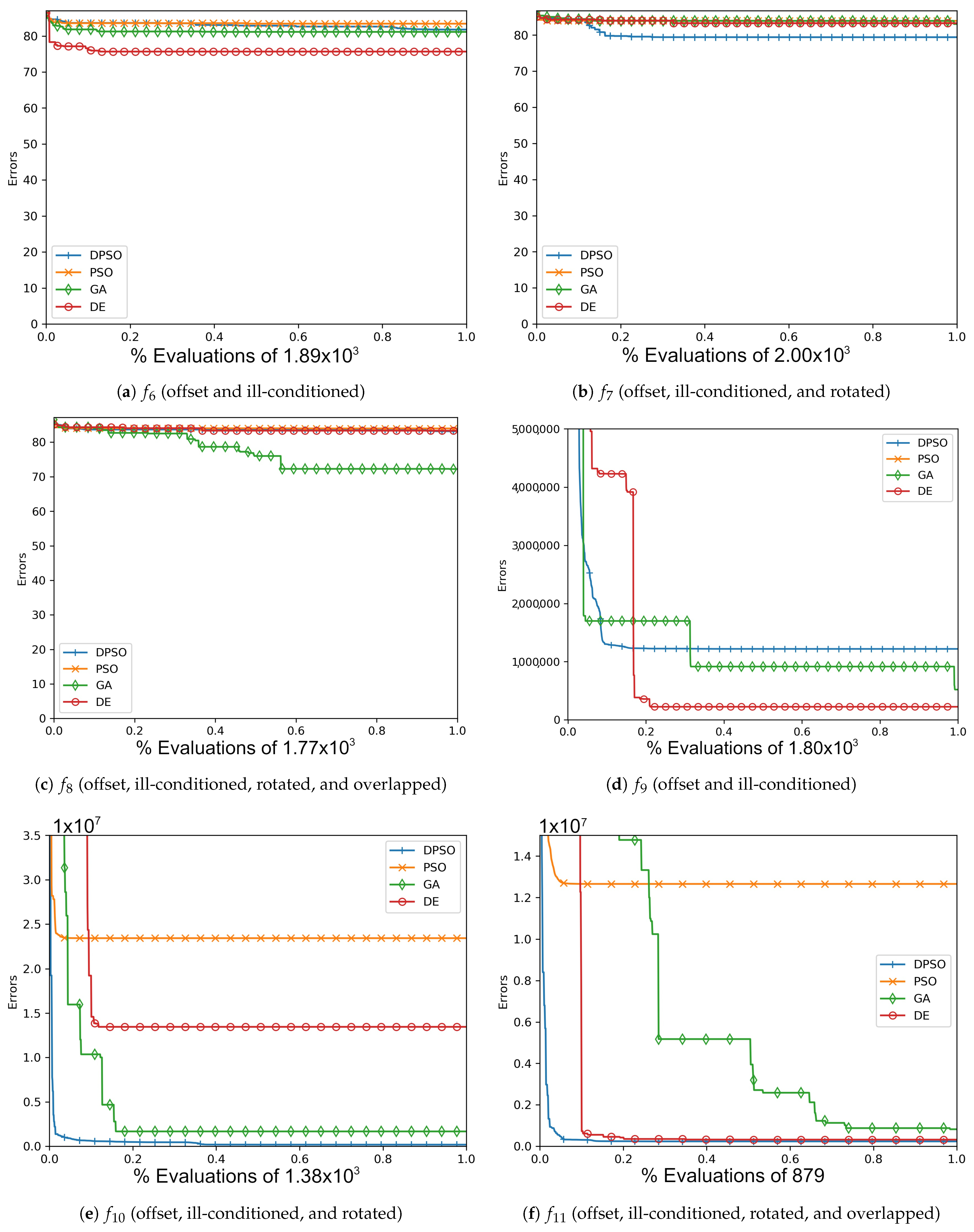
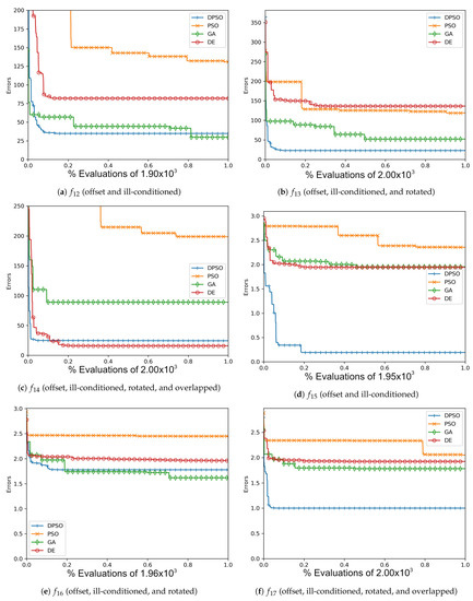
Figure A7.
The average Rastrigin (, , ) and Drop-Wave (, , ) global best results over time for 7 dimensions.
Figure A7.
The average Rastrigin (, , ) and Drop-Wave (, , ) global best results over time for 7 dimensions.
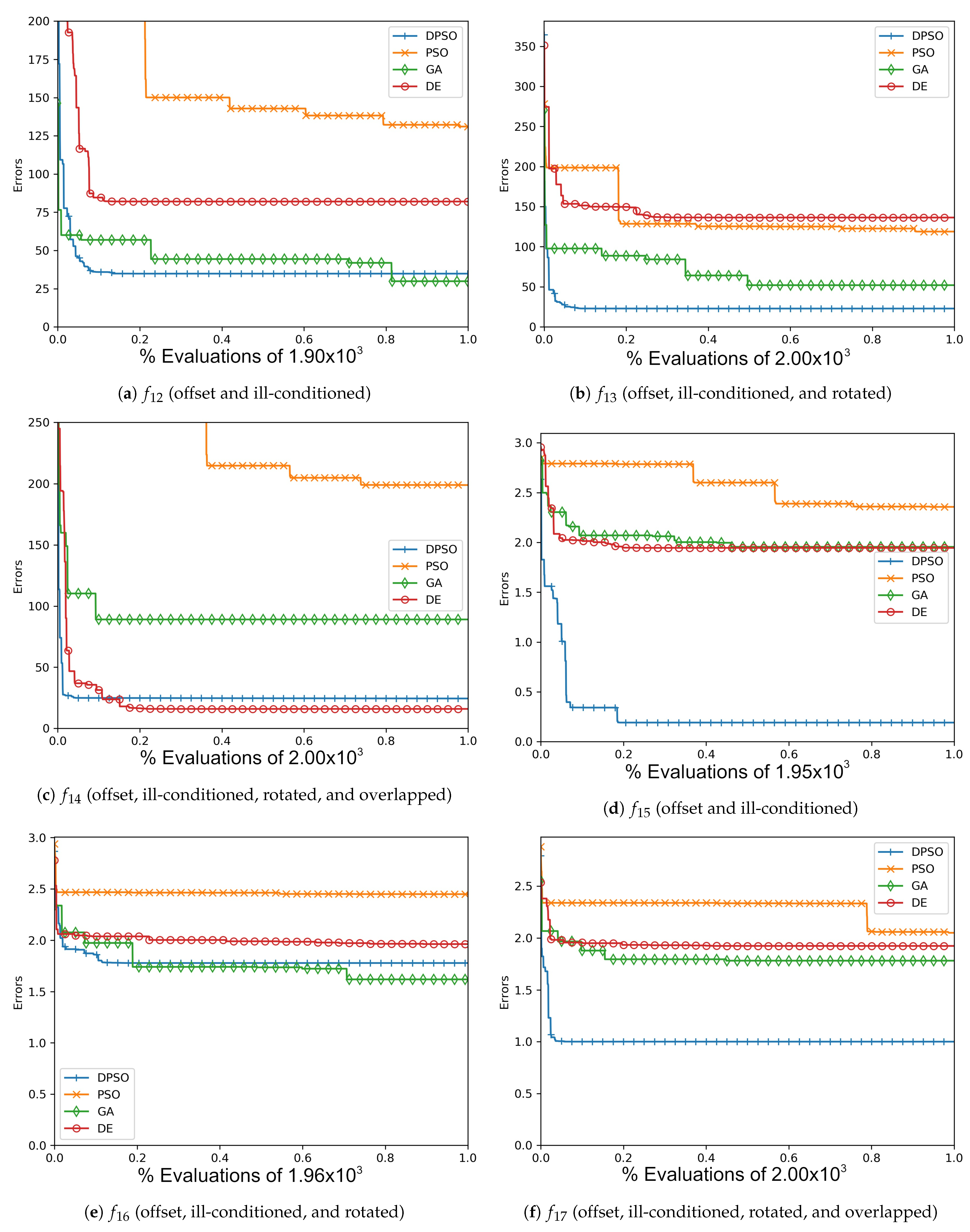
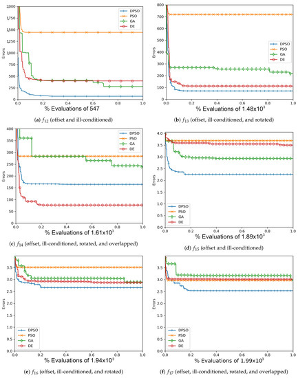
Figure A8.
The average Rastrigin (, , ) and Drop-Wave (, , ) global best results over time for 14 dimensions.
Figure A8.
The average Rastrigin (, , ) and Drop-Wave (, , ) global best results over time for 14 dimensions.
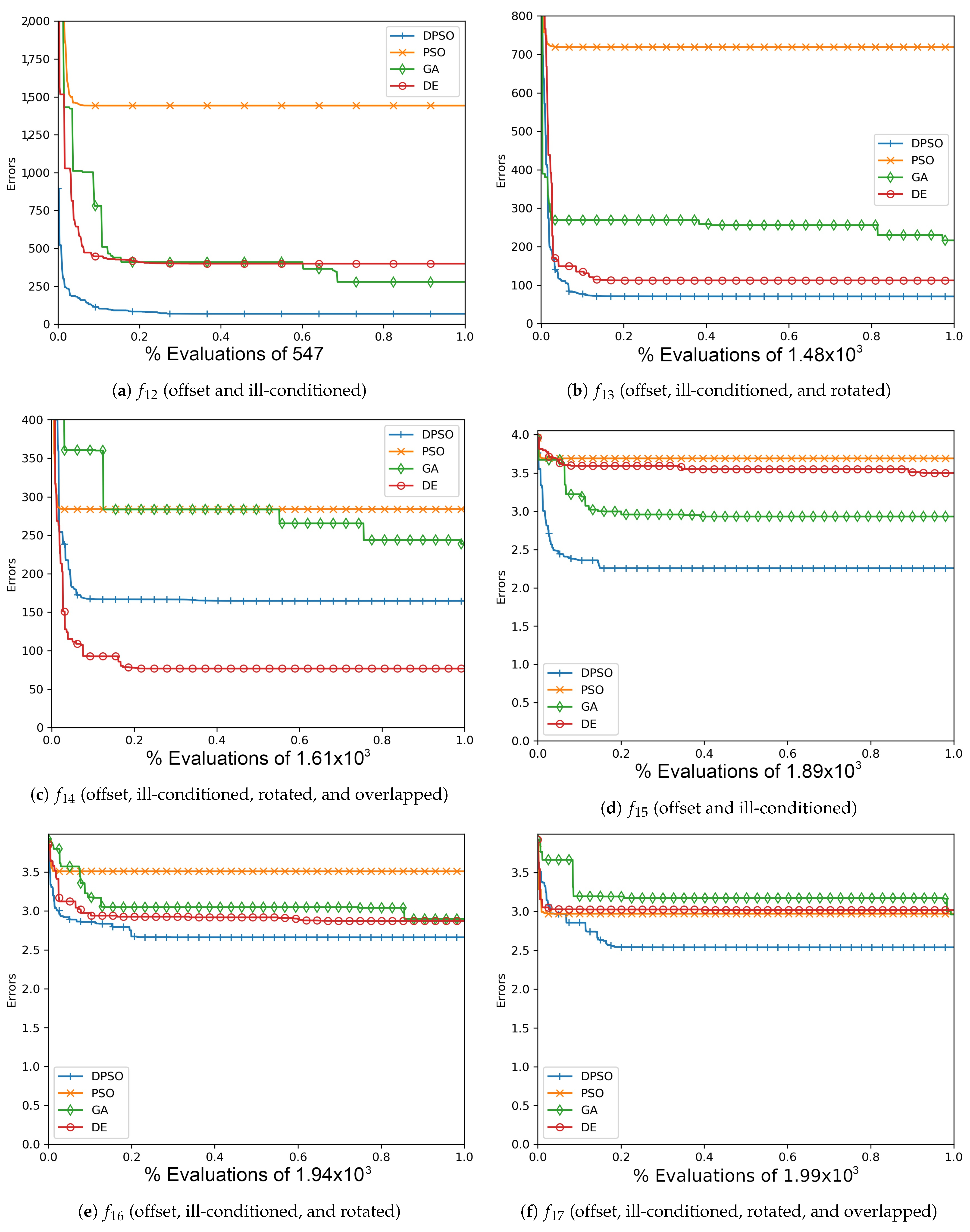
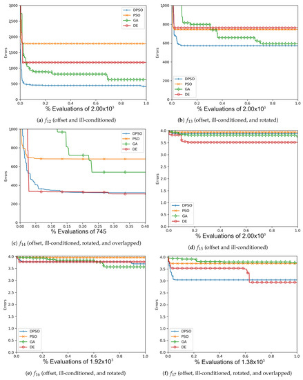
Figure A9.
The average Rastrigin (, , ) and Drop-Wave (, , ) global best results over time for 21 dimensions.
Figure A9.
The average Rastrigin (, , ) and Drop-Wave (, , ) global best results over time for 21 dimensions.
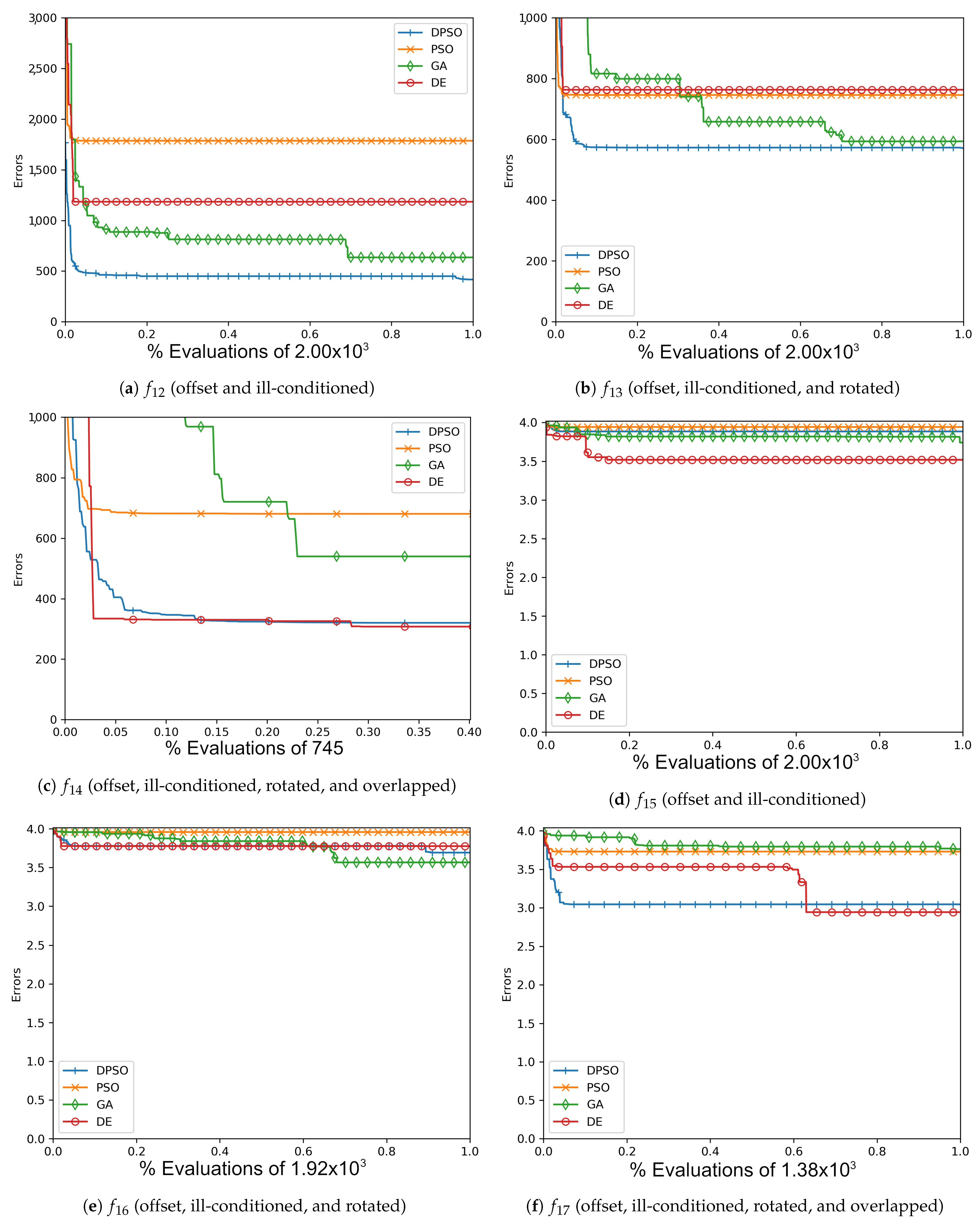
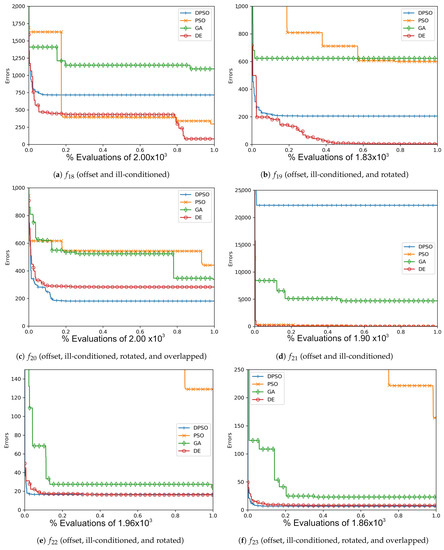
Figure A10.
The averageZero-Sum (, , ) and Salomon (, , ) global best results over time for 7 dimensions.
Figure A10.
The averageZero-Sum (, , ) and Salomon (, , ) global best results over time for 7 dimensions.
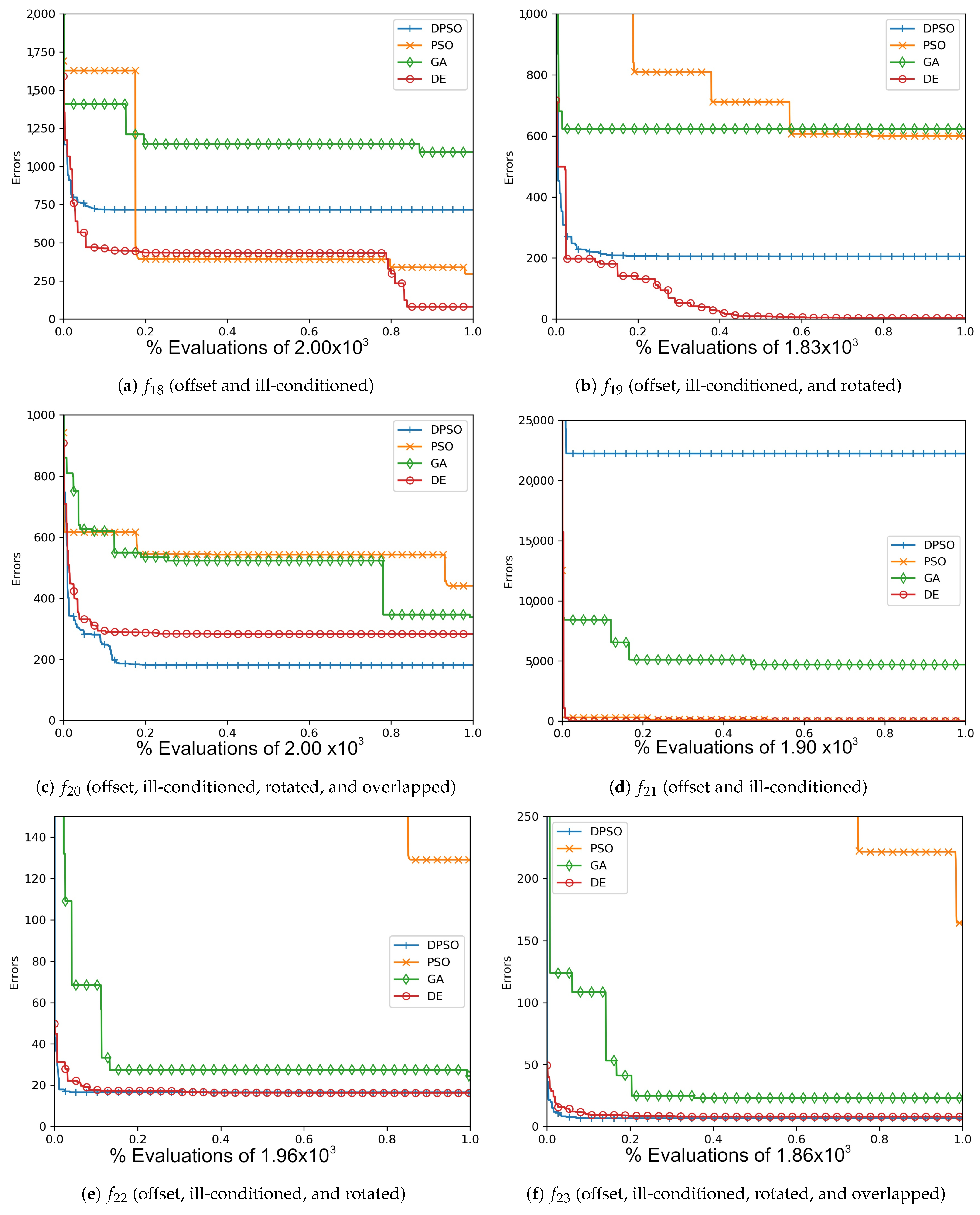

Figure A11.
The average Zero-Sum (, , ) and Salomon (, , ) global best results over time for 14 dimensions.
Figure A11.
The average Zero-Sum (, , ) and Salomon (, , ) global best results over time for 14 dimensions.
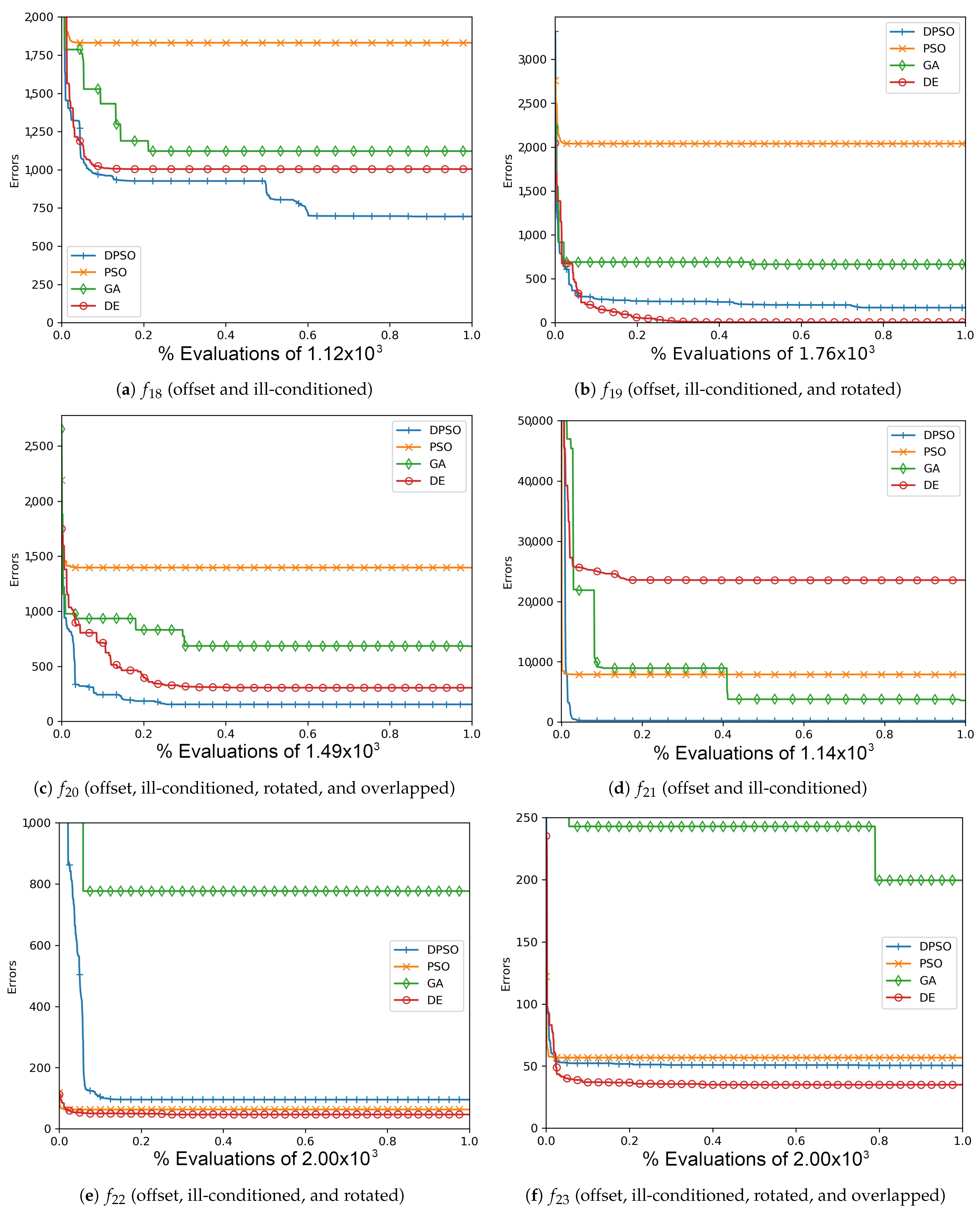
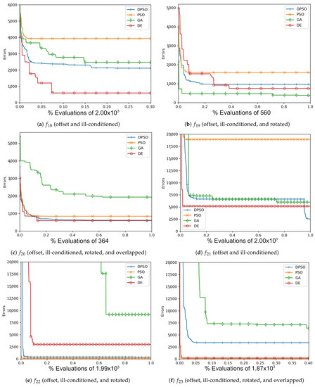
Figure A12.
The averageZero-Sum (, , ) and Salomon (, , ) global best results over time for 21 dimensions.
Figure A12.
The averageZero-Sum (, , ) and Salomon (, , ) global best results over time for 21 dimensions.
References
- Chandrasekar, K.; Ramana, N.V. Performance Comparison of GA, DE, PSO and SA Approaches in Enhancement of Total Transfer Capability using FACTS Devices. J. Electr. Eng. Technol. 2012, 7. [Google Scholar] [CrossRef] [Green Version]
- Deb, A.; Roy, J.S.; Gupta, B. Performance Comparison of Differential Evolution, Particle Swarm Optimization and Genetic Algorithm in the Design of Circularly Polarized Microstrip Antennas. IEEE Trans. Antennas Propag. 2014, 62, 3920–3928. [Google Scholar] [CrossRef]
- Schlauwitz, J.; Musilek, P. A Dimension-Wise Particle Swarm Optimization Algorithm Optimized via Self-Tuning. In Proceedings of the 2020 IEEE Congress on Evolutionary Computation (CEC), Glasgow, UK, 19–24 July 2020; pp. 1–8. [Google Scholar]
- Moodi, M.; Ghazvini, M.; Moodi, H. A hybrid intelligent approach to detect Android Botnet using Smart Self-Adaptive Learning-based PSO-SVM. Knowl.-Based Syst. 2021, 222, 106988. [Google Scholar] [CrossRef]
- Li, B.; Yingli, D.; Penghua, L. Application of improved PSO algorithm in power grid fault diagnosis. In Proceedings of the 2020 Zooming Innovation in Consumer Technologies Conference (ZINC), Novi Sad, Serbia, 26–27 May 2020; pp. 242–247. [Google Scholar]
- Verma, H.; Verma, D.; Tiwari, P.K. A population based hybrid FCM-PSO algorithm for clustering analysis and segmentation of brain image. Expert Syst. Appl. 2021, 167, 114121. [Google Scholar] [CrossRef]
- Lu, G.; Cao, Z. Radiation pattern synthesis with improved high dimension PSO. In Proceedings of the 2017 Progress in Electromagnetics Research Symposium-Fall (PIERS-FALL), Singapore, 19–22 November 2017; pp. 2160–2165. [Google Scholar]
- Zhang, Y.D.; Wu, L. A hybrid TS-PSO optimization algorithm. J. Converg. Inf. Technol. 2011, 6, 169–174. [Google Scholar] [CrossRef]
- Dong, H.; Pan, Y.; Sun, J. High Dimensional Feature Selection Method of Dual Gbest Based on PSO. In Proceedings of the 2020 IEEE Congress on Evolutionary Computation (CEC), Glasgow, UK, 19–24 July 2020; pp. 1–8. [Google Scholar]
- Hichem, H.; Rafik, M.; Mesaaoud, M.T. PSO with crossover operator applied to feature selection problem in classification. Informatica 2018, 42, 189–198. [Google Scholar]
- Molaei, S.; Moazen, H.; Najjar-Ghabel, S.; Farzinvash, L. Particle swarm optimization with an enhanced learning strategy and crossover operator. Knowl.-Based Syst. 2021, 215, 106768. [Google Scholar] [CrossRef]
- Song, S.; Lu, B.; Kong, L.; Cheng, J. A Novel PSO Algorithm Model Based on Population Migration Strategy and its Application. J. Comput. 2011, 6, 280–287. [Google Scholar] [CrossRef]
- Mouna, H.; Mukhil Azhagan, M.S.; Radhika, M.N.; Mekaladevi, V.; Nirmala Devi, M. Velocity Restriction-Based Improvised Particle Swarm Optimization Algorithm. In Progress in Advanced Computing and Intelligent Engineering; Saeed, K., Chaki, N., Pati, B., Bakshi, S., Mohapatra, D.P., Eds.; Springer: Singapore, 2018; pp. 351–360. [Google Scholar]
- Orlando, C.; Ricciardello, A. Analytic solution of the continuous particle swarm optimization problem. Optim. Lett. 2020, 1–11. [Google Scholar] [CrossRef]
- Mousakazemi, S.M.H. Computational effort comparison of genetic algorithm and particle swarm optimization algorithms for the proportional–integral–derivative controller tuning of a pressurized water nuclear reactor. Ann. Nucl. Energy 2020, 136, 107019. [Google Scholar] [CrossRef]
- Abdmouleh, Z.; Gastli, A.; Ben-Brahim, L.; Haouari, M.; Al-Emadi, N. Review of optimization techniques applied for the integration of distributed generation from renewable energy sources. Renew. Energy 2017, 113. [Google Scholar] [CrossRef]
- Hermawanto, D. Genetic Algorithm for Solving Simple Mathematical Equality Problem. arXiv 2017, arXiv:1308.4675. [Google Scholar]
- Eltaeib, T.; Mahmood, A. Differential Evolution: A Survey and Analysis. Appl. Sci. 2018, 8, 1945. [Google Scholar] [CrossRef] [Green Version]
- Sutton, R.S.; Barto, A.G. Reinforcement Learning: An Introduction; Computational Neuroscience Series; MIT Press: London, UK; Cambridge, MA, USA, 2013. [Google Scholar]
- Nobile, M.S.; Cazzaniga, P.; Besozzi, D.; Colombo, R.; Mauri, G.; Pasi, G. Fuzzy Self-Tuning PSO: A settings-free algorithm for global optimization. Swarm Evol. Comput. 2018, 39, 70–85. [Google Scholar] [CrossRef]
- Nobile, M.S.; Pasi, G.; Cazzaniga, P.; Besozzi, D.; Colombo, R.; Mauri, G. Proactive Particles in Swarm Optimization: A self-tuning algorithm based on Fuzzy Logic. In Proceedings of the 2015 IEEE International Conference on Fuzzy Systems (FUZZ-IEEE), Istanbul, Turkey, 2–5 August 2015; pp. 1–8. [Google Scholar]
- Adorio, E.P.; January, R. MVF-Multivariate Test Functions Library in C for Unconstrained Global Optimization; University of the Philippines Diliman: Quezon City, Philippines, 2005. [Google Scholar]
- Gavana, A. Test Functions Index. 2013. Available online: http://infinity77.net/global_optimization/test_functions.html#test-functions-index (accessed on 16 June 2021).
- Li, X.; Tang, K.; Omidvar, M.N.; Yang, Z.; Qin, K. Benchmark Functions for the CEC’2013 Special Session and Competition on Large-Scale Global Optimization. In Proceedings of the IEEE Congress on Evolutionary Computation, Cancun, Mexico, 20–23 June 2013; pp. 1–23. [Google Scholar]


Publisher’s Note: MDPI stays neutral with regard to jurisdictional claims in published maps and institutional affiliations. |
© 2021 by the authors. Licensee MDPI, Basel, Switzerland. This article is an open access article distributed under the terms and conditions of the Creative Commons Attribution (CC BY) license (https://creativecommons.org/licenses/by/4.0/).