Solving the Integrated Multi-Port Stowage Planning and Container Relocation Problems with a Genetic Algorithm and Simulation

Abstract

The greater flow of containers in global supply chains requires ever-increasing productivity at port terminals. The research found in the literature has focused on optimizing specific parts of port operations but has ignored important features, such as the stack-wise organization of containers in a container ship and port yard and the effects of interconnection among the operations in both places. The objective of this paper is to show the importance of designing an integrated plan of the container relocation problem at the port yard with the stowage planning problem for loading and unloading a ship through ports. Both individual problems are NP-Complete, and exact approaches for each problem are only able to find optimal or feasible solutions for small instances. We describe a simulation-optimization methodology that combines simulation, a genetic algorithm, and a new solution representation based on rules. The test results show that the solution from the integrated plan is mutually beneficial for port yards and ship owners.

1. Introduction

Recent container shortage and port congestion scenarios have shown us that maritime port operations can no longer operate as separate fiefdoms but as part of an integrated system. The ship sizes and the global maritime demands continue to increase, demanding properly coordinated operations between ships and ports [1,2].

A port receives containers transported by trucks, trains, and ships. These cargoes are usually temporarily stored in yards and then dispatched. When a ship arrives, there are unloading and loading activities. Several factors influence the port and ship productivity, such as the way the containers are stored in yards, the sequence in which they are removed from stacks, the scheduling of vehicles to transport them to the loading area, the number of quay cranes used, their operation to load the cargo into the vessel, and the way the containers are positioned on the ship. Most of these steps require a complex decision process, which is a common and accepted practice in port operations, and the related literature to treat these tasks separately and sequentially.

In the maritime transport of containers, the ships usually have a circular route, spending a long time at ports [3]. The multi-port stowage planning problem (MPSP) consists of determining how to stow a given set of containers of different types into a set of available locations on a container ship [4,5]. The containers may have different port destinations. The containers are stored in stacks so they can be removed only by the top. If a given container must be unloaded in a port, but it is not on the top, then the containers above it must be removed first. This movement is called reshuffling, and it must be minimized to improve port efficiency. To avoid such inconvenience, it is necessary to elaborate on a suitable stowage plan.

Meanwhile, in the port yard, due to space constraints, yard containers are also organized in stacks. Given this, the container relocation problem (CRP) seeks an optimal operation plan that leads into a retrieval sequence with the fewest relocations to save time and money.

However, the multi-port stowage planning problem (MPSP) impacts the container relocation problem (CRP) [6] for all port yards visited along a ship’s route, requiring an integrated plan of both problems to achieve better quality solutions for the shipowner and all the container terminals along the ship’s route [1,7].

Nevertheless, there are two alternatives to solve the integrated planning binary model: a sequential resolution of mathematical models or solving one monolithic mathematical model [8,9]. Both approaches suffer from an increase in the number of binary variables and constraints that makes them impractical to obtain in an affordable time even feasible solutions.

Therefore, an alternative to overcome such a difficulty is to apply heuristic approaches to solve this integrated problem. The genetic algorithm has been one interesting technique to solve combinatorial decision-making problems, because it obtains quality solutions with a reasonable computation time. In particular, this paper adapts an approach used for the joint problem of multi-port stowage planning and quay crane scheduling [9].

The paper’s contributions are the following:

1.

We show the importance of developing an integrated plan for the MPSP and CRP problems to provide a better solution than the one obtained by performing isolated or simplified plans, as reported in the literature.

2.

We extend the methodology employed for the MPSP in a manner that enables a fast solution to the MPSP and CRP, thus avoiding the high computational burden required by the exact approaches to solving such large-scale problems.

3.

Our approach guarantees that the multi-port stowage plan obtained is executable by the port terminal and the sequence of retrieved containers from the yard is also good for the ship, thereby making the solution advantageous for all port terminals and the shipping company by reducing the total number of container movements.

This paper is organized as follows. Section 1 gives a detailed description of the problems. Section 2 presents the modeling of the integrated problem. Section 3 explains the methodology used. Section 4 presents and discusses the results obtained, and Section 5 presents the conclusions and future work.

Related Works

When the ship comes to the port, initially the containers destined for the port are unloaded, and then a set of containers at the yard is retrieved from the stacks and loaded into the vessel through quay crane operations. These retrievals from the yard stacks constitute a combinatorial problem [10]. The quay crane operation also must attend to some specific operational constraints, such as quay crane non-crossing, non-overtaking, and safety distance constraints [11]. These approaches consider each problem separately.

More recently, many models integrated some of these problems. For example, the operation of a yard crane, the scheduling of yard vehicles, and loading operations executed by a quay crane are modeled jointly in [12,13,14]. In [15,16], the issue of yard location assignment problems is integrated with the interaction of a yard transport vehicle, while ref. [17] integrated the yard location assignment with the dispatching of yard crane units. Ref. [18] jointly treated the quay crane assignment problem with the problem of storage space assignment. In [19], the problem of the yard transport vehicle routing was integrated with quay crane and yard crane operations. Facing similar problems, ref. [20] integrated two different railroad container terminals problems and emphasized the positive impact of establishing decision support tools for solving interdependent problems in an integrated manner. Simulation-based approaches were also present in [21] to solve the problem of railway traffic flow.

In the ship, the container assignment must take into account the locations for specific container types and other requirements such as vessel stability, height, and weight limits. The position of the container on the stacks must also consider its destination to avoid reshuffle operations in future ports. This is also a combinatorial problem, and commonly, a hierarchical approach is used, in which the liner shipper establishes a master plan, also called the master bay planning problem (MBPP), and the port terminal determines a sequence of cargo loading and the cargoes’ positions on the ship [22,23].

There are not many papers that investigate multi-port stowage planning. The first model was proposed in [24], and after that, several papers were presented [3,5,25,26,27,28,29,30,31]. The methods adopted by these papers can be grouped into three classes: (1) a single mathematical model, (2) hierarchical planning, and (3) heuristic models. In the class of the single mathematical model, multi-port stowage planning is formulated as a unique optimization problem [5,24]. Although mathematically elegant, these single models use a simplified representation of the ship with a single bay and all containers being the same size, creating difficulty in treating realistic size problems. To overcome these difficulties, there are hierarchical models. They use decomposition in the master planning and container allocation sub-problems [3,25,28,29,30]. Other models use only heuristics, as in [3,26,27].

Some papers, such as [31,32], have taken into account some characteristics of the containers, such as the dimensions (e.g., standard, 45-footer, high-cube, or oversized), weight class (light, medium, or heavy), type (reefer or open-top), load (dangerous or perishable), and port of destination. Despite that, these papers focus on the export flow at the one-port ship loading problem, ignoring the cargo arrangement in yard stacks. Here, we integrate the entire flow of the containers between the port yards and the ship.

Ref. [27] presented two genetic algorithm (GA) approaches to multi-port stowage planning. In the first one, the dimension of the chromosome was equal to the number of cells of the ship. A realistic problem results in a very large vector, which makes the GA search very inefficient. A second representation was proposed called compact encoding, in which only the unloading and loading containers were represented. The representation of the chromosome adopted in this paper has some similarity to the compact encoding, since the unloading and loading containers are represented.

A GA was also used in [33] to study the CRP under multiple quay crane parallel operations. Three strategies were presented to minimize the number of rehandles: the nearest stack strategy, the lowest stack strategy, and the optimization strategy. The last one consists of selecting the stack which does not contain the next loading container to relocate the obstructing container. The GA was designed to apply these strategies. The container classes were not considered, and the authors assumed that the containers were all the same size within a bay. Instances of up to 980 containers were tested.

The next section details the modeling of the problem.

2. Modeling the Problem

In our problem, the journey of P ports of a ship is represented. In each port $p=1,\dots ,P-1$, where this ship docks, there is a yard with containers that must be loaded onto it. At the first port, $p=1$, the ship arrives empty and receives the loading of the containers that were at the yard of this port, as illustrated in Figure 1.

At ports $p=2,\dots ,P-1$, the ship first unloads the containers destined for port p, where it currently is (see Figure 2), and then receives the loading of containers destined for the following ports (see Figure 3). Finally, when the ship arrives at the last port of its journey P, only the unloading is performed.

Observe that the numbers on the containers identify each container, and when at the port yard, this represents the removal order, starting with the smallest number and ending with the largest number contained in each yard. This order comes from a previous solution of the stowage plan, as is the convention for the CRP. Regarding removal from the ship, a dictionary contains the destination port of each container, and it must be consulted to find out which containers should be unloaded at which ports.

In Figure 2, note that the ship arrives at the second port of its route, and it has to unload the four highlighted containers (3, 6, 11, and 14), of which two of them are not at the top of their stacks. For this reason, first, the blocking container (number 9) located above containers 6 and 3 will be unloaded to a reserved area of the yard, which is not the same area of the import containers nor the export containers, which are about to be loaded. Next, it can be seen in Figure 3 that after all containers destined for this port are unloaded from the ship, the container loading operation at the second port yard with the relocated containers starts. The rules proposed follow this representation and are described in detail in the following section.

The following assumptions have been made based on [24,34] for the sake of simplicity without compromising the general application of the solutions:

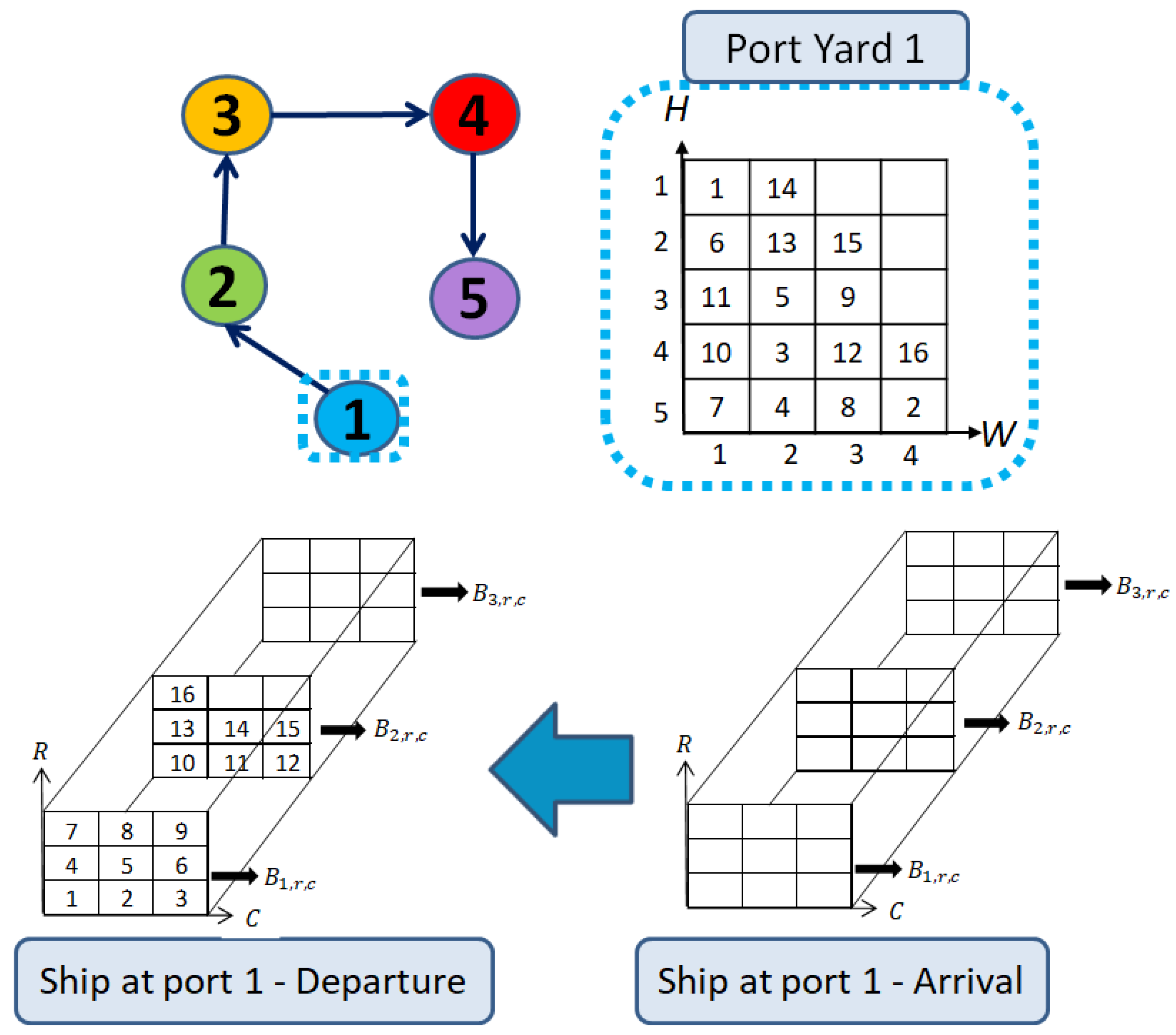
• The container ship has a rectangular format and can be represented as a matrix, called the ship’s occupation matrix ($Shp$), with rows ($r=1,2,\dots ,R$), columns ($c=1,2,\dots ,C$), and bays ($b=1,2,\dots ,B$) and a maximum capacity of $R\times C\times B$ containers. Each space to store a container is a coordinate ($r,c,b$), where $r\in R$, $c\in C$, and $b\in B$. An irregular format may be achieved by simply adding constraints that represent imaginary containers that occupy the same spaces during the whole voyage [26].
• The yard can also be represented as a matrix called $yar{d}_p$, with rows ($i=1,\dots ,H$) and stacks ($j=1,\dots ,W$). Each space to store a container is a coordinate ($i,j$), where $i\in H$ and $j\in W$.
• All containers have the same size and weight and are accessible only from the top.
• All containers in the port yard will be loaded onto the ship.
• The container ship can always carry all the containers at each port p, and its capacity will never be exceeded.
• In each yard, there must be at least $H-1$ empty positions to guarantee the accessibility of any container. Analogously, onboard the ship, there must be at least $R-1$ empty positions to guarantee the accessibility of any container.
• The unloaded containers are destined for a specific area of the port yard and are not mixed with the containers that are going to be loaded nor with the relocated containers, as illustrated in Figure 2 and Figure 3.

Note that the assumptions made about the containers’ weight and size are not a limitation of the representation, since it enables a focused analysis on how ship and yard container arrangements are affected by integrated planning.

Given these points, we can now introduce the constraints that the simulation optimization must respect:

• Each position $(i,j)$ in the yard and $(r,c,b)$ on the ship must be occupied by at most one container.
• No “holes” are allowed in the stacking area, meaning that if there is a container in position $(i,j+1)$, then the lower position $(i,j)$ must also be occupied. Likewise, if there is a container is in position $(r,c+1,b)$ on the ship, then the lower position $(r,c,b)$ must also be occupied.
• The last in, first out (LIFO) policy must be respected, meaning that if container n is below container q, then container n must be moved before container q.
• No container can be relocated to a position in the same column.
• In the yard, a container in position $(i,j)$ can only be moved if the position $(i,j+1)$ above it is empty. Likewise, on the ship, a container in position $(r,c,b)$ can only be moved if the position $(r,c+1,b)$ above it is empty.
• The containers are removed from the yard one at a time and then loaded onto the ship.
• Container n, after being loaded onto the ship, does not change its position while the ship is still stopped at the same port.
• When a container is unloaded and loaded back onto the ship, these operations are counted as one relocation movement.
• The containers relocated outside the ship are always loaded back onto it before the export containers at the port yard.

Any readers interested in the mathematical formulation of these constraints can reefer to [35]. In the next section, the methodology used here is described in detail.

3. Methodology

Our methodology deals with both the CRP and MPSP concomitantly, aiming to reduce the total number of relocations for both the yards and the ship. This way, it is possible to ensure an efficient operation between the ship and port.

The assumptions presented in the previous section were represented through the simulation modeling that is detailed in Algorithm 1. To define how exactly the loading and unloading would occur, rules representation was used. The rules are functions containing logical commands that describe actions that result in the movement of containers. This means that instead of creating binary variables and corresponding equations that control the position of each container in the ship or the yard, we created generic procedures for how to retrieve and reshuffle containers in the yard and unload and load containers out of and onto the ship.

The rules that define the plan for the ship stowage operations and the port yard were coded in one vector and passed to the simulation program as a parameter. This parameter was an individual of the genetic algorithm (GA) and represented a possible solution to the problem. After simulating the rules represented by a certain individual, we had the total number of relocation movements performed, which was going to be used by the GA to calculate the fitness value of this individual.

The mapping through rules representation was already successfully applied to isolated or specific integrated port operations: the multi-port stowage planning problem [36], multi-port stowage planning integrated with quay crane operation [9], or even multi-port stowage planning with the container relocation problem [35].

The GA generated and selected various individuals in such a way that the total number of relocations performed was minimized, which was the objective of our problem. In the end, the GA would provide the combination of rules that solved each instance of the problem with the least number of relocation movements.

The use of a method based on rules is justified since it is necessary to provide a feasible solution in a small amount of time for the decision maker. This is not possible even for solving the problems separately when using exact models, as can be seen in [35]. Additionally, our method always produces feasible occupation matrices, facilitating and ensuring the achievement of feasible solutions by heuristic methods.

The main advantage of this methodology is that there is no limit to the number of rules that can be incorporated. The rules can be simple, sophisticated, or even take into account different operator practices or the prior knowledge of skilled personnel. Any rule can be created, simulated, and have its solution evaluated by the genetic algorithm.

In the literature, there is a specific term for approaches that limit the search space in terms of easy-to-implement low-level heuristics: hyper-heuristic methods [37,38].

Additionally, heuristics are general enough to be applied to several instances of the same problem class, enabling uncertainty evaluation through the evaluation of multiple scenarios [39].

It is important to stress that the literature considers hyper-heuristics as a heuristic to select one combination of heuristics [37]. Since we employed a meta-heuristic, such as a genetic algorithm, to select a good quality combination of rules, we classified our approach as a meta-hyper-heuristic approach.

Taking this into account, first, we will individually explain each rule proposed to solve the CRP, followed by the rules proposed for the MPSP. Then, we will explain the integration of both problems by using the simulation program and the search for the best solution using the genetic algorithm.

3.1. Rules Representation for the CRP

To represent the flow of containers through a port yard, an occupation matrix $yar{d}_p$, where $p=1,2,\dots ,P$, was employed as illustrated in Figure 1. In each position (i,j), where $i\in H$ and $j\in W$, there is an index representing a container. As stated, this index represents the removal order of the containers; that is, container 1 is the first one to be retrieved, followed by container 2, and so on until container $N_p$.

For all rules, if the target container is at the top of its stack, and it is retrieved from the yard. Otherwise, an available position within the yard’s stacking area must be found to relocate it and clear the access to the target container. To do so, the retrieval rules ($R{r}_e$) run a search through the yard in a fixed pattern, which is different for each rule. When the available position is located, the first blocking container is relocated to this position. This procedure is repeated for all blocking containers above the target container. This step is completed when all containers from the yard are retrieved.

All the $R{r}_e$ rules necessary for this operation will now be described in detail. The first four $R{r}_e$ rules are adaptations of the rules presented in [40]. Rules $R{r}_5$ and $R{r}_6$ are unpublished in the literature. The last four rules were proposed in the literature and properly adapted to be included in our solution method: the $R{r}_7$ rule was proposed in [34], $R{r}_8$ in [41], and $R{r}_9$ and $R{r}_{10}$ in [33]:

• Rule $R{r}_1$: To locate an available position, this rule searches the yard’s occupancy matrix in a fixed direction, starting from the last row H to the first row $h=1$, row by row, and from left to right; that is, the stacks are arranged such that $w=(1,2,\dots ,W)$, as illustrated in Figure 4a.
• Rule $R{r}_2$: To locate an available position, this rule searches the yard’s occupancy matrix in a fixed direction, starting from the last row to the first row, stack by stack, and from left to right, as illustrated in Figure 4b.
• Rule $R{r}_3$: This rule reverses the direction used in rule $R{r}_1$. To locate an available position, it searches the yard’s occupancy matrix in a fixed direction, starting from the last row to the first row, row by row, and from right to left; that is, the stacks are arranged such that $w=(W,W-1,W-2,\dots ,1)$, as illustrated in Figure 4c.
• Rule $R{r}_4$: This rule reverses the direction used in rule $R{r}_2$. To locate an available position, it searches the yard’s occupancy matrix in a fixed direction, starting from the last row to the first row, stack by stack, and from right to left as illustrated in Figure 4d.
• Rule $R{r}_5$: To locate an available position, this rule searches the yard’s occupancy matrix in a fixed direction, starting from the last row to the first row, row by row, and alternating the direction in each row; that is, the last row H goes from left to right, row $H-1$ goes from right to left, and so on until row $h=1$, as illustrated in Figure 4e.
• Rule $R{r}_6$: This rule is the reverse of rule $R{r}_5$. To locate an available position, it searches the yard’s occupancy matrix in a fixed direction, starting from the last row to the first row, row by row, and alternating the direction in each row; that is, the last row H goes from right to left, row $H-1$ goes from left to right, and so on until row $h=1$, as illustrated in Figure 4f.
• Rule $R{r}_7$: To relocate the blocking containers, this rule performs a computation of a stack score based on the removal priority of the containers at the yard. The goal is to relocate the blocking container to a new position where there are no containers that are going to be retrieved before it. If there is no such position available, then the stack chosen is the one that has the latest future relocation. For more details, see [34].
• Rule $R{r}_8$: This rule is similar to rule $R{r}_7$, but it allows one “cleaning move” under certain conditions when identifying eligible positions to relocate a blocking container. This means that a container that is not in the same stack as the target container can be moved to make room for a blocking container to avoid future relocation. In Figure 5, note that when the highlighted container 1 will be retrieved, if container 2 had not been first relocated to position $(4,1)$, at least two more relocations would have had to be executed to retrieve all containers from the yard. For more details, see [41].
• Rule $R{r}_9$: This rule chooses the lowest stack that has an available position to relocate the blocking container. In the case of multiple stacks with the same lowest height, the nearest one is chosen. For more details, see [33].
• Rule $R{r}_{10}$: This rule chooses the nearest stack that has an available position to relocate the blocking containers. For more details, see [33].

The next section describes the loading ($L{r}_l$) and unloading ($U{r}_u$) rules for the stowage planning problem.

3.2. Representation by Rules for the MPSP

The containers are loaded onto the ship one-by-one as they are being retrieved from the yard, which means that it is the $R{r}_e$ rule that calls the $L{r}_l$ rule each time one container is retrieved from the yard. Thus, the $L{r}_l$ rules aim to find a position on the ship to put the container that is being loaded.

As illustrated in Figure 1, each position $(r,c,b)$ of the ship matrix can store a container, which is represented by an index. A dictionary contains the information of the destination port of each container, and it is used by some of the $L{r}_l$ rules and for all $U{r}_a$ rules. Most of the $L{r}_l$ rules scan the ship matrix in a fixed direction, and when the first available position is found, the container is loaded onto that position. This step is completed when all containers from the yard have been loaded onto the ship.

Next, all the $L{r}_l$ rules are described in detail. The rules were initially proposed in [36,42] and have been adapted for the loading operation described:

• Rule $L{r}_1$: To locate an available position for the container that is being loaded, this rule searches the ship’s occupancy matrix in a fixed direction, starting from the last row R to the first row $r=1$, row by row, and from left to right; that is, the stacks are arranged such that $c=(1,2,\dots ,C)$ for each bay at a time, starting from bay $b=1$ to bay $b=B$, as illustrated in Figure 6a.
• Rule $L{r}_2$: To locate an available position, this rule searches the ship’s occupancy matrix in a fixed direction, starting from the last row R to the first row $r=1$, stack by stack, from left to right, and from bay $b=1$ to bay $b=B$, as illustrated in Figure 6b.
• Rule $L{r}_3$: This rule reverses the direction used in $L{r}_1$. It searches the ship’s occupancy matrix starting from the last row R to the first row $r=1$, row by row, and from right to left; that is, the stacks are arranged such that $c=(C,C-1,C-2,\dots ,1)$ from bay $b=1$ to bay $b=B$, as illustrated in Figure 6c.
• Rule $L{r}_4$: This rule reverses the direction used in $L{r}_2$. It searches the ship’s occupancy matrix starting from the last row R to the first row $R=1$, stack by stack, and from right to left; that is, the stacks are arranged such that $c=(C,C-1,C-2,\dots ,1)$ from bay $b=1$ to bay $b=B$, as illustrated in Figure 6d.
• Rule $L{r}_5$: To locate an available position for the container that is being loaded, this rule searches the ship’s occupancy matrix in a fixed direction, starting from the first row $r=1$ to row R and filling up the ship by row but interleaving the bays (i.e., from bay $b=1$ to $b=B$), as illustrated in Figure 7a.
• Rule $L{r}_6$: To locate an available position for the container that is being loaded, this rule searches the ship’s occupancy matrix in a fixed direction, starting from the first row $r=1$ and interleaving the bays (i.e., from bay $b=1$ to $b=B$, filling up by stack, and starting from stack $c=1$ to stack $c=C$), as illustrated in Figure 7b.
• Rule $L{r}_7$: This rule reverses the direction used in $L{r}_5$. It searches the ship’s occupancy matrix starting from the last row R to row $r=1$, filling up the ship by row but interleaving the bays (i.e., from bay $b=1$ to $b=B$), as illustrated in Figure 7c.
• Rule $L{r}_8$: This rule reverses the direction used in $L{r}_6$. It searches the ship’s occupancy matrix starting from the last row R to the first row $r=1$, filling up the ship by stack but interleaving the bays (i.e., from bay $b=1$ to $b=B$), as illustrated in Figure 7d.
• Rule $L{r}_9$: This rule fills the ship by bay from bay $b=1$ to bay $b=B$, and at each bay, it uses a stack score based on the removal priority of the containers in the yard to choose a position to allocate the incoming container, similar to what was performed to choose a position for a blocking container in rule $R{r}_7$. It seeks to put in the same stack containers that are going to be unloaded at the same or previous port, putting at the bottom the containers with the furthest destination port. If a container is being loaded, and all stacks already have containers that are going to be unloaded before it, the rule chooses the stacks that lead to the most distant relocation. For example, if there are three stacks available, and the first container to be unloaded at each stack is for port 3, port 4, and port 5, then the rule will choose the port 5 stack.
• Rule $L{r}_{10}$: This rule is the same as rule $L{r}_9$, with the difference that when there is no stack to allocate a container where it will not cause any further relocation, it chooses the stack with the nearest relocation. For example, if there are three stacks available, and the first container to be unloaded at each stack is for port 3, port 4, and port 5, then the rule will choose the port 3 stack.
• Rule $L{r}_{11}$: This rule fills the ship by bay from bay $b=1$ to bay $b=B$, choosing the smallest stack to relocate a container. If there are multiple columns with the same height, then it chooses the leftmost stack (i.e., from stack $c=1$ to $c=C$).

Finally, to unload the containers from the ship, the unloading rules $U{r}_a$ are used. This step is completed when all containers from the ship destined for port p have been unloaded:

• Rule $U{r}_1$: At any port p, this rule will only remove the containers whose destination is port p and all the ones that are blocking the stacks.
• Rule $U{r}_2$: This rule states that all containers on the ship must be unloaded when arriving at a specific port p to allow for a complete rearrangement of every stack.
• Rule $U{r}_3$: This rule was adapted from [43] and allows a blocking container to be internally relocated by repositioning it from one position in the ship bay b to another position in the same ship bay b if there is space to relocate it in this bay b and when it does not cause a future relocation; that is, in this stack, there are no containers that are going to be unloaded before the relocated container. Otherwise, it is unloaded from the ship.

All containers that were unloaded from the ship at a port that was not their destination are loaded back after the unloading operation is finished by using the $R{r}_e$ and $L{r}_l$ rules that were at the gene applied to that port.

Now, we will show how these ship and yard rules may be integrated for use in the simulation program.

3.3. Integrating the Rules for the MPSP and CRP

For the rules to be used by the simulation program, they needed to be combined into a set of decision rules called $R{e}_j$.

Therefore, we had 10 rules for yard retrieval of containers ($R{r}_1$, $R{r}_2$, $R{r}_3$, $R{r}_4$, $R{r}_5$, $R{r}_6$, $R{r}_7$, $R{r}_8$, $R{r}_9$, and $R{r}_{10}$), 7 rules for loading the ship ($L{r}_1$, $L{r}_2$, $L{r}_3$, $L{r}_4$, $L{r}_5$, $L{r}_6$, and $L{r}_7$), and 3 rules for unloading it ($U{r}_1$, $U{r}_2$, and $U{r}_3$) which, when combined, generated 210 decision rules $R{e}_k$. Figure 8 illustrates the creation of the first four of the $R{e}_k$ rules.

Each decision rule $R{e}_k$ was a gene of an individual in the genetic algorithm (GA), which is explained in the next section.

3.4. A Genetic Algorithm

The GA ensured that the sequence of port rules with the best results (i.e., that minimized the number of movements) was chosen.

3.4.1. Initialization

The GA initializes by randomly generating a population of b individuals. Each individual, which is a possible solution to the problem, has a genetic code, called a chromosome. The coding used to represent the chromosome is made by a vector S.

The chromosome of each individual is composed of genes, called $s_j$. Each gene was equal to j and indicated a possible solution for each port p along the ship’s route (i.e., the decision to apply rule $R{e}_j$ at port p). For example, in Figure 9, the gene is in position $A_{4,1}=3$, which means that rule $R{e}_3$ was used at port 4 for individual 1.

Thus, the population needed to be composed of individuals with $P-1$ genes. The last port was not included because only the unloading operation was performed for all the remaining containers on board the ship; no relocation was performed, and therefore, there was no impact on the objective function.

Therefore, a population with b individuals (solutions) may be stored in a matrix A, $A\in (P-1)\times b$, and each element $A_{i,s}$ of matrix A is the decision to apply rule $R{e}_j$ at port p for individual s. Note in Figure 9 that a population of six individuals was generated for a problem with 5 ports.

This encoding solution is compact, always provides feasible solutions, and avoids the necessity of complicated crossover and mutation operators.

3.4.2. Evaluation: The Simulation Process

The simulation always started in port 1 with the number of relocations equal to zero, and then it ran until the ship arrived at the last port.

The first step of the simulation was to extract the $R{e}_j$ rule of the first gene from the first individual S contained in A. This function translated the $R{e}_j$ rule into the $R{r}_e$, $L{r}_l$, and $U{r}_a$ rules, as shown in Figure 8.

Once the rules were defined, the port where the ship was docked at the time was checked. If it was at the first port, no unloading operation was performed because the ship arrived empty. Therefore, the yard containers destined for that ship were removed and loaded onto the ship (see Figure 1).

After all the first port operations were finished, the $R{e}_j$ rule was extracted from the second gene of the same individual S, which was used to perform the operations for the second port.

From the second port to the $P-1$ port, the sequence of operations was as follows: unload the ship (see Figure 2), locate and retrieve the yard containers destined for that particular ship, and load them onto it (see Figure 3). The containers that were unloaded were only those destined for that port, the transshipment containers, and the blocking containers. The latter group was being relocated and would be loaded back onto the same container ship in a new position. The import, export, and relocation containers had their reserved areas in the port yard.

In the last port, no operation was performed since it did not impact our objective function.

After each operation, the number of relocations performed was given. The total number of relocations performed throughout the entire ship’s journey, considering the retrieval, loading, and unloading operations, is called $f_k$ (fitness function of the k individual). Algorithm 1 expresses the simulation program scheme just described.

Algorithm 1 Simulation scheme

1: $p\leftarrow 1$, $nmov\leftarrow 0$ 2: $initialize (yar{d}_p,Shp,PortIndex)$ 3: while  $p<P$  do 4:   $[R{r}_e,L{r}_l,U{r}_a]=\mathbf{ExtractRules}\left(s_p\right)$ 5:   if $p=1$ then 6:     $[aux,Shp]=\mathbf{load} (R{r}_e,L{r}_l,Shp,yar{d}_p)$ 7:     $nmov\leftarrow nmov+aux$ 8:   end if 9:   if $1<p<P$ then 10:     $[aux,Shp]=\mathbf{unload} (U{r}_a,Shp,yar{d}_p,PortIndex)$ 11:     $nmov\leftarrow nmov+aux$ 12:     $[aux,Shp]=\mathbf{load} (R{r}_e,L{r}_l,Shp,yar{d}_p)$ 13:     $nmov\leftarrow nmov+aux$ 14:   end if 15:   if $p=P$ then 16:     $[aux,Shp]=\mathbf{unload} (U{r}_a,Shp,yar{d}_p,PortIndex)$ 17:     $nmov\leftarrow nmov+aux$ 18:   end if 19:   $p\leftarrow p+1$ 20:   return nmov 21: end while

The symbols and functions used in Algorithm 1 are as follows:

• $p\in P$: a counter variable which indicates the current port simulation;
• $yar{d}_p$: a cell array of a size $P\times 1$, where each cell contains the yard’s matrix for port p;
• $Shp$: the ship’s matrix, indicating the positions of all containers in the ship at each port p.
• S: the ship’s matrix, indicating the positions of all containers in the ship at each port p;
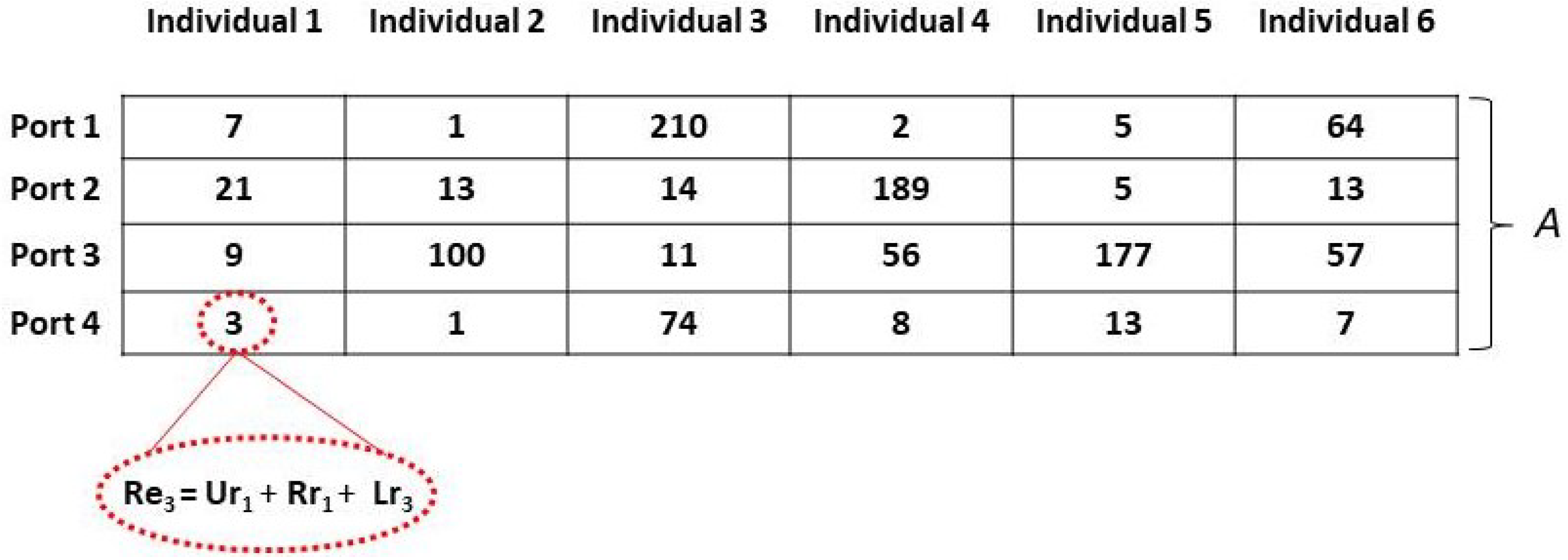
• $ExtractRules$: the function that defines the correspondence between the k rule, contained in $s\left(p\right)$ with the rules of unloading, loading, and retrieval to be stored in variables $U{r}_a$, $R{r}_e$, and $R{r}_e$, respectively;
• $nmov$: the total number of relocations performed.
• $Load$: the function that applies the ship’s loading operations through the concomitant execution of $R{r}_e$ and $R{r}_e$ rules. It returns the number of relocations made and the updated $Shp$ matrix.
• $Unload$: the function that defines the ship’s unloading operation through the execution of the $U{r}_a$ rule. It returns the number of relocations made and the updated $Shp$ matrix.

For each individual from the population, it was necessary to perform the simulation scheme described in Algorithm 1 to acquire its evaluation.

The second step of the evaluation method is to use the fitness measurement of each solution that was generated by the simulator and ensure that the best solutions were maintained in the population by the selection method.

This was accomplished by the following procedure. The best individual of all generations until the current one was kept for the next generations.

3.4.3. Selection

During the formation of the new population, some individuals from generation t were submitted to a transformation process by genetic operators to choose new rules. These transformations included unitary operators $m_i$ (mutation), which allowed the use of other rules by small changes in the individual attributes ($m_i:A_i\to A_i$), and superior order transformations $c_j$ (crossover), which produced new individuals by combining two individuals ($c_k:A_i\times A_j\to A_k$).

At the crossover, the single-point crossover method was applied. It consisted of randomly selecting a point in two parents’ chromosomes and swapping the two parent chromosomes to obtain new individuals.

At the mutation, every gene had a $m_i$ probability of being mutated. This was performed by randomly generating a value between 0 and 1. If it was lower than $m_i$, then a new value was generated for this gene within the set of permissible values, which in our case was any integer between 1 and 210.

This process was carried out until a previously specified maximum number of generations was reached [44,45]. It is important to remember that the notation proposed in this paper always generates feasible individuals, even after the selection operators are applied.

The next section describes the test instances used to validate the proposed method and the results obtained for these instances. Figure 10 illustrates how the described method works.

4. Results

Hereafter, we present the randomly generated test instances used to validate the method proposed and the results obtained with it.

As in [40], three types of instances were used, based on [24]: mixed-distance, short-distance, and long-distance instances. In the long-distance instances, all the containers traveled through many ports before being unloaded, staying onboard the ship for a relatively long period of time. In contrast, in the short-distance instances, the containers traveled through few ports before being unloaded and were, on average, onboard for a short period of time. In the mixed-distance instances, some containers traveled through several ports, and other containers traveled through few ports before being unloaded.

Another measure that could affect our problem was the occupancy rate ($OR$) of the yards. The more containers in the yard, the less space is available for performing relocation movements, which can make it more difficult to solve the problem.

Given this,

Table 1. Computational results for small- and medium-sized instances for a problem with five ports.

I	M	Yard			Ship			N	Results
		$\mathit{OR}$	H	W	R	C	B		$\mathit{OF}$	Time (s)
1	1	30%	4	5	2	3	3	24	1	0.38
2		60%			2	4	3	48	3	0.76
3		85%			3	5	3	68	12	1.40
4	2	30%	4	5	2	3	3	24	1	0.37
5		60%			2	4	3	48	5	0.83
6		85%			3	5	3	68	5	1.16
7	3	30%	4	5	2	4	3	24	3	0.59
8		60%			3	5	3	48	7	0.75
9		85%			3	6	3	68	8	1.56
10	1	30%	6	25	5	9	3	180	15	7.02
11		60%			6	12	3	360	47	22.05
12		85%			4	7	4	512	60	30.81
13	2	30%	6	25	4	7	3	180	14	4.44
14		60%			6	10	3	360	44	17.45
15		85%			6	12	3	512	82	22.28
16	3	30%	6	25	6	10	3	180	14	10.46
17		60%			6	11	4	360	39	15.86
18		85%			6	13	5	512	87	68.86

presents the computational results for the small- and medium-sized instances, and

Table 2. Computational results for large-sized instances for a problem with five ports.

I	M	Yard			Ship			N	Results
		$\mathit{OR}$	H	W	R	C	B		$\mathit{OF}$	Time (s)
19	1	30%	10	100	6	13	9	1200	137	123.93
20		60%			6	13	17	2400	374	436.46
21		85%			6	13	23	3400	701	804.09
22	2	30%	10	100	6	13	6	1200	124	89.57
23		60%			6	13	12	2400	350	300.79
24		85%			6	13	17	3400	687	662.38
25	3	30%	10	100	6	13	13	1200	126	108.24
26		60%			6	13	23	2400	364	474.69
27		85%			6	13	32	3400	680	668.10
28	1	30%	20	200	6	13	34	4800	734	2598.54
29		60%			6	13	66	9600	2183	3959.52
30		85%			6	13	95	13,600	4352	3649.01
31	2	30%	20	200	6	13	24	4800	726	1418.72
32		60%			6	13	47	9600	2202	3696.73
33		85%			6	13	67	13,600	4226	3969.72
34	3	30%	20	200	6	13	44	4800	730	2472.07
35		60%			6	13	87	9600	2296	3609.84
36		85%			6	13	124	13,600	4972	4022.46

presents the computational results for the large-sized instances. For both tables, column I indicates the instance number, and M indicates the instance type: 1 for mixed-distance, 2 for short-distance, and 3 for long-distance shipping. The $OR$ column gives the yard occupancy rate, and H and W indicate the number of rows and columns of the yard, respectively. Columns R, C, and B indicate the number of rows, columns, and bays of the ship, respectively. N shows the total number of containers which the ship dealt with throughout the entire problem. Finally, the objective function value ($OF$) is presented in terms of the number of relocations performed throughout the entire problem, and the $Time$ column provides the time in seconds that the proposed method took to solve the instance. In addition, the number of ports in the ship’s route was equal to five for all instances.

After many experiments, the chosen stopping criterion was the maximum number of 15 generations without any improvement to the objective function or when the maximum computational time of 1 h was reached. After these criteria, there was usually very little or no improvement in the objective function. Therefore, after reaching one of the conditions, the optimization problem was stopped, and the best solution obtained thus far was reported. Additionally, the population used had 10 individuals. The crossover operator was set to $c_j=0.8$ and the mutation operator to $m_i=0.3$. The implementation was performed in Python 3.8 and executed on a computer with an Intel Core™ i5-4210U (1.70 GHz) with 8 GB of RAM and using 4 threads.

From the results presented in Table 1 and Table 2, it can be seen that our solution was able to find good-quality feasible solutions for all instances within a reasonable computational time, especially when we consider the large number of rules that was evaluated by the method. From Table 1, one can see that all small- and medium-sized instances were solved in between a few seconds and six minutes. Meanwhile, most of the large-sized instances from Table 2 reached the maximum computational time of 1 h. It is worth remembering that instances of sizes of up to 500 containers are prohibitive for exact approaches since this generates an exorbitant number of variables, but they can be successfully solved by a personal computer when using the proposed approach.

In other approaches from the literature, such as [34,41], the biggest instances tested were of up to 10,000 containers and for a single CRP. In [10], the heuristic approach proposed was tested in instances of up to 700 containers, and the authors of [46] solved a single CRP with 45 containers.

Figure 11 and Figure 12 illustrate the evolution of the objective function of each instance (i.e., the total number of relocation movements of the best individual at each generation). Note that in a few instances, the GA could not improve the best solution of the first generation, but most instances had great improvements in the first generations. Nevertheless, the most important point is that good-quality solutions were obtained for the large-sized instances in low computational times, showing that the proposed approach can be applied in real case scenarios or even have commercial applications.

Note that in all instances, as the occupation of the yards increased, the computational time required to solve the problem also increased. When comparing the three types of transportation matrices, observe that the size required for the ship also depended on the type of matrix. When the containers stayed on the ship for more ports before being unloaded, more space was required to carry all the containers. When the containers stayed on the ship for only a few ports before being unloaded, less space was required. Due to these types of differences in the test instances, it is important to have a good variety of rules to be simulated, as we proposed.

Additionally, note that for the short-distance instances (type $M=2$), less time was required to finish the optimization, and fewer relocations were performed in most cases. Meanwhile, the long- and mixed-distance instances (types $M=3$ and $M=1$, respectively) took more computational time and relocations per instance.

These results show that the integration of the CRP with the ship MPSP must be considered to avoid a misleading analysis and unexpected extra relocation movements.

5. Conclusions and Future Works

This paper presented an extension of a methodology based on rules representation to solve the integration of the MPSP and the CRP at port yards.

As a contribution, the entire methodology was revised to provide a simpler representation of the problem. Some unpublished rules were presented, and a three-dimensional container ship was included. We were able to provide a faster evaluation of the possible actions via rules representation, whose associated binary model would not be feasible for a container yard with dimensions compatible with large ports.

As a result, good sequences of feasible movements were obtained within a short computational time. Moreover, we have demonstrated in detail that the container relocation problem should be considered when solving the multi-port stowage planning problem to ensure an efficient operation between the ship and port and prevent any loss of money.

For future works, we hope to extend the entire problem, including the scheduling of quay cranes, yard cranes, and vehicles, using a simulation and its respective rules. Another possible development is to couple the berth allocation problem and include the management of more than one ship in the simulation process. Finally, this simulation scheme also enables the consideration of uncertainty in processing times and the arrival of all equipment and structures related to the problem.

What-if scenarios varying the flow of containers at certain ports could be another interesting approach to effectively support the decision-making process.

Another objective function could also be considered, such as the distance traveled by the containers or total time to perform the operations. To solve a problem considering multiple objectives, multi-objective evolutionary algorithms such as NSGA or SPEA variants could also be implemented and have their results compared to the genetic algorithm proposed.

Finally, to improve performance, the problem could be employ a heuristic that considers groups of containers, and parallel processing could be implemented to provide faster evaluation of individuals through simulation. Furthermore, a comparison with other meta-heuristics in terms of computational performance could be carried out.

References

1. Ha, M.H.; Yang, Z.; Lam, J.S.L. Port performance in container transport logistics: A multi-stakeholder perspective. Transp. Policy 2019, 73, 25–40. [Google Scholar] [CrossRef]
2. Rahman, N.S.F.A.; Ismail, A.; Lun, V.Y. Preliminary study on new container stacking/storage system due to space limitations in container yard. Marit. Bus. Rev. 2016, 1, 21–39. [Google Scholar] [CrossRef]
3. Kang, J.G.; Kim, Y.D. Stowage planning in maritime container transportation. J. Oper. Res. Soc. 2002, 53, 415–426. [Google Scholar] [CrossRef]
4. Ambrosino, D.; Sciomachen, A.; Tanfani, E. A decomposition heuristics for the container ship stowage problem. J. Heuristics 2006, 12, 211–233. [Google Scholar] [CrossRef]
5. Parreño-Torres, C.; Alvarez-Valdes, R.; Parreño, F. Solution Strategies for a Multiport Container Ship Stowage Problem. Math. Probl. Eng. 2019, 2019, 9029267. [Google Scholar] [CrossRef]
6. Jin, B.; Zhu, W.; Lim, A. Solving the container relocation problem by an improved greedy look-ahead heuristic. Eur. J. Oper. Res. 2015, 240, 837–847. [Google Scholar] [CrossRef]
7. Chul-hwan, H. Assessing the impacts of port supply chain integration on port performance. Asian J. Shipp. Logist. 2018, 34, 129–135. [Google Scholar] [CrossRef]
8. Bierwirth, C.; Meisel, F. A follow-up survey of berth allocation and quay crane scheduling problems in container terminals. Eur. J. Oper. Res. 2015, 244, 675–689. [Google Scholar] [CrossRef]
9. Azevedo, A.T.; de Salles Neto, L.L.; Chaves, A.A.; Moretti, A.C. Solving the 3D stowage planning problem integrated with the quay crane scheduling problem by representation by rules and genetic algorithm. Appl. Soft Comput. 2018, 65, 495–516. [Google Scholar] [CrossRef]
10. Lee, Y.; Lee, Y.J. A heuristic for retrieving containers from a yard. Comput. Oper. Res. 2010, 37, 1139–1147. [Google Scholar] [CrossRef]
11. Boysen, N.; Briskorn, D.; Meisel, F. A generalized classification scheme for crane scheduling with interference. Eur. J. Oper. Res. 2016, 258, 343–357. [Google Scholar] [CrossRef]
12. Chang, D.; Fang, T.; Fan, Y. Dynamic rolling strategy for multi-vessel quay crane scheduling. Adv. Eng. Inform. 2017, 34, 60–69. [Google Scholar] [CrossRef]
13. Kizilay, D.; Eliiyi, D. A comprehensive review of quay crane scheduling, yard operations and integrations thereof in container terminals. Flex. Serv. Manuf. J. 2021, 33, 1–42. [Google Scholar] [CrossRef]
14. Yang, Y.; Zhong, M.; Dessouky, Y.; Postolache, O. An integrated scheduling method for AGV routing in automated container terminals. Comput. Ind. Eng. 2018, 126, 482–493. [Google Scholar] [CrossRef]
15. Niu, B.; Xie, T.; Tan, L.; Bi, Y.; Wang, Z. Swarm intelligence algorithms for Yard Truck Scheduling and Storage Allocation Problems. Neurocomputing 2016, 188, 284–293. [Google Scholar] [CrossRef]
16. Luo, J.; Wu, Y.; Mendes, A.B. Modelling of integrated vehicle scheduling and container storage problems in unloading process at an automated container terminal. Comput. Ind. Eng. 2016, 94, 32–44. [Google Scholar] [CrossRef]
17. Tan, C.; He, J.; Wang, Y. Storage yard management based on flexible yard template in container terminal. Adv. Eng. Inform. 2017, 34, 101–113. [Google Scholar] [CrossRef]
18. Kaysi, I.; Maddah, B.; Nehme, N.; Mneimneh, F. An integrated model for resource allocation and scheduling in a transshipment container terminal. Transp. Lett. 2012, 4, 143–152. [Google Scholar] [CrossRef]
19. Chen, L.; Langevin, A.; Lu, Z. Integrated scheduling of crane handling and truck transportation in a maritime container terminal. Eur. J. Oper. Res. 2013, 225, 142–152. [Google Scholar] [CrossRef]
20. Dotoli, M.; Epicoco, N.; Falagario, M.; Seatzu, C.; Turchiano, B. A Decision Support System for Optimizing Operations at Intermodal Railroad Terminals. IEEE Trans. Syst. Man Cybern. Syst. 2016, 47, 487–501. [Google Scholar] [CrossRef]
21. Cavone, G.; Dotoli, M.; Epicoco, N.; Seatzu, C. Intermodal terminal planning by Petri Nets and Data Envelopment Analysis. Control Eng. Pract. 2017, 69, 9–22. [Google Scholar] [CrossRef]
22. Iris, C.; Pacino, D. A Survey on the Ship Loading Problem. In Computational Logistics: 6th International Conference, ICCL 2015, Delft, The Netherlands, 23–25 September 2015, Proceedings; Corman, F., Voß, S., Negenborn, R.R., Eds.; Springer International Publishing: Cham, Switzerland, 2015; pp. 238–251. [Google Scholar] [CrossRef]
23. Zhao, N.; Mi, W.; Mi, C.; Chai, J. Study on Vessel Slot Planning Problem in Stowage Process of Outbound Containers. J. Appl. Sci. 2015, 13, 4278–4285. [Google Scholar] [CrossRef]
24. Avriel, M.; Penn, M.; Shpirer, N.; Witteboon, S. Stowage planning for container ships to reduce the number of shifts. Ann. Oper. Res. 1998, 76, 55–71. [Google Scholar] [CrossRef]
25. Ambrosino, D.; Paolucci, M.; Sciomachen, A. Computational evaluation of a MIP model for multi-port stowage planning problems. Soft Comput. 2017, 21, 1753–1763. [Google Scholar] [CrossRef]
26. Ding, D.; Chou, M.C. Stowage planning for container ships: A heuristic algorithm to reduce the number of shifts. Eur. J. Oper. Res. 2015, 246, 242–249. [Google Scholar] [CrossRef]
27. Dubrovsky, O.; Levitin, G.; Penn, M. A genetic algorithm with a compact solution encoding for the container ship stowage problem. J. Heuristics 2002, 8, 585–599. [Google Scholar] [CrossRef]
28. Gümüş, M.K.; Kaminsky, P.M.; Tiemroth, E.; Ayik, M. A Multi-stage Decomposition Heuristic for the Container Stowage Problem. In Proceedings of the 2008 MSOM Conference, College Park, MD, USA, 5–6 June 2008. [Google Scholar]
29. Pacino, D.; Delgado, A.; Jensen, R.M.; Bebbington, T. Fast Generation of Near-Optimal Plans for Eco-Efficient Stowage of Large Container Vessels. In Computational Logistics: Second International Conference, ICCL 2011, Hamburg, Germany, 19–22 September 2011, Proceedings; Böse, J.W., Hu, H., Jahn, C., Shi, X., Stahlbock, R., Voß, S., Eds.; Springer: Berlin/Heidelberg, Germany, 2011; pp. 286–301. [Google Scholar] [CrossRef]
30. Wilson, I.D.; Roach, P.A. Container Stowage Planning: A Methodology for Generating Computerized Solutions. J. Oper. Res. Soc. 2000, 51, 1248–1255. [Google Scholar] [CrossRef]
31. Monaco, M.F.; Sammarra, M.; Sorrentino, G. The terminal-oriented ship stowage planning problem. Eur. J. Oper. Res. 2014, 239, 256–265. [Google Scholar] [CrossRef]
32. Çaǧatay, I.; Christensen, J.; Pacino, D.; Ropke, S. Flexible ship loading problem with transfer vehicle assignment and scheduling. Transp. Res. Part B Methodol. 2018, 111, 113–134. [Google Scholar] [CrossRef]
33. Ji, M.; Guo, W.; Zhu, H.; Yang, Y. Optimization of loading sequence and rehandling strategy for multi-quay crane operations in container terminals. Transp. Res. Part E 2015, 80, 1–19. [Google Scholar] [CrossRef]
34. Caserta, M.; Schwarze, S.; VoSS, S. A mathematical formulation and complexity considerations for the blocks relocation problem. Eur. J. Oper. Res. 2012, 219, 96–104. [Google Scholar] [CrossRef]
35. Junqueira, C.; Quiñones, M.P.; de Azevedo, A.T.; Rocco, C.D.; Ohishi, T. An Integrated Optimization Model for the Multi-Port Stowage Planning and the Container Relocation Problems. arXiv 2020, arXiv:2006.06795. [Google Scholar]
36. Azevedo, A.T.D.; Ribeiro, C.M.; Sena, G.J.D.; Chaves, A.A.; Neto, L.L.S.; Moretti, A.C. Solving the 3D Container Ship Loading Planning Problem by Representation by Rules and Meta-heuristics. Int. J. Data Anal. Tech. Strateg. 2014, 6, 228–260. [Google Scholar] [CrossRef]
37. Burke, E.K.; Gendreau, M.; Hyde, M.; Kendall, G.; Ochoa, G.; Özcan, E.; Qu, R. Hyper-heuristics: A survey of the state of the art. J. Oper. Res. Soc. 2013, 64, 1695–1724. [Google Scholar] [CrossRef]
38. Drake, J.H.; Kheiri, A.; Özcan, E.; Burke, E.K. Recent advances in selection hyper-heuristics. Eur. J. Oper. Res. 2020, 285, 405–428. [Google Scholar] [CrossRef]
39. Azevedo, A.; Arruda, E.; Leduino, L.; Neto, S.; Chaves, A.; Moretti, A. Application of the Participatory Learning System to Solve the Problem of Loading and Unloading 3D Containers at Port Terminals for Multiple Scenarios. Pesqui. Nav. 2016, 27, 57–68. [Google Scholar]
40. Junqueira, C.; Azevedo, A.T.; Ohishi, T. Stowage Planning and Storage Space Assignment of Containers in Port Yards. IX COPEDEC 2016, 9, 1248–1255. [Google Scholar]
41. Petering, M.E.H.; Hussein, M.I. A new mixed integer program and extended look-ahead heuristic algorithm for the block relocation problem. Eur. J. Oper. Res. 2013, 231, 120–130. [Google Scholar] [CrossRef]
42. Araujo, E.J.; Chaves, A.A.; de Salles Neto, L.L.; de Azevedo, A.T. Pareto clustering search applied for 3D container ship loading plan problem. Expert Syst. Appl. 2016, 44, 50–57. [Google Scholar] [CrossRef]
43. Meisel, F.; Wichmann, M. Container sequencing for quay cranes with internal reshuffles. OR Spectr. 2010, 32, 569–591. [Google Scholar] [CrossRef]
44. Holland, J.H. Adaptation in Natural and Artificial Systems; The University of Michigan Press: Ann Arbor, MI, USA, 1975. [Google Scholar]
45. Michalewicz, Z. Genetic Algorithms + Data Structures = Evolution Programs, 3rd ed.; Springer: Berlin/Heidelberg, Germany, 1996. [Google Scholar] [CrossRef]
46. Lee, Y.; Hsu, N.Y. An optimization model for the container pre-marshalling problem. Comput. Oper. Res. 2007, 34, 3295–3313. [Google Scholar] [CrossRef]
Figure 1. Loading flow at port 1.
Applsci 12 08191 g001
Figure 2. Unloading flow at port 2.
Applsci 12 08191 g002
Figure 3. Loading flow at port 2.
Applsci 12 08191 g003
Figure 4. Yard relocation rules’ searching flows. (a) Rule R r 1 . (b) Rule R r 2 . (c) Rule R r 3 . (d) Rule R r 4 . (e) Rule R r 5 . (f) Rule R r 6 .
Applsci 12 08191 g004
Figure 5. Representation of the use of rule R r 8 .
Applsci 12 08191 g005
Figure 6. Ship loading rules’ searching flows. (a) Rule L r 1 . (b) Rule L r 2 . (c) Rule L r 3 . (d) Rule L r 4 .
Applsci 12 08191 g006
Figure 7. Ship loading rules’ searching flows. (a) Rule L r 5 . (b) Rule L r 6 . (c) Rule L r 7 . (d) Rule L r 8 .
Applsci 12 08191 g007
Figure 8. Rules produced by combining retrieval, loading, and unloading rules.
Applsci 12 08191 g008
Figure 9. Representation of the b best solutions in a population of six individuals within a matrix.
Applsci 12 08191 g009
Figure 10. Representation of the proposed method.
Applsci 12 08191 g010
Figure 11. Evolution of the objective function of small- and medium-sized instances.
Applsci 12 08191 g011
Figure 12. Evolution of the objective function of large-sized instances.
Applsci 12 08191 g012