Fitmix: An R Package for Mixture Modeling of the Budding Yeast S. cerevisiae Replicative Lifespan (RLS) Distributions

Abstract

Replicative lifespan (RLS) of the budding yeast is the number of mother cell divisions until senescence and is instrumental to understanding mechanisms of cellular aging. Recent research has shown that replicative aging is heterogeneous, which argues for mixture modeling. The mixture model is a statistical method to infer subpopulations of the heterogeneous population. Mixture modeling is a relatively underdeveloped area in the study of cellular aging. There is no open access software currently available that assists extensive comparison among mixture modeling methods. To address these needs, we developed an R package called fitmix that facilitates the computation of well-known distributions utilized for RLS data and other lifetime datasets. This package can generate a group of functions for the estimation of probability distributions and simulation of random observations from well-known finite mixture models including Gompertz, Log-logistic, Log-normal, and Weibull models. To estimate and compute the maximum likelihood estimates of the model parameters, the Expectation–Maximization (EM) algorithm is employed.

1. Introduction

An increase in mortality rate is typically interpreted as aging. In cellular aging, the budding yeast S. cerevisiae has revealed many significant properties in the mechanism of eukaryotic lifespan regulation [1,2,3]. Studies of yeast aging have led to many conserved components that affect lifespan [2,4,5]. Yeast lifespan is typically measured by two different approaches. The first is chronological lifespan (CLS), defined as the duration of time that a mother cell remains alive without division. The second is the replicative lifespan (RLS) of a mother cell, calculated as the number of mother cell divisions until senescence [6]. Historically, analysis of the RLS data has been conducted with nonparametric methods or using typical parametric survival models [7]. Survival analysis of the lifespan datasets has been generally delineated with the standard lifespan statistical distributions such as Gompertz, Weibull, Logistic, and Log-logistic [8]. In addition to these conventional statistical distribution models, several models for RLS data of budding yeast have been recently published [9].

Recent studies show that yeast replicative aging is heterogeneous and contains at least two subpopulations [10,11], which argues for mixture models. Finite mixtures are studied and applied to several applications, especially in biological (failure data) and medical (disease distributions) areas since the end of the 19th century. Both grouped and ungrouped datasets are aimed at the calculation of the parameters of finite mixtures [12].

Heterogeneous distributions of mixture population models such as the budding yeast S. cerevisiae can be utilized to model a population with subpopulations. Insights might be gained by comparing the mixture models of the wildtypes, mutants, and various treatments such as calorie restriction. The mixture survival analysis of the RLS of a cell is a compilation of statistical approaches for lifespan data analysis of mixture models expressing heterogeneous states of yeast cell populations with diverse genotypes. In a complete population, mixture components are the densities (probabilities) of the subpopulations, and weights are represented by the fraction of each subpopulation in the complete population.

Frequency distribution is useful in the instance of single-mode survival lifespan data with the conventional probability distribution model [9,13,14]. The mixture of probability density functions is even more advantageous since it is used to portray a heterogeneous lifetime dataset when there is an indication of simple bimodality or multimodality [15,16].

The RLSs of the budding yeast distributions are not sufficiently portrayed by a single probability distribution since mother cell decrease is related to asymmetric phenotypes such as dysregulation of vacuole acidity, genomic instability, and partial reservation of protein aggregates [3,6,17]. In such settings, often finite mixture distributions are used to describe complex and multi-modal asymmetric division distributions.

Marin et al. (2005) propose a mixture of Weibull models utilizing Bayesian analysis to model the heterogeneous lifespans [18], generalizing an earlier finding that Tsionas (2002) studied Weibull distributions of a finite mixture with a fixed number of components [19]. In Al-Hussaini et al. (1999), a finite mixture model of a Gompertz component and a surviving portion in the framework of Types I and II censored samples from heterogeneous population is considered [20].

The basic goal of the functions of fitmix, which is an open-source R package, is to offer a confined set of models to fit a diverse lifespan, even with large datasets, specifically the replicative lifespan of budding yeast or other biological units. It is a publicly accessible software published on 2021-04-19 and obtainable at https://cran.r-project.org/web/packages/fitmix/index.html (accessed on 18 March 2021) on the Comprehensive R Archive Network (CRAN) protected with a GPL3 license. Specifically, functions are intended to facilitate comparison between parameter estimation techniques and models, utilizing a set of models of mixture fit standards, without requiring an in-depth understanding of the statistical computations and coding skills performed in the estimation procedure.

The fitmix package would have prompt use in biostatistics and bioinformatics, in addition to other biological and medical areas in which mixture modeling lifespan, survival, and lifetime distributions are a significant task (e.g., cancer survival data, disease datasets, and lifespan datasets of single units). This study aims to characterize the practicality of the fitmix package and demonstrate its traits using the analysis of yeast replicative lifespan data [9,14,21].

2. Materials and Methods

2.1. Survival Time Functions

Let T $\ge 0$ be a continuous random variable, i.e., the survival time, and let F(t) be a cumulative distribution function on the $\left[0, \infty \right)$ interval. The continuous variable T distribution can be defined by three functions. First is $\mathrm{F}\left(\mathrm{t}\right)$, which is a cumulative of $\mathrm{T}$,

$$\mathrm{F}\left(\mathrm{t}\right)=\mathrm{P}\left(\mathrm{T}\le \mathrm{t}\right)$$

(1)

where t is $0\le$ $\mathrm{t}<\infty$. P is called the probability that the random variable $\mathrm{T}\le \mathrm{t}.$ F(t) represents the definition of the cumulative distribution function that an individual fails before t.

The other function is S(t), which is the survival (reliability) function and can be described as the probability that a biological trait endures longer than t:

$$\mathrm{S}\left(\mathrm{t}\right)=\mathrm{P}\left(\left\{\mathrm{T}>\mathrm{t}\right\}\right)={\int }_1^{\infty }\mathrm{f}\left(\mathrm{x}\right)\mathrm{dx}=1-\mathrm{F}\left(\mathrm{t}\right),$$

(2)

where S(t) is a non-increasing function of time t used to describe and demonstrate the survival data (RLS).

The h(t) function is called the hazard function and expresses the death rate for an item of a survival time t. The h(t) function analyzes the probability of survival at a given point in time, based on whether an item survives to an earlier time t. In other words, it is the probability that if something survives one moment, it will also survive the next. This turns into an instantaneous hazard rate as $\mathsf{\Delta }\mathrm{t}$ leads to zero:

$$\mathrm{h}\left(\mathrm{t}\right)=\underset{\mathsf{\Delta }\mathrm{t}\to 0}{\lim }\frac{\mathrm{S}\left(\mathrm{t}\right)-\mathrm{S}\left(\mathrm{t}+\mathsf{\Delta }\mathrm{t}\right)}{\mathsf{\Delta }\mathrm{t}. \mathrm{S}\left(\mathrm{t}\right)}=\frac{\mathrm{f}\left(\mathrm{t}\right)}{\mathrm{S}\left(\mathrm{t}\right)}$$

(3)

The cumulative hazard function $\mathrm{H}\left(\mathrm{t}\right)$, on the other hand, is defined as

$$\mathrm{H}\left(\mathrm{t}\right)=-\log \left(\mathrm{S}\left(\mathrm{t}\right)\right)={\int }_0^{\mathrm{t}}\mathrm{h}\left(\mathrm{x}\right)\mathrm{dx}.$$

(4)

The CDF $\mathrm{F}\left(\mathrm{t}\right)$ can be used to calculate the probability of failure, which is simply a continuous failure depending on a failure distribution

$$\mathrm{P}\left(\mathrm{T}\le \mathrm{t}\right)=\mathrm{F}\left(\mathrm{t}\right)=1-\mathrm{S}\left(\mathrm{t}\right).$$

(5)

2.1.1. Gompertz Distribution

Failure (mortality) rate in biological aging usually follows the Gompertz distribution, i.e., an exponential law. The Gompertz distribution with a provided PDF and CDF is determined as

$${ \mathrm{f}}_{\mathrm{R},\mathrm{G}}\left(\mathrm{t}\right)={\mathrm{Re}}^{\mathrm{Gt}}\exp \left[\frac{\mathrm{R}}{\mathrm{G}} \left(1-{\mathrm{e}}^{\mathrm{Gt}}\right)\right] \mathrm{and} { \mathrm{F}}_{\mathrm{R},\mathrm{G}}\left(\mathrm{t}\right)=1- \exp \left[\frac{\mathrm{R}}{\mathrm{G}} \left(1-{\mathrm{e}}^{\mathrm{Gt}}\right)\right]$$

where R and G are the rate and shape parameters, respectively.

Further, the survival (viability) and hazard functions of the Gompertz distribution are given by

$$\mathrm{S}\left(\mathrm{t}\right)=\exp \left(-\frac{\mathrm{R}}{\mathrm{G}}\left({\mathrm{e}}^{\mathrm{Gt}}-1\right)\right) \mathrm{and} \mathrm{H}\left(\mathrm{t}\right)=\mathrm{R} \exp \left(\mathrm{Gt}\right), \mathrm{respectively}.$$

2.1.2. Log-Logistic Distribution

The Log-logistic distribution is also a power law. It can be utilized to fit the lifetime of an object, a service, or an organism. The Log-logistic model with a provided PDF and CDF is determined as

$${ \mathrm{f}}_{\mathsf{\lambda },\mathsf{\kappa }}\left(\mathrm{t}\right)=\frac{\mathsf{\lambda }\mathsf{\kappa }{\left(\mathsf{\lambda }\mathrm{t}\right)}^{\mathsf{\kappa }-1}}{{(1+{\left(\mathsf{\lambda }\mathrm{t}\right)}^{\mathsf{\kappa }})}^2} \mathrm{and} { \mathrm{F}}_{\mathsf{\lambda },\mathsf{\kappa }}\left(\mathrm{t}\right)={\left(1+{\left(\frac{\mathsf{\lambda }}{\mathrm{t}}\right)}^{\mathsf{\kappa }}\right)}^{-1}$$

respectively, where λ and κ > 0 are the scale and shape parameters of each. Further, the survival (viability) and hazard functions of Log-logistic distribution are provided by

$$\mathrm{S}\left(\mathrm{t}\right)=\frac{1}{1+{\mathsf{\lambda }\mathrm{t}}^{\mathsf{\kappa }}} \mathrm{and} \mathrm{H}\left(\mathrm{t}\right)=\frac{{\mathsf{\lambda }\mathsf{\kappa }\mathrm{t}}^{\mathsf{\kappa }-1}}{1+{\mathsf{\lambda }\mathrm{t}}^{\mathsf{\kappa }}}, \mathrm{respectively}$$

2.1.3. Log-Normal Distribution

In a Log-normal distribution case, the natural logarithm ($\ln \left(\mathrm{t}\right)$) of the lifespan t is supposed to be normally distributed. The Log-normal model with a given PDF defined as

$${ \mathrm{f}}_{\mathsf{\mu },\mathsf{\sigma }}\left(\mathrm{t}\right)=\frac{1}{\sqrt{2}\mathsf{\pi } \mathsf{\sigma }\mathrm{t}}\frac{\exp {\left(-(\ln \left(\mathrm{t}\right)-\mathsf{\mu }\right)}^2}{2{\mathsf{\sigma }}^2}$$

(6)

where mean is $\mathrm{Et}={\mathrm{e}}^{\mathsf{\mu }}+\frac{{\mathsf{\sigma }}^2}{2}$ and variance is $\mathrm{V}\left(\mathrm{t}\right)={\mathrm{e}}^{2\mathsf{\mu }+{\mathsf{\sigma }}^2}\left({\mathrm{e}}^{{\mathsf{\sigma }}^2}-1\right)$.

The Log-normal distribution generally is used with non-censored data. However, as this distribution is employed for censored data, calculations may become difficult provided that the hazard function

$$\mathrm{H}\left(\mathrm{t},\mathsf{\sigma }\right)=\frac{ \frac{1}{\sqrt{2\mathsf{\pi }} \mathsf{\sigma }\mathrm{t}}{\mathrm{e}}^{-1/2{\left(\frac{\ln \mathrm{t}-\mathsf{\mu }}{\mathsf{\sigma }}\right)}^2} }{1-\mathsf{\phi }\left[\frac{\ln \mathrm{t}-\mathsf{\mu }}{\mathsf{\sigma }}\right]},$$

(7)

gives zero at $\mathrm{t} =0$, increases to a maximum, and then decreases, getting close to zero as t leads to infinity.

2.1.4. Weibull Distribution

Mortality (failure) rate in machinery senescence usually follows the Weibull (a power law) model of aging. The Weibull model with a provided PDF and CDF can be explained as

$${ \mathrm{f}}_{\mathsf{\theta },\mathsf{\gamma }}\left(\mathrm{t}\right)={\mathsf{\gamma }\mathsf{\theta }}^{\mathsf{\gamma }}{ \mathrm{t}}^{\mathsf{\gamma }-1 }\exp {\left(-\mathsf{\theta }\mathrm{t}\right)}^{\mathsf{\gamma }}, \mathrm{and} { \mathrm{F}}_{\mathsf{\theta },\mathsf{\gamma }}\left(\mathrm{t}\right)=1-{\mathrm{e}}^{-{\left(\mathsf{\theta }\mathrm{t}\right)}^{\mathsf{\gamma }}}$$

respectively, where t > 0, and θ and γ are the scale and shape parameters, respectively. Moreover, the survival and hazard functions are given by

$$\mathrm{s}\left(\mathrm{t}\right)=\exp {\left(-\mathsf{\theta }\mathrm{t}\right)}^{\mathsf{\gamma }} \mathrm{and} \mathrm{H}\left(\mathrm{t}\right)={\mathsf{\theta } \mathsf{\gamma } \mathrm{t}}^{\mathsf{\gamma }-1}, \mathrm{respectively}.$$

2.2. General Case for the Mixture Model

The CDF, PDF, and HF of a typical $\mathsf{\kappa }$-parameter mixture model consisting of $\mathsf{\kappa }$ subpopulations (subgroups or subclasses) have been presented by Blischke et al. (2011) [22]. A $\mathsf{\kappa }$-parameter finite mixture model of the CDF can be characterized as

$$\mathrm{G}\left(\mathrm{t}\right)={\displaystyle \sum }_{\mathrm{j}=1}^{\mathrm{K}}{\mathrm{p}}_{\mathrm{j}}{ \mathrm{F}}_{\mathrm{j}}\left(\mathrm{t}\right)$$

(8)

where F_j(t) is the CDF and p_j is the probability of the mixture of jth subpopulation, where p_j > 0 and ${\displaystyle \sum }_{\mathrm{j}=1}^{\mathrm{K}}{\mathrm{p}}_{\mathrm{j}}=1$. The PDF is given by

$$\mathrm{g}\left(\mathrm{t}\right)=\sum _{\mathrm{j}=1}^{\mathrm{K}}{\mathrm{p}}_{\mathrm{j}} \mathrm{f}\left(\mathrm{t}\right)$$

(9)

where f_j(t) is the probability density function related to F_j(t). The HF is

$$\mathrm{H}\left(\mathrm{t}\right)=\sum _{\mathrm{j}=1}^{\mathrm{K}}{\mathrm{w}}_{\mathrm{j}}\left(\mathrm{t}\right){\mathrm{h}}_{\mathrm{j}}\left(\mathrm{t}\right)$$

(10)

where h_j(t) represents subpopulation j, and

$${\mathrm{w}}_{\mathrm{j}}\left(\mathrm{t}\right)=\frac{{\mathrm{p}}_{\mathrm{j}}{\mathrm{R}}_{\mathrm{j}}\left(\mathrm{t}\right)}{{\sum }_{\mathrm{j}=1}^{\mathrm{K}}{\mathrm{p}}_{\mathrm{j}}{\mathrm{R}}_{\mathrm{j}}\left(\mathrm{t}\right)}, \mathrm{j}=1, 2,\dots , \mathrm{K}$$

(11)

where $\sum _{\mathrm{j}=1}^{\mathrm{K}}{\mathrm{w}}_{\mathrm{j}}\left(\mathrm{t}\right)=1$ with

$${ \mathrm{R}}_{\mathrm{j}}\left(\mathrm{t}\right)=1-{\mathrm{F}}_{\mathrm{j}}\left(\mathrm{t}\right), \mathrm{j}=1, 2,\dots , \mathrm{K}$$

(12)

For the subpopulations with the weights, it can be followed from Equation (3) that the failure rate for the given distribution is a weighted mean of the failure rate varying with $\mathrm{t}, \mathrm{t}\ge 0$.

2.3. An Example: Deriving Gompertz Mixture Model

The CDF of the two-parameter mixture model for K = 2 in Equation (1) for the random variable is given by

G(t) = pF1(t) + (1 − p)F2(t),  t ≥ 0

(13)

If F₁(t) follows Gompertz $\left({\mathrm{R}}_1,{\mathrm{G}}_1\right)$ and F₂(t) follows Gompertz $\left({\mathrm{R}}_2,{\mathrm{G}}_2\right)$ distributions, the CDF for the two-parameter Gompertz mixture model from Equation (8) becomes

$$\begin{array}{cc}\mathrm{G}\left(\mathrm{t}\right)=\hfill & \left[1-\exp \left(-\frac{{\mathrm{R}}_2}{{\mathrm{G}}_2}\left({\mathrm{e}}^{{\mathrm{G}}_2\mathrm{t}}-1\right)\right)\right]\hfill \\ & +\mathrm{p}\left[\exp \left(-\frac{{\mathrm{R}}_2}{{\mathrm{G}}_2}\left({\mathrm{e}}^{{\mathrm{G}}_2\mathrm{t}}-1\right)\right)-\exp \left(-\frac{{\mathrm{R}}_1}{{\mathrm{G}}_1}\left({\mathrm{e}}^{{\mathrm{G}}_1\mathrm{t}}-1\right)\right)\right],\hfill \\ & \left\{{\mathrm{R}}_1,{ \mathrm{G}}_1,{\mathrm{R}}_2,{\mathrm{G}}_2\right\}>0,\mathrm{t}\ge 0\end{array}$$

(14)

$$\begin{gathered} \mathrm{g}\left(\mathrm{t}\right)={\mathrm{R}}_2{\mathrm{e}}^{{\mathrm{G}}_2\mathrm{t}}\exp \left( \frac{{\mathrm{R}}_2}{{\mathrm{G}}_2} \left(1-{\mathrm{e}}^{{\mathrm{G}}_2\mathrm{t}}\right)\right) \\ +\mathrm{p}\left[{\mathrm{R}}_1{\mathrm{e}}^{{\mathrm{G}}_1\mathrm{t}} \exp \left(\frac{{\mathrm{R}}_1}{{\mathrm{G}}_1} \left(1-{\mathrm{e}}^{{\mathrm{G}}_1\mathrm{t}}\right)\right)-{\mathrm{R}}_2{\mathrm{e}}^{{\mathrm{G}}_2\mathrm{t}}\exp \left(\frac{{\mathrm{R}}_2}{{\mathrm{G}}_2} \left(1-{\mathrm{e}}^{{\mathrm{G}}_2\mathrm{t}}\right)\right)\right], \mathrm{t}\ge 0 \end{gathered}$$

(15)

The hazard function is

$$\mathrm{h}\left(\mathrm{t}\right)=\frac{{\mathrm{pf}}_1\left(\mathrm{t}\right)+\left(1-\mathrm{p}\right){ \mathrm{f}}_2\left(\mathrm{t}\right)}{\mathrm{p} \exp \left(\frac{{\mathrm{R}}_1}{{\mathrm{G}}_1} \left(1-{\mathrm{e}}^{{\mathrm{G}}_1\mathrm{t}}\right)\right)+\left(1-\mathrm{p}\right) \exp \left(\frac{{\mathrm{R}}_2}{{\mathrm{G}}_2} \left(1-{\mathrm{e}}^{{\mathrm{G}}_2\mathrm{t}}\right)\right)}, \mathrm{t}\ge 0$$

(16)

Analogously, by utilizing different CDFs from different time distributions, other $\mathsf{\kappa }$-component mixture models can be derived.

2.4. Maximum Likelihood Estimations of the Parameters with EM Algorithm in Mixture of Distributions

The EM algorithm has been applied as an approach to estimate and compute the parameters by the method of maximum likelihood in the finite mixture models [23]. In the EM framework, the realizations ${\mathrm{t}}_1,\dots {\mathrm{t}}_{\mathrm{n}}$ are considered as partial data and implicit class variables ${\mathrm{z}}_1,\cdots {\mathrm{z}}_{\mathrm{g}}$ to be non-present where ${\mathrm{z}}_{\mathrm{ki}}={ \mathrm{z}}_{\mathrm{k}}\left({\mathrm{t}}_{\mathrm{i}}\right)=1$ if observation ${\mathrm{t}}_{\mathrm{i}}$ is included at the $\mathrm{kth}$ class, and $0$ otherwise for $\mathrm{k}=1,\cdots ,\mathrm{g}$ and $\mathrm{i}=1,\cdots , \mathrm{n}$.

The EM algorithm is used in the mixture distributions by processing z as non-present data.

2.5. Estimating the Parameters of Replicative Lifespan Datasets Fitted by Mixture Models

In addition to modeling lifespan distributions, describing the link between replicative lifespan of genetic backgrounds is a significant mission for acquiring precise lifespan extension and failure measurements. For instance, the Weibull model is useful to infer the emergence characteristics of aging during the initial life stage. Most of the survival functions, such as the logistic function, are studied in late life during aging [24].

Whereas, the Log-normal model behaves differently since the model is not suitable for lifetime modeling where hazards increase with old age. Regardless of its revolting features, the Log-normal distribution has been broadly employed as a failure distribution in several cases, such as the analysis of electrical isolation or time to develop lung cancer among smokers. Moreover, the Log-normal distribution has often been used as a mixture model [25].

2.6. Goodness-of-Fit Measurement of Mixture Modeling

Deciding on the number of components is one of the most significant issues in fitting heterogeneous distributions with mixture models [25]. In mixture models, the number of components can be defined with a variety of criteria. The fitmix package utilizes four approaches to assess the performance of fitted models. Given a collection of mixture models for the RLS (lifetime or survival data), the measurements of four goodness-of-fits can be listed as Akaike Information Criterion (AIC), Bayesian Information Criterion (BIC), Kolmogorov–Smirnov (KS), and log-likelihood (log.likelihood) statistics.

2.6.1. Akaike Information Criterion (AIC)

AIC is commonly used to assess the performance of distinct mixture models. Therefore, AIC yields a mean for a (mixture) model selection. The user can implement AIC for defining the number of components.

The AIC measure is defined by the maximum likelihood estimation of the model as a measure of fit,

$$\mathrm{AIC}=-2 \ln \left(\mathrm{L}\right)+2\mathrm{k}$$

(17)

where L is the maximized value of likelihood function and k is the number of parameters of finite mixture model [16,26].

2.6.2. Bayesian Information Criterion (BIC)

Bayesian information criterion (BIC) is one of the goodness-of-fit measurements for the selection of a (mixture) model among finite (mixture) models. It is based on the maximum likelihood estimation procedure and closely related to AIC. It is likely to increase the value of likelihood by including more parameters, which might result in overfitting. The BIC settles the overfitting issue by inserting a penalty term for the number of parameters in the chosen model. The value of the penalty term is smaller in AIC than in BIC.

$$\mathrm{BIC}=\mathrm{k} \ln \left(\mathrm{n}\right)-2 \ln \left(\mathrm{L}\right)$$

(18)

where k is the number of parameters, n is the number of data points in RLS (lifetime or survival time), and L is a value which is the maximum value of likelihood function in the finite mixture model [27].

2.6.3. Kolmogorov–Smirnov (KS)

As in the other goodness-of-fit measurements, the Kolmogorov–Smirnov measurement allows for comparison between different models and is used to determine if RLS data (lifetime or survival data) arises from a population with a specific distribution [28]. Although KS is non-parametric, it can be utilized to check the analysis of variance under the assumption of normality.

When the size of lifetime data is small enough, KS can be used to compare a variable of the cumulative distribution function with a particular distribution. The value of test statistic D is calculated with the assumption of the null hypothesis of no difference between the theoretical distribution and empirical data as

$$\mathrm{D}=\max \left|{\mathrm{F}}_{\mathrm{o}}\left(\mathrm{t}\right)-{\mathrm{F}}_{\mathrm{r}}\left(\mathrm{t}\right)\right|$$

(19)

where ${\mathrm{F}}_{\mathrm{o}}\left(\mathrm{t}\right)=\frac{\mathrm{k}}{\mathrm{n}}$ is the empirical distribution function (eCDF) of n, n is the total number of realizations in which $\mathrm{k}$ is the number of realizations, with $\mathrm{k}\le \mathrm{T}$, and ${\mathrm{F}}_{\mathrm{r}}\left(\mathrm{t}\right)$ is the cumulative distribution function (CDF). The D value is subject to the KS test table.

2.6.4. The Log-Likelihood Test

The log-likelihood function is a natural logarithmic transformation of the likelihood function, which is the method of obtaining the unknown parameters of a (mixture) model via the maximum of likelihood function. It is one of the measures of goodness-of-fit of a theoretical distribution to lifetime data points for unknown parameters [29]. In the lifetime or survival time case, generally, the likelihood function is defined as discrete distributions.

Given a model of probability density functions $\mathrm{t}\mapsto \mathrm{f}\left(\mathrm{t}\mathsf{\alpha },\mathsf{\beta }\right)$ where $\mathsf{\alpha },\mathsf{\beta }$ are the parameters, the likelihood function is $\mathsf{\alpha },\mathsf{\beta }\mapsto \mathrm{f}\left(\mathrm{t}\mid \mathsf{\alpha },\mathsf{\beta }\right)$ and can be written as

$$ℒ\left(\mathsf{\alpha },\mathsf{\beta }|\mathrm{t}\right)=\mathrm{f}(\mathrm{t}|\mathsf{\alpha },\mathsf{\beta }),$$

(20)

where $\mathrm{t}>0$ are the discrete data points of the lifetime.

The log-likelihood function of the chosen model for the given PDF is as follows:

$$\log \left(\mathrm{L}\left(\mathsf{\alpha },{\mathsf{\beta }|\mathrm{t}}_{\mathrm{i}}\right)\right)= \mathrm{LL}\left(\mathsf{\alpha },{\mathsf{\beta }|\mathrm{t}}_{\mathrm{i}}\right)={{\displaystyle \sum }}_{\mathrm{i}=1}^{\mathrm{N}}\log \left[{\mathrm{f}}_{\mathsf{\alpha },\mathsf{\beta }}\left({\mathrm{t}}_{\mathrm{i}}\right)\right]$$

(21)

$$\mathrm{LL}\left(\mathsf{\alpha },\mathsf{\beta }|{\mathrm{t}}_{\mathrm{i}}\right)=\mathrm{LL}\left({\mathrm{f}}_{\mathsf{\alpha },\mathsf{\beta }}\left({\mathrm{t}}_{\mathrm{i}}\right)\right)$$

(22)

3. Results

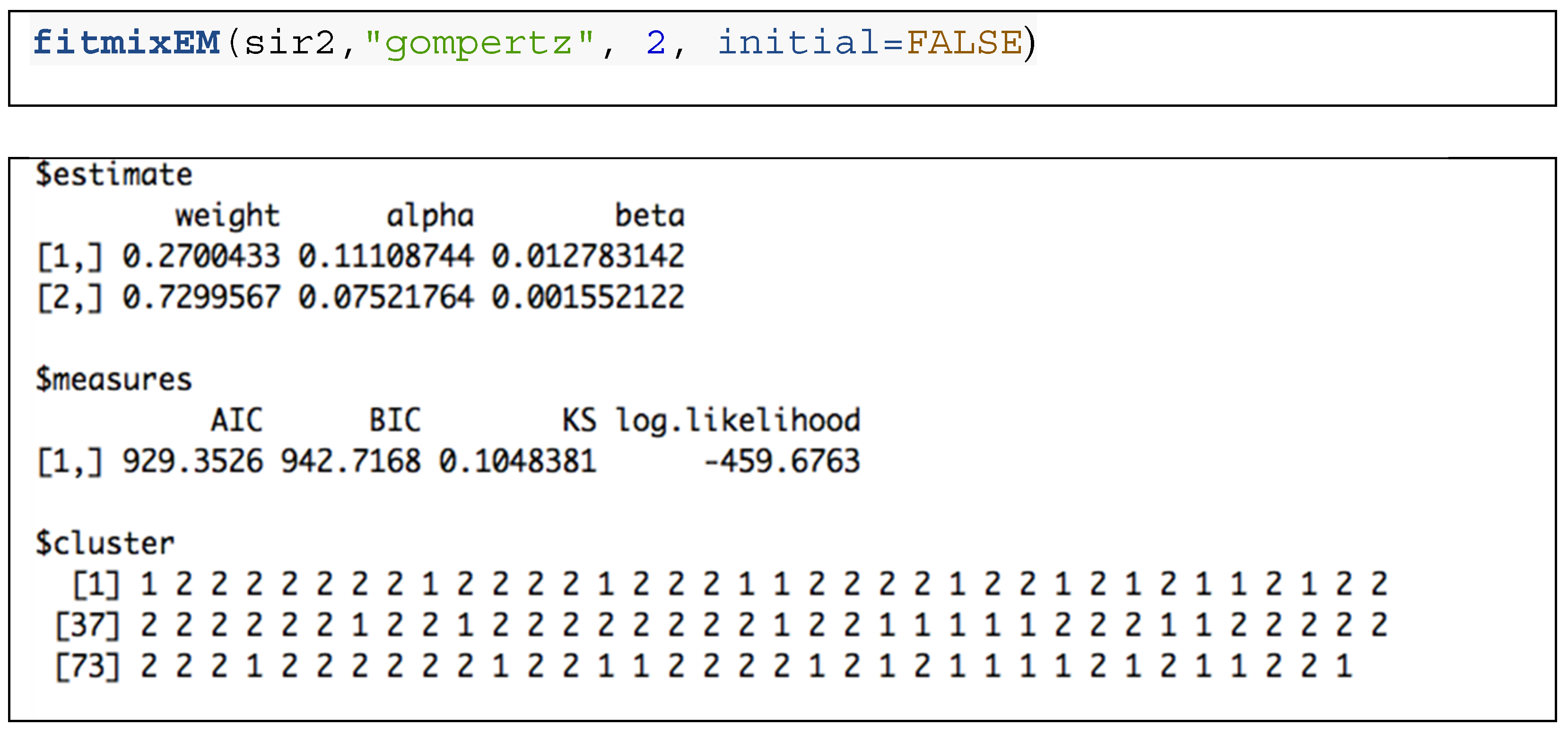
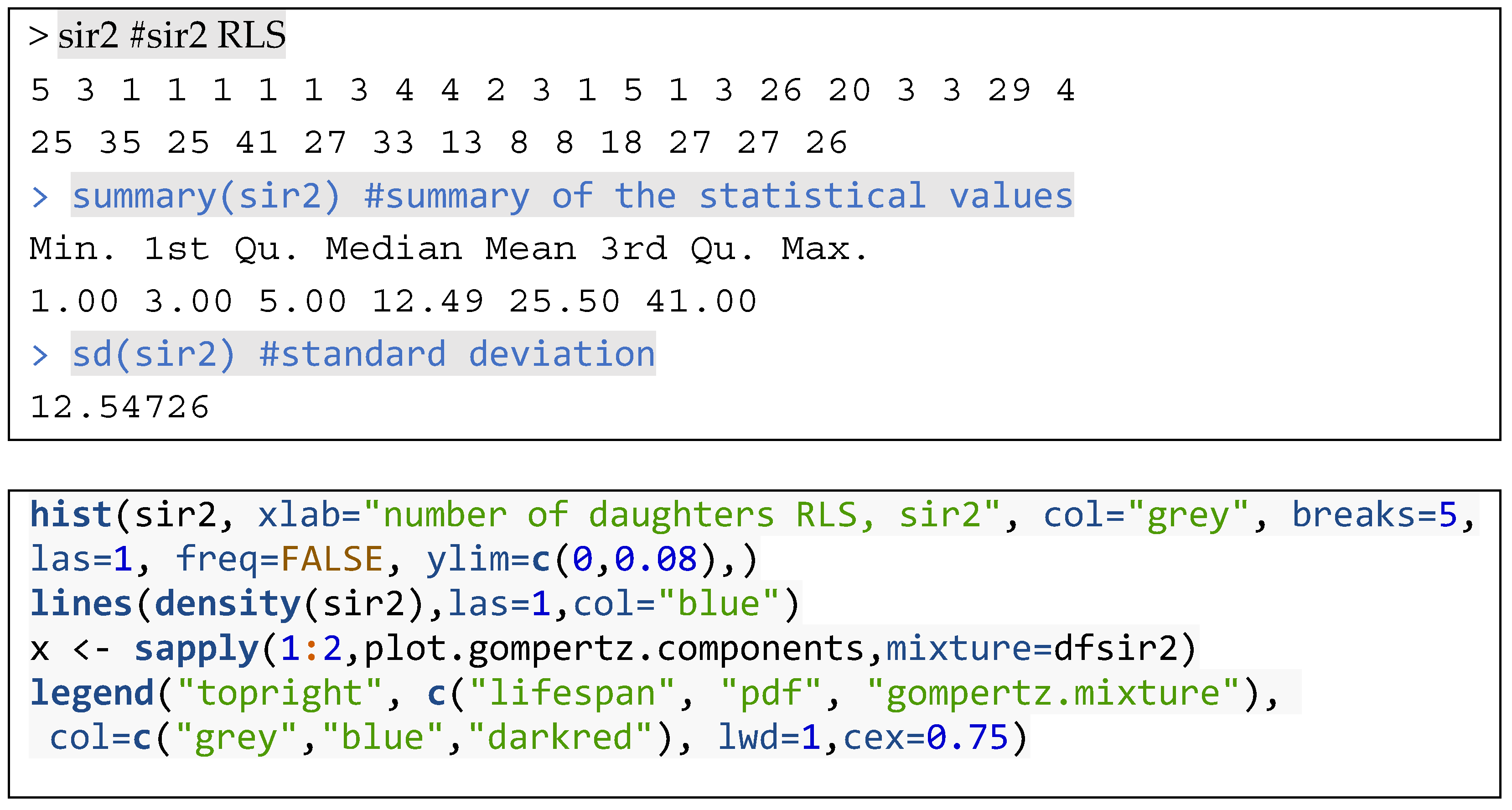
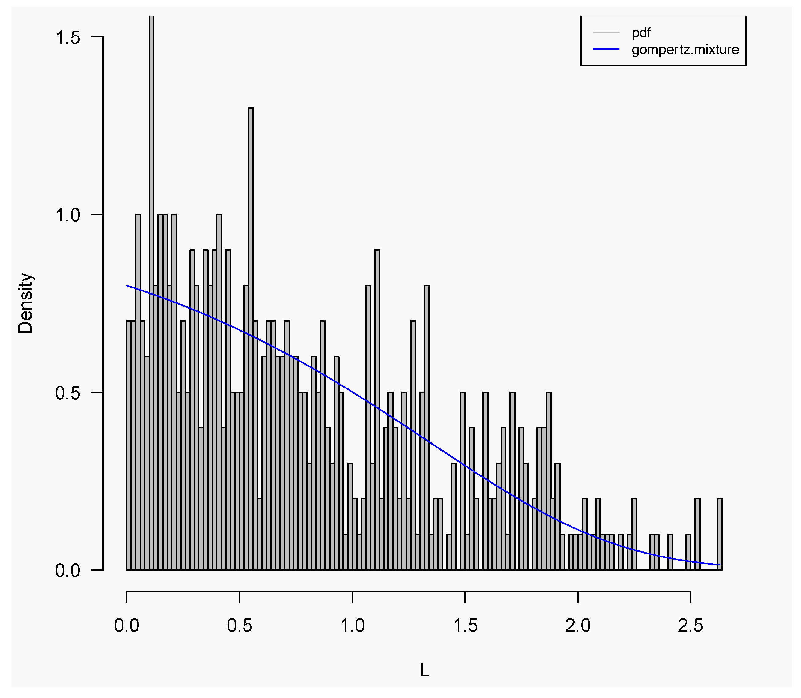
3.1. Working Examples: Fitting Finite Mixture Models to Lifespan Datasets

The fitmixEM function fits lifespan datasets (in the case of yeast cells, this would be the replicative lifespan of a given genetic background) utilizing a finite mixture model in the form of fitmixEM (lifespan, model, $\mathsf{\kappa }$, initial = FALSE, starts)

The lifespan argument denotes genotype backgrounds, strains, or single-gene-deletion strains of lifespan data of dividing cells in the context of RLS; otherwise, it can represent survival time until death, failure, divorce, or relapse. The initial argument depends on the choice of the user, either FALSE or TRUE. If the argument is assigned to FALSE, a value would not set for the starts argument by default. The user must define a vector of (ω, α, β) starting values, which should be assigned to starts. The three-length vector is of $\mathsf{\kappa }=1, \cdots ,\mathrm{g}$number of parameters of a given mixture model with the parts weight ${\mathsf{\omega }}_{\mathsf{\kappa }}$ of the $\mathsf{\kappa }\mathrm{th}$ component, ${\mathsf{\alpha }}_{\mathsf{\kappa }}$ shape, and ${\mathsf{\beta }}_{\mathsf{\kappa }}$ scale or rate parameters of a specified model argument of the $\mathsf{\kappa }\mathrm{th}$ component when initial is set to TRUE.

As is previously employed in the other probability density functions (PDFs) in R studio, the first output is a vector called estimate that includes the estimated parameters of the finite mixture model (weight, alpha, beta) which correspond to weight, shape, and scale parameters, respectively. The second unit (i.e., measures) includes Akaike Information Criterion (AIC), Bayesian Information Criterion (BIC), Kolmogorov–Smirnov (KS), and log-likelihood (log.likelihood) statistics of four goodness-of-fit measures. Finally, the third unit (i.e., cluster) is the clustering employed by the k-means clustering method. As a demonstration, the code below estimates sir2, single-gene deletion mutant replicative lifespan from a two-parameter “Gompertz” mixture model, and presents the distribution of lifespan in Figure 1. The mutant sir2 genetic background has “MATalpha” mating type, media as “YPD” reference single deletion mutants under the temperature 30 °C. Relevant descriptive statistical measurements are as the following:

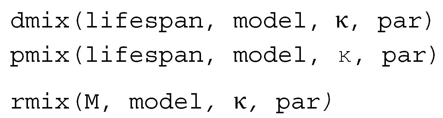
3.2. Distribution Functions for Finite Mixture Models

Similar to classic survival functions in R studio for studying standard probability distributions, we present functions for the computation of the density function dmix, distribution function pmix, and randomly generated rmix vector of values of the finite mixture distributions utilized in fitmix package. The mixture functions presented in fitmix are in the following forms:

where lifespan is a vector of samples (realizations). The model argument is a character string available as PDFs of Gompertz (“gompertz”), Log-logistic (“Log-logistic “), Log-normal (“Log-normal”), and Weibull (“weibull”) models indicating the distributions which are employed to fit lifespan data. M is the number of entries to be simulated for the mixture random generation from the model of the finite mixture, $\mathrm{p}$ is a positive real number that meets $0<\mathrm{p}<1$, $\mathsf{\kappa }$ is the number of parameters of a given model, and $\mathrm{par}$is the parameter vector for finite mixture model that carries the same shape as the argument starts of the fitmixEM function. $\mathsf{\kappa }$ is a sole integer value representing the number of unknown parameters of a given PDF to contain in the model of the finite mixture. Models of the finite mixture parameters are gauged utilizing the Expectation–Maximization (EM) algorithm. As a demonstration, the script below outputs 500 observations from a two-parameter mixture model of Gompertz and demonstrates the results in Figure 2.

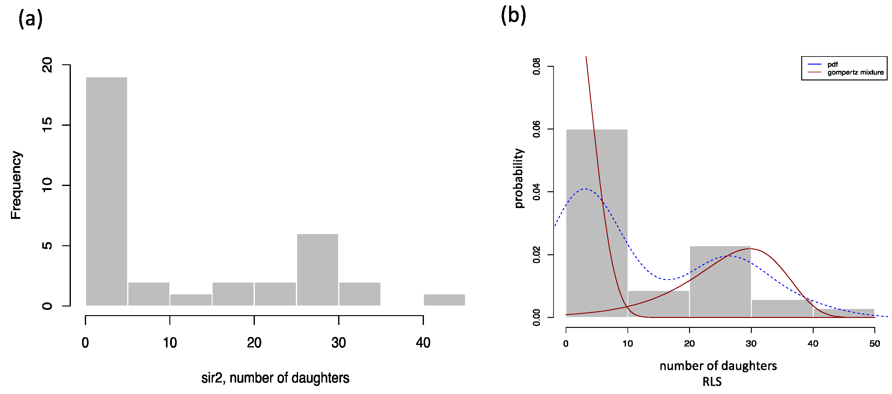
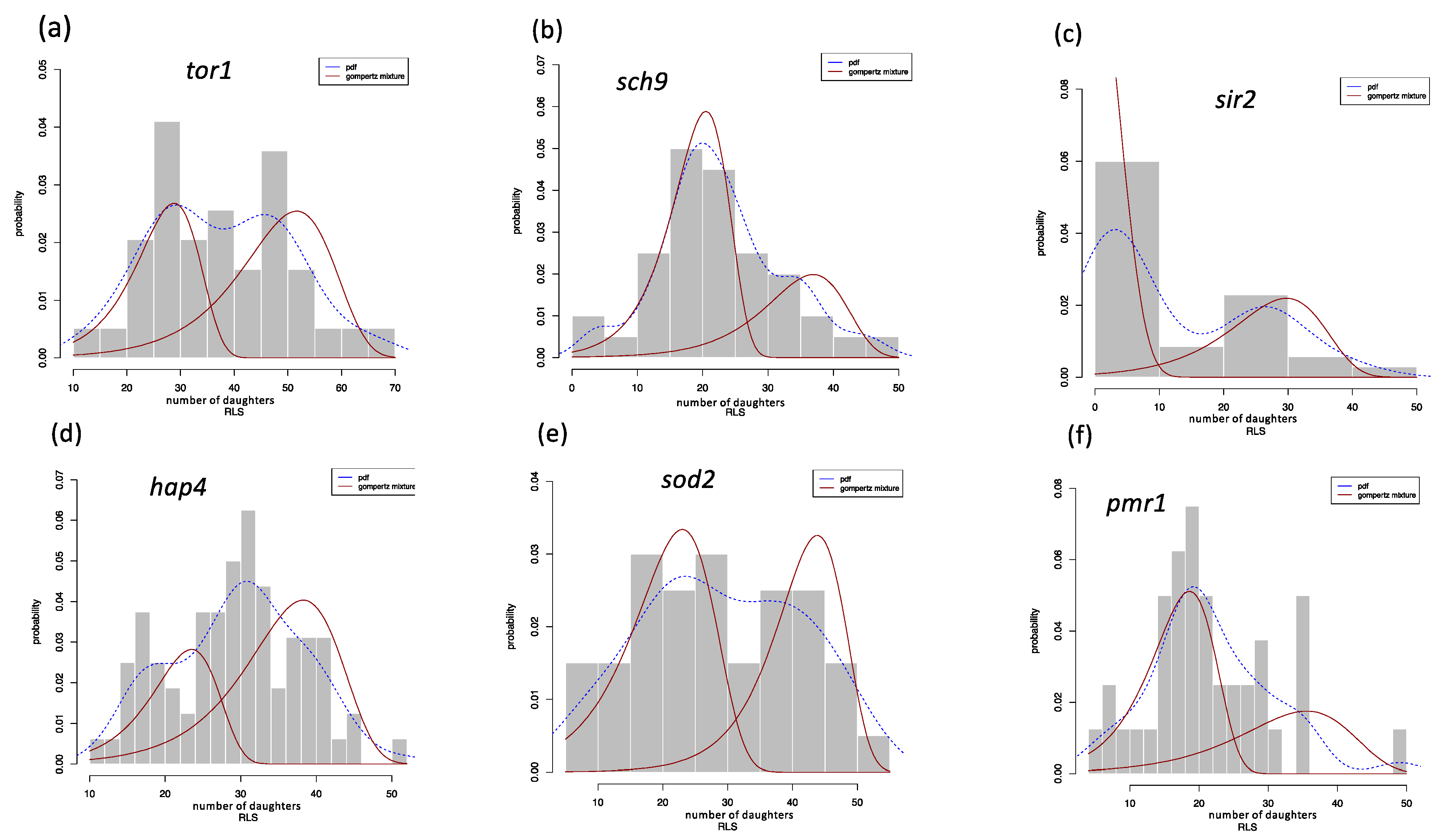
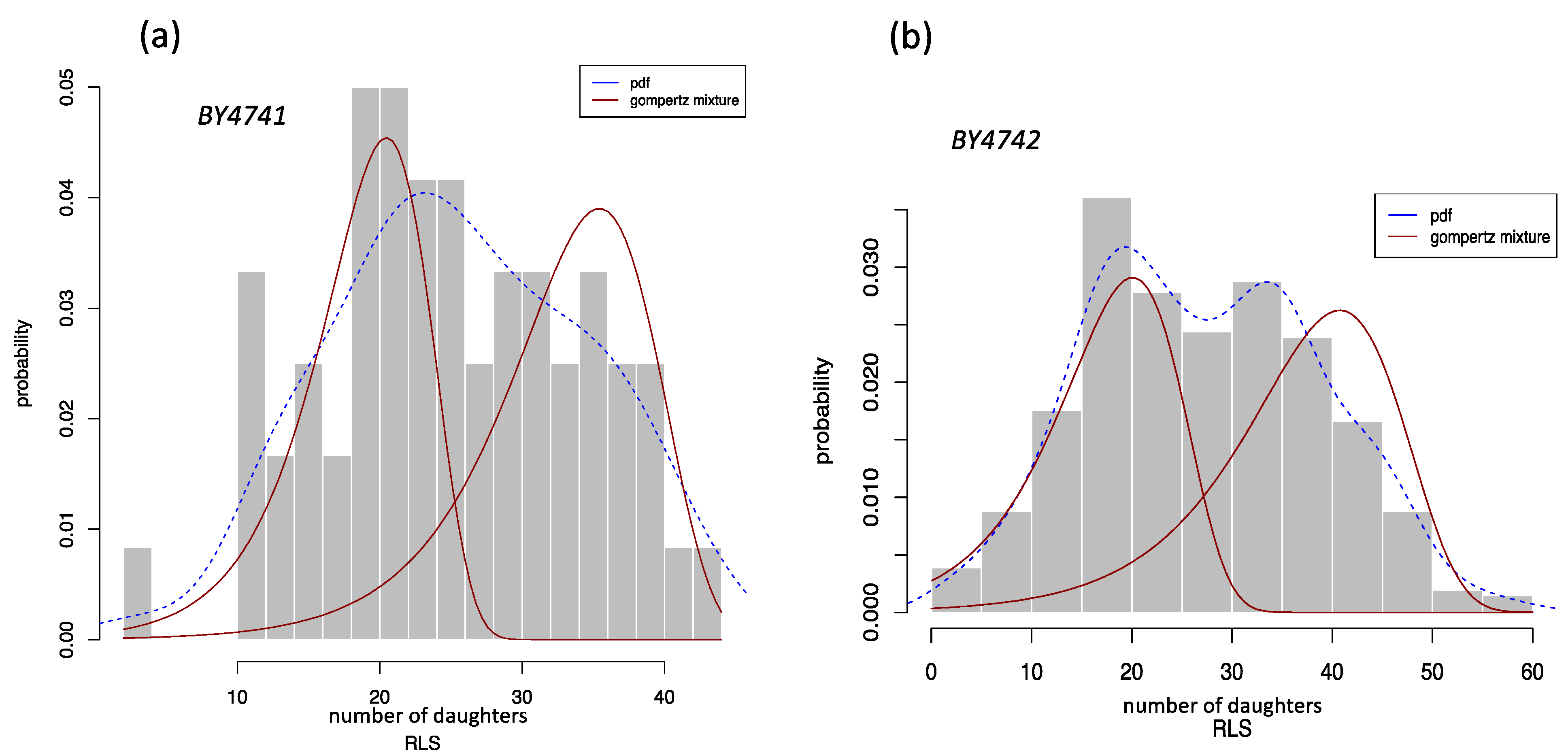
3.3. Finite Gompertz Mixture Model: Yeast Mutants with Known Effects on RLS Application

To better demonstrate the usefulness of the fitmix package, we performed Gompertz mixture model on experimental RLS measurements of single gene deletion mutants with known effects on aging [17,30]. We estimated parameters of the Gompertz mixture model from RLSs of different yeast mutants shown in Figure 3. Since the Gompertz model is a good fit for lifespan data [9,31], such as for deletion mutants tor1, sch9, sir2, hap4, sod2, and pmr1, the fitmix package is even better because it uses the Gompertz mixture model to portray lifespan data.

In Li et al. 2020, two subpopulations were reported during replicative aging. In BY4741 wildtype genetic background, cells have two approximately equally weighted subpopulations. In two single-gene deletion mutants, sir2-deletion and hap4-deletion, the subpopulations are skewed to one subpopulation over another [32]. Our mixture fitting results confirm these significant findings. Based on its histogram, even hap4-deletion may have three subpopulations of cells (

Table 1. Estimated parameters of the finite Gompertz mixture model using the fitmix package.

		Estimated	Parameters
deletion mutants	${\mathsf{\omega }}_1$	${\mathsf{\alpha }}_1$	${\mathsf{\beta }}_1$	${\mathsf{\omega }}_2$	${\mathsf{\alpha }}_2$	${\mathsf{\beta }}_2$
tor1	0.58193	0.11853	0.00025	0.41806	0.17316	0.00118
sch9	0.32569	0.16519	0.00037	0.67430	0.23548	0.00188
sir2	0.41763	0.14042	0.00215	0.58236	0.15148	0.22705
hap4	0.32934	0.23195	0.00099	0.67065	0.16322	0.00031
sod2	0.49874	0.17351	0.0001	0.50125	0.17925	0.00353
pmr1	0.37274	0.12604	0.00142	0.62725	0.22176	0.00377
wildtypes	${\mathsf{\omega }}_1$	${\mathsf{\alpha }}_1$	${\mathsf{\beta }}_1$	${\mathsf{\omega }}_2$	${\mathsf{\alpha }}_2$	${\mathsf{\beta }}_2$
BY4741	0.57262	0.22899	0.00139	0.42737	0.21757	0.00007
BY4742	0.48798	0.17110	0.00443	0.512012	0.13422	0.00053

and Figure 4).

Based on the estimated parameters in Table 1 and using Equations (13) and (15), we obtain the probability density functions and survival functions of the Gompertz mixture distributions as illustrated in Figure 3 and Figure 4. In our analysis, tor1, sir2, and sod2 mutants have RLS that can be fit into two subpopulations. Table 1 demonstrates scg9, hap4, and pmr1 mutants can even be fitted into three subpopulations.

Estimated model parameters of single-mode Gompertz aging model for shape parameter $\mathsf{\alpha }$ ranged between 0.05 and 0.25, rate parameter $\mathsf{\beta }$ranged between 0.0001 and 0.04, which supports that our mixture parameters are correctly estimated by the previous studies [9,14]. We can deduce that the Gompertz mixture model method provides the best fit for the RLS of budding yeast. This agrees with our assumption that a mixture model may be biologically meaningful.

4. Discussion

A common task in yeast aging studies is modeling the lifespan distribution. In this study, we have developed and introduced an R package called fitmix that provides several models and estimation techniques for modeling replicative lifespan distributions from both individual lifespan data and grouped lifespan data, as well as providing additional functionality for simulating finite mixture distributions and fitting curves to division-probability of the data. In our analysis, we show that RLS in many mutants, such as tor1, sch9, sir2, hap4, sod2, pmr1, can be fit into two subpopulations, some of them even three subpopulations. Our study suggests replicative aging in these probably have at least two subpopulations in the other mutants as well (Supplementary Materials), and we argue that these are promising biological insights or hypotheses that may be pursued by experimental biologists. Since experimental studies are expensive and time-consuming, our mixture-modeling approach provides a reasonable alternative research method to assess the aging process in many more yeast mutants.

To help facilitate the comparison of the different model estimation methods provided by the fitmix, we include multiple goodness-of-fit measures that the user can determine the best model technique for their purposes. The fitmix package employs the EM algorithm that might have some other alternatives. However, from the previous section, we can see that simply evaluating Equation (22) to find such parameters would be very hard. An analytical approach to the estimation of parameters requires an explicit formula for the maximum likelihood investigation [33]. Fortunately, there is an iterative method we can use to achieve this purpose. It is called the Expectation–Maximization, or simply EM algorithm [34,35]. It is widely used for optimization problems where the objective function has complexities such as the one that has been encountered in the fitmix package. To avoid converging to a local maximum of the observed data likelihood function, we compare our estimated mixture parameters depending on starting values previously reported [9,14,31].

While this package was developed in the context of yeast research, the models we fit and simulate have numerous applications throughout other biological and medical fields, such as cancer survival data, disease datasets, and lifespan datasets of single units. For example, a similar model of a mixture of a Weibull component and a surviving fraction in the context of a lung cancer trial is considered [36,37,38] and finite mixture distributions are broadly applied in medical and survival statistics (for numerous examples, see [18,39]).

The fitmix package is open-source software released under a GPL3 license on CRAN.

As future work, we think of some software functionality ideas that include: (1) an expanded set of the finite mixture models, particularly the binomial aging model outlined in Qin et al. (2019) and Jackson et al. (2016) [9,40]; (2) a function that automates plots and illustrates survival datasets fitted by mixture models; (3) expansion of user-detected goodness-of-fit measures, including a comparison to the best-fit model; and (4) addition of a Gaussian noise effect [14] that accommodates grouped distribution and replicative lifespan data of the budding yeast, e.g., stands, wildtype strains, single-gene mutant deleted genes.

Another study that could be conducted is examining distinct mixture models to model heterogeneous lifetime data, particularly RLS data. A mixture of Gompertz distributions, a mixture of Log-logistic distributions, a mixture of Log-normal distributions, and a mixture of Weibull distributions would be tested for the best fit to the experimental and simulated survival datasets. The comparisons of theoretical statistical distributions and mixture distribution models for lifetime and survival datasets would be studied in the future.

References

1. Breitenbach, M.; Jazwinski, S.M.; Laun, P. Aging Research in Yeast; Springer Science & Business Media: Berlin, Germany, 2011; Volume 57, ISBN 94-007-2561-2. [Google Scholar]
2. Longo, V.D.; Shadel, G.S.; Kaeberlein, M.; Kennedy, B. Replicative and Chronological Aging in Saccharomyces Cerevisiae. Cell Metab. 2012, 16, 18–31. [Google Scholar] [CrossRef] [Green Version]
3. Spivey, E.C.; Jones, S.K.; Rybarski, J.R.; Saifuddin, F.A.; Finkelstein, I.J. An Aging-Independent Replicative Lifespan in a Symmetrically Dividing Eukaryote. eLife 2017, 6, e20340. [Google Scholar] [CrossRef]
4. Kaeberlein, M. Lessons on Longevity from Budding Yeast. Nature 2010, 464, 513–519. [Google Scholar] [CrossRef] [Green Version]
5. Powers, R.W.; Kaeberlein, M.; Caldwell, S.D.; Kennedy, B.K.; Fields, S. Extension of Chronological Life Span in Yeast by Decreased TOR Pathway Signaling. Genes Dev. 2006, 20, 174–184. [Google Scholar] [CrossRef] [Green Version]
6. Henderson, K.A.; Hughes, A.L.; Gottschling, D.E. Mother-Daughter Asymmetry of PH Underlies Aging and Rejuvenation in Yeast. Elife 2014, 3, e03504. [Google Scholar] [CrossRef]
7. Minois, N.; Frajnt, M.; Wilson, C.; Vaupel, J. Advances in Measuring Lifespan in the Yeast Saccharomyces Cerevisiae. Proc. Natl. Acad. Sci. USA 2005, 102, 402–406. [Google Scholar] [CrossRef] [Green Version]
8. Juckett, D.; Rosenberg, B. Comparison of the Gompertz and Weibull Functions as Descriptors for Human Mortality Distributions and Their Intersections. Mech. Ageing Dev. 1993, 69, 1–31. [Google Scholar] [CrossRef]
9. Qin, H. Estimating Network Changes from Lifespan Measurements Using a Parsimonious Gene Network Model of Cellular Aging. BMC Bioinform. 2019, 20, 599. [Google Scholar] [CrossRef]
10. Jin, M.; Li, Y.; O’Laughlin, R.; Bittihn, P.; Pillus, L.; Tsimring, L.S.; Hasty, J.; Hao, N. Divergent Aging of Isogenic Yeast Cells Revealed through Single-Cell Phenotypic Dynamics. Cell Syst. 2019, 8, 242–253.e3. [Google Scholar] [CrossRef] [Green Version]
11. O’Laughlin, R.; Jin, M.; Li, Y.; Pillus, L.; Tsimring, L.S.; Hasty, J.; Hao, N. Advances in Quantitative Biology Methods for Studying Replicative Aging in Saccharomyces Cerevisiae. Transl. Med. Aging 2020, 4, 151–160. [Google Scholar] [CrossRef] [PubMed]
12. Moustafa, H.M.; Ramadan, S.G. On MLE of a Nonlinear Discriminant Function from a Mixture of Two Gompertz Distributions Based on Small Sample Size. J. Stat. Comput. Simul. 2003, 73, 867–885. [Google Scholar] [CrossRef]
13. Wilkinson, D.J. Stochastic Modelling for Quantitative Description of Heterogeneous Biological Systems. Nat. Rev. Genet. 2009, 10, 122–133. [Google Scholar] [CrossRef]
14. Güven, E.; Akçay, S.; Qin, H. The Effect of Gaussian Noise on Maximum Likelihood Fitting of Gompertz and Weibull Mortality Models with Yeast Lifespan Data. Exp. Aging Res. 2019, 45, 167–179. [Google Scholar] [CrossRef]
15. Everitt, B.S. Finite Mixture Distributions. In Encyclopedia of Statistics in Behavioral Science; American Cancer Society: Atlanta, GA, USA, 2005; ISBN 978-0-470-01319-9. [Google Scholar]
16. McLachlan, G.J.; Lee, S.X.; Rathnayake, S.I. Finite Mixture Models. Annu. Rev. Stat. Its Appl. 2019, 6, 355–378. [Google Scholar] [CrossRef]
17. Saka, K.; Ide, S.; Ganley, A.R.; Kobayashi, T. Cellular Senescence in Yeast Is Regulated by RDNA Noncoding Transcription. Curr. Biol. 2013, 23, 1794–1798. [Google Scholar] [CrossRef] [PubMed] [Green Version]
18. Marín, J.M.; Rodriguez-Bernal, M.; Wiper, M.P. Using Weibull Mixture Distributions to Model Heterogeneous Survival Data. Commun. Stat. Simul. Comput. 2005, 34, 673–684. [Google Scholar] [CrossRef] [Green Version]
19. Tsionas, E.G. Bayesian Analysis of Finite Mixtures of Weibull Distributions. Commun. Stat. Theory Methods 2002, 31, 37–48. [Google Scholar] [CrossRef]
20. Al-Hussaini, E.K.; Al-Dayian, G.R.; Adham, S.A. On Finite Mixture of Two-Component Gompertz Lifetime Model. J. Stat. Comput. Simul. 2000, 67, 20–67. [Google Scholar] [CrossRef]
21. Güven, E. A Comparison between the Performance of Weibull and Log-Logistic Aging Models on Saccharomyces Cerevisiae Lifespan Data. Bilecik Şeyh Edebali Üniversitesi Fen Bilimleri Derg. 2020, 7, 123–132. [Google Scholar] [CrossRef]
22. Blischke, W.R.; Murthy, D.P. Reliability: Modeling, Prediction, and Optimization; John Wiley & Sons: Hoboken, NJ, USA, 2011; Volume 767, ISBN 1-118-15047-3. [Google Scholar]
23. Peel, D.; McLachlan, G.J. Robust Mixture Modelling Using the t Distribution. Stat. Comput. 2000, 10, 339–348. [Google Scholar] [CrossRef]
24. Wilson, D.L. The analysis of survival (mortality) data: Fitting Gompertz, Weibull, and logistic functions. Mech. Ageing Dev. 1994, 74, 15–33. [Google Scholar] [CrossRef]
25. McLachlan, G.J.; Krishnan, T.; Ng, S.K. The EM Algorithm. 2004. Available online: https://www.econstor.eu/bitstream/10419/22198/1/24_tk_gm_skn.pdf (accessed on 18 March 2021).
26. Akaike, H. A New Look at the Statistical Model Identification. IEEE Trans. Autom. Control 1974, 19, 716–723. [Google Scholar] [CrossRef]
27. Schwarz, G. Estimating the Dimension of a Model. Ann. Stat. 1978, 6, 461–464. [Google Scholar] [CrossRef]
28. Smirnov, N. Table for Estimating the Goodness of Fit of Empirical Distributions. Ann. Math. Stat. 1948, 19, 279–281. [Google Scholar] [CrossRef]
29. Fisher, R.A. Two New Properties of Mathematical Likelihood. Proc. R. Soc. London. Ser. A Math. Phys. Sci. 1934, 144, 285–307. [Google Scholar]
30. Kaeberlein, M.; Kirkland, K.T.; Fields, S.; Kennedy, B.K. Sir2-Independent Life Span Extension by Calorie Restriction in Yeast. PLoS Biol. 2004, 2, e296. [Google Scholar] [CrossRef]
31. Qin, H. A Network Model for Cellular Aging. arXiv 2013, arXiv:1305.5784. [Google Scholar]
32. Li, Y.; Jiang, Y.; Paxman, J.; O’Laughlin, R.; Klepin, S.; Zhu, Y.; Pillus, L.; Tsimring, L.S.; Hasty, J.; Hao, N. A Programmable Fate Decision Landscape Underlies Single-Cell Aging in Yeast. Science 2020, 369, 325–329. [Google Scholar] [CrossRef]
33. El-Gohary, A.; Alshamrani, A.; Al-Otaibi, A.N. The Generalized Gompertz Distribution. Appl. Math. Model. 2013, 37, 13–24. [Google Scholar] [CrossRef] [Green Version]
34. Jansen, R. Maximum Likelihood in a Generalized Linear Finite Mixture Model by Using the EM Algorithm. Biometrics 1993, 49, 227–231. [Google Scholar] [CrossRef]
35. Benaglia, T.; Chauveau, D.; Hunter, D.; Young, D. Mixtools: An R Package for Analyzing Finite Mixture Models. J. Stat. Softw. 2009, 32, 1–29. [Google Scholar] [CrossRef] [Green Version]
36. Erisoglu, U.; Erisoglu, M.; Erol, H. MIXTURE MODEL APPROACH TO THE ANALYSIS OF HETEROGENEOUS SURVIVAL DATA. Pak. J. Stat. 2012, 28, 115–130. [Google Scholar]
37. Karakoca, A.; Erisoglu, U.; Erisoglu, M. A Comparison of the Parameter Estimation Methods for Bimodal Mixture Weibull Distribution with Complete Data. J. Appl. Stat. 2015, 42, 1472–1489. [Google Scholar] [CrossRef]
38. Erişoğlu, Ü.; Erişoğlu, M.; Erol, H. A Mixture Model of Two Different Distributions Approach to the Analysis of Heterogeneous Survival Data. Int. J. Comput. Math. Sci. 2011, 5, 75–79. [Google Scholar]
39. Morin, A.J.S.; Litalien, D. Mixture Modeling for Lifespan Developmental Research. Available online: https://oxfordre.com/psychology/view/10.1093/acrefore/9780190236557.001.0001/acrefore-9780190236557-e-364 (accessed on 13 April 2021).
40. Jackson, C. Flexsurv: A Platform for Parametric Survival Modeling in R. J. Stat. Softw. 2016, 70, 1–33. [Google Scholar] [CrossRef] [PubMed] [Green Version]
Figure 1. (a) Number of daughters (RLS) and frequency histogram of the sir2 deletion genetic background is illustrated. (b) The histogram of number of daughters (RLS) of sir2 from a two-component Gompertz model is shown.
Applsci 11 06114 g001
Figure 2. Histogram plot of 500 randomly distributed realizations from a two-parameter mixture model of Gompertz.
Applsci 11 06114 g002
Figure 3. Overlay of Gompertz mixture fitting curves with RLS histograms in yeast mutants. Red fitting curves represent the Gompertz mixture fit to the RLS data of yeast mutants, and the probability density functions of lifespan data are represented with the blue dashed fitting curves; (a) tor1, (b) sch9, (c) sir2 and (d) hap4, (e) sod2, (f) pmr1.
Applsci 11 06114 g003
Figure 4. Overlay of Gompertz mixture fitting curves with RLS histograms using experimental replicative lifespan datasets for the laboratory (a) BY4741 and (b) BY4742 wildtype reference strains. Red fitting curves represent the Gompertz mixture fit to the RLS data of (a) BY4741 and (b) BY4742, and the probability density functions of lifespan data are represented with the blue dashed fitting curves. See Table 1 for estimated parameters of the finite Gompertz mixture fits.
Applsci 11 06114 g004