Automatic Handgun Detection with Deep Learning in Video Surveillance Images

Abstract

There is a great need to implement preventive mechanisms against shootings and terrorist acts in public spaces with a large influx of people. While surveillance cameras have become common, the need for monitoring 24/7 and real-time response requires automatic detection methods. This paper presents a study based on three convolutional neural network (CNN) models applied to the automatic detection of handguns in video surveillance images. It aims to investigate the reduction of false positives by including pose information associated with the way the handguns are held in the images belonging to the training dataset. The results highlighted the best average precision (96.36%) and recall (97.23%) obtained by RetinaNet fine-tuned with the unfrozen ResNet-50 backbone and the best precision (96.23%) and F1 score values (93.36%) obtained by YOLOv3 when it was trained on the dataset including pose information. This last architecture was the only one that showed a consistent improvement—around 2%—when pose information was expressly considered during training.

1. Introduction

According to data collected in 2017 and published by the Small Arms Survey [1], the percentage of firearms held by civilian worldwide was approximately 85% compared to the 13% held by the army forces and 2% by law enforcement (see Figure 1). By country, the number for the USA stands out with a total of 393,347 firearms—most of them unregistered—for a total population of 326,474 inhabitants, representing 120.5 firearms per 100 inhabitants and meaning that it ranks first in both the total number of firearms possessed by civilians and in number of weapons per 100 inhabitants. Spain, with 7.5 firearms per 100 inhabitants ranks 103 out of the 227 countries included in the aforementioned report. These data together with the increase in terrorist attacks and shootings with civilian casualties in regions that are not under armed conflict have raised the need to establish surveillance mechanisms, especially in public spaces susceptible to a large influx of people [2] such as transport terminals, educational, health, commercial, and leisure facilities, etc.

Surveillance in public spaces takes multiple forms (which can appear in combination):

• CCTV video surveillance;
• Patrol of security agents;
• Scanning luggage through X-rays;
• Active metal detection;
• Individual frisking of people.

Video surveillance is an inexpensive method that allows covering large areas without interfering with the flux of people. However, it faces major limitations such as those arising from image capture speed, image resolution, scene light quality, and occlusions. In addition, the task of monitoring images captured by CCTV systems requires a high level of attention over long periods of time, which leads to unnoticed events because of human operator fatigue.

For a firearm detection system to be efficient, it must have two characteristics:

• Be able to perform real-time detection;
• Have a very low rate of undetected visible weapons (false negative rate (FNR)).

The first of those requirements is determined by the maximum number of frames per second (fps) that the system can process without losing accuracy in detection. The second provides the most critical type of detection failure, when visible weapons in images are undetected by the system.

To propose a system that meets the two characteristics previously noted, this work presents a study of three firearm (handgun) detectors in images based on the application of convolutional neural networks (CNNs). While “classical” methods require the manual selection of discriminant features [3], CNNs are able to automatically extract complex patterns from data [4].

For problems with a low availability of data and/or limited computational resources, the CNN training can be initiated with the parameters (weights) obtained by pretraining the network on a similar problem. This method is called transfer learning. Based on the initial learned values of the network parameters, network training continues with specific examples for the problem under study. When transfer learning techniques span not only the final layer, but all network parameters, this is called fine-tuning. Transfer learning and fine-tuning embrace the intuition that the features learned by CNNs could be shared in similar problems; hence, the models can avoid starting the learning process from scratch for every new problem.

To reduce the number of undetected objects or false negatives (FNs) without increasing the number of incorrect detections (false positives (FPs)), this work aimed made the hypothesis that incorporating pose information associated with the person holding a weapon should improve the performance of the models. By including pose information, the objective is to avoid detection errors due to the small size of handguns in the images, partial occlusion when holding them, and low image quality.

The manuscript is organized as follows. Section 1 presents the motivation for the problem. Section 2 includes a review of related works focused on weapon detection based on computer vision methods, a description of the most important aspects of the architectures used in the study, and the metrics for the assessment of the results. The section also describes pose detection methods and how these can be used in weapon detection. Section 3 explains the methods to obtain the original dataset (without pose information) used for training, validation, and testing of the proposed models. This section ends by describing the process of adjusting models for the detection problem under study and the experiments conducted. Section 4 exposes and comments on the results obtained. Finally, Section 5 summarizes the main aspects of the work and discusses future efforts directed at overcoming the weaknesses and improving the results of the CNN-based models for handgun detection.

2. Related Works

The problem of the automatic detection of firearms and bladed weapons hidden inside luggage has been tackled for some years using images obtained with X-ray scanners. To this end, the classical cascade-based learning techniques of Haar feature detectors and AdaBoost classifiers [5] have been applied. Indeed, those methods can only work with expensive X-ray scanners and cooperative individuals. A very interesting complementary context is the detection of visible weapons in images captured by CCTV systems, since these systems are already common in video surveillance of public spaces and allow detecting weapons held by noncooperative individuals, regardless of the construction material of such weapons.

One of the most important challenges when training learning models that are fed with CCTV images is the scarcity of the data. Some early methods employed learning techniques based on color segmentation followed by point of interest detection in segmented RGB images [6,7]. The more recent work [7] achieved recall values of 94.93% and a false positive rate of 7% for knife detection, while the figures for firearm detection were 35.98% and 3.31%, respectively.

The use of deep learning techniques to solve computer vision problems [8,9,10,11,12] has achieved great popularity in the last decade in comparison with traditional machine learning techniques. This popularity is due to both its excellent results and the lack of necessity for the manual selection of features to solve the problem. These networks are based on adjusting or learning the parameters (weights) during their training using the gradient descent algorithm, which aims to minimize the network’s response error or loss function. In this optimization process, the error is backpropagated through the network to adjust its parameters across all its layers. This process is also known as error backpropagation through the network. The use of convolution operations allows considering the process of adjusting the network weights as that of obtaining filters that focus on the characteristics that solve the problem, even when dealing with heterogeneous datasets [13]. The network depth provides different levels of the abstraction or composition of features associated with the input images.

CNNs are applied with excellent performance in three related computer vision problems:

• Classification [11]: Given an image of a foreground object, the objective is to indicate what is the label or class that identifies that type of object (see the example in Figure 2a);
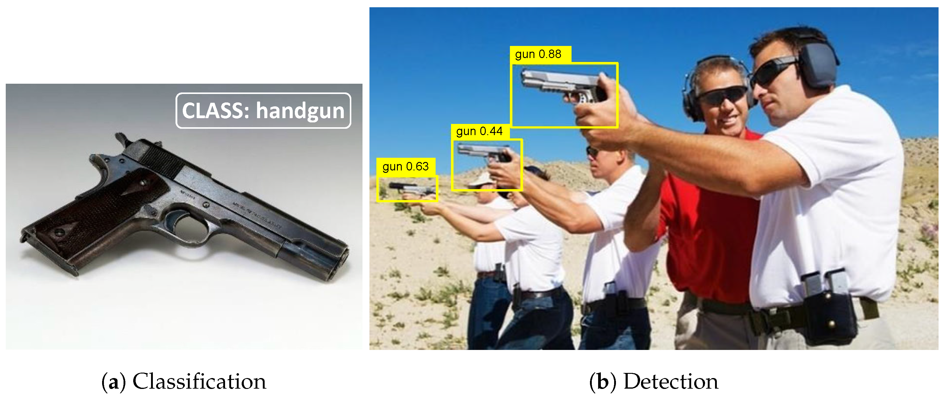
• Detection [8,10]: Given an image with multiple objects present in it, each object must be located by marking in the image the bounding box (bbox) that contains it. A label indicating the type of object contained and a certainty value (between zero and one) for such a prediction is added to each bbox (see the example in Figure 2b). It is common to consider a prediction valid, successful or not, when the prediction’s certainty or confidence score exceeds a threshold value (e.g., 0.5);
• Segmentation: Given an image, each pixel must be labeled with the class of the object to which that pixel belongs.

Before a concise review of the most relevant models based on CNNs for object detection—in general—and firearms’ detection in video images—in particular—the fundamental metrics for the performance assessment of the detection models included in our present study are described.

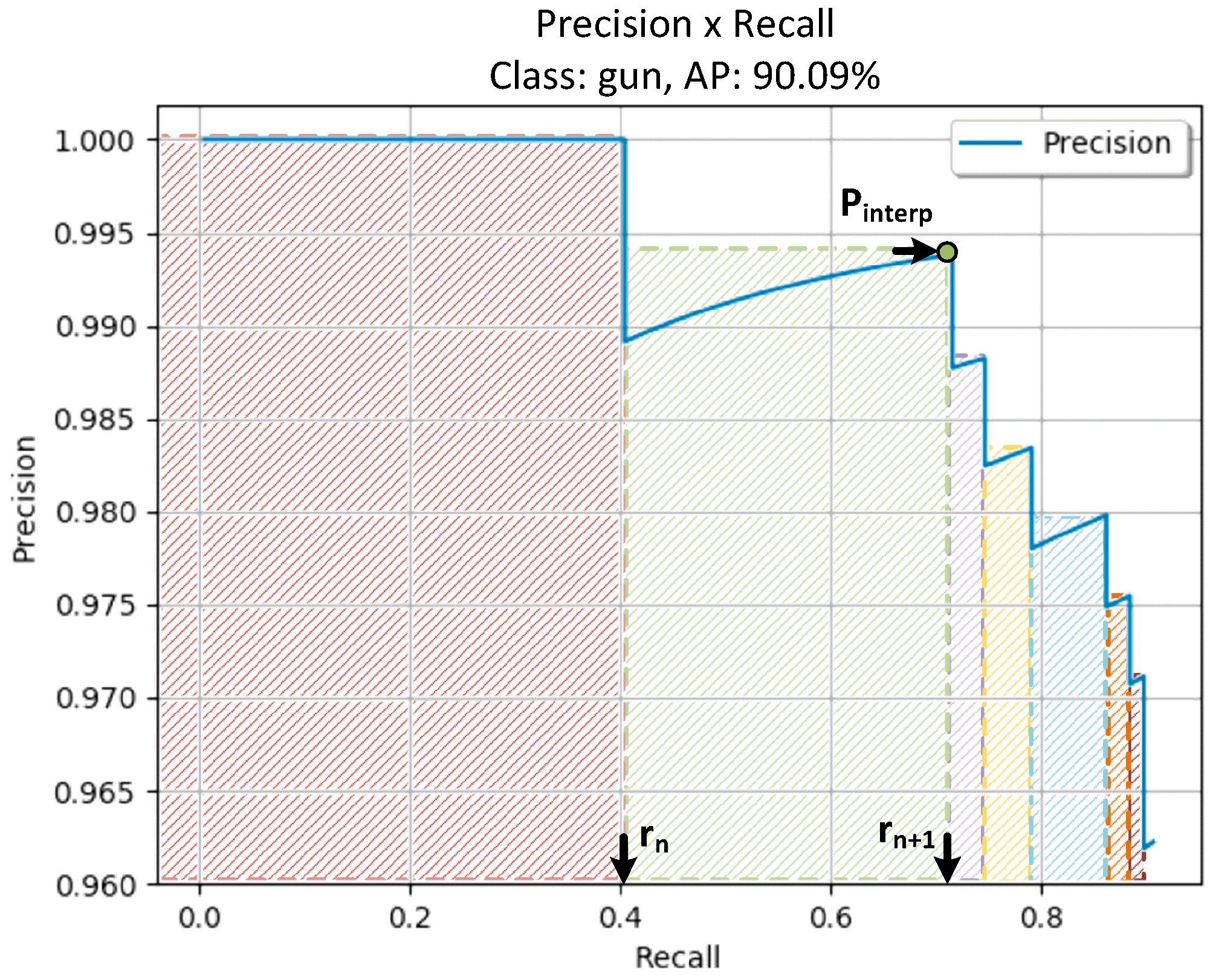
2.1. Performance Metrics

In order to compare the results obtained by the different object detection models included in this study, it is essential to establish a standardized framework that provides the performance metrics on which the comparisons are based. The main way to promote the development of these standardized comparison frameworks has been to conduct competitions that establish common rules to solve a particular problem and measure the quality of the final results achieved with a unique test dataset. The most popular competitions in image-based object detection are:

• The PASCAL VOC Challenge [14];
• The COCO Object Detection Challenge [15];
• The Open Images Challenge [16].

Those competitions used the mean average precision (mAP) as the main metric, considering this as the mean—for all the classes considered in the problem—of the estimated area under the precision × recall curve (PxR curve). To consider the detection of an object as correct (true positive or TP), incorrect (false positive or FP), or undetected (false negative or FN), two values related to the bbox area obtained for each detected object ($B_p$) are considered:

• Confidence score of the detection: This is the value in the range $[0,1]$ obtained by the algorithm, which represents the certainty value of the object’s membership within the box with the indicated class;
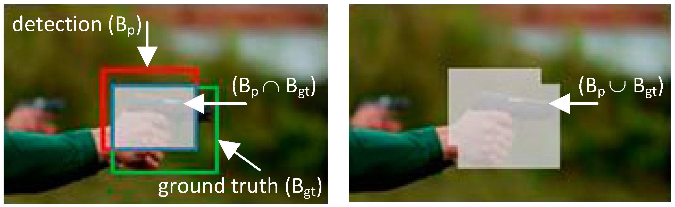
• Intersection over union (IoU): This takes into account the area of the object bbox in the ground truth ($B_{\mathrm{gt}}$) and that of the bbox obtained by the detection algorithm ($B_p$) when both areas overlap. It is calculated as the ratio between the values of the intersection of the areas by the junction of both areas (see Equation (1) and Figure 3). By its own definition, it is a value in the range $[0,1]$.

$$\mathrm{IoU}=\frac{\left(B_{\mathrm{p}}\cap B_{\mathrm{gt}}\right)}{\left(B_{\mathrm{p}}\cup B_{\mathrm{gt}}\right)}$$

(1)

The IoU and confidence score values are used to determine if each detected object is considered a true/false positive (TP/FP). In general, for a detected object to be considered the correct detection (TP), three conditions must be met:

• The confidence score for $B_{\mathrm{p}}$ is greater than a threshold value;
• The class that is predicted for the detected object matches the class included in the ground truth (GT) for that object;
• The IoU value for the detected object exceeds a threshold (usually ≥0.5).

If any of the above criteria is not met, the object is considered an FP (incorrect detection). Some additional rules for determining the TP and FP counts are included in the case of the PASCAL VOC Challenge [14,17]. For example, in the case of multiple detections that correspond to the same object in the GT, this is considered a single TP that corresponds to the $B_{\mathrm{p}}$ with the highest confidence score value, and the rest are considered FPs.

With the total number of TPs and FPs, it is possible to calculate the precision and recall values. They correspond respectively to the proportion of correct detections, or the positive predictive value (PPV), and the ability to correctly detect the positives, or the true positive rate (TPR).

It is important to note that the FN calculation is performed indirectly because as GT_P is the number of positives included in the ground truth, then:

$$\mathrm{GT}\_\mathrm{P} = \left(\mathrm{TP}+\mathrm{FN}\right) \Rightarrow \mathrm{FN} = \left(\mathrm{GT}\_\mathrm{P}-\mathrm{TP}\right)$$

In general, precision and recall vary in opposite directions when the confidence scores change, in such a way that trying to reduce the FP by increasing the precision (i.e., by increasing the confidence score) causes an increment in the number of FNs. Conversely, an increase in the proportion of detected objects in the GT (i.e., by decreasing the confidence score) leads to an increase in the FPs, which reduces the precision value. For this reason, the PxR curve is used to assess the results of a detector, as the detector will be better as long as it maintains a high precision by increasing the recall value. This curve describes how the precision and recall vary for different threshold values chosen for the confidence score of the prediction made by the detector. Since it is difficult to directly compare the values of PxR curves, the so-called average precision (AP) is used as an approximation to the area under the curve, which is calculated by interpolating the curve values [18] according to the equation:

$$\mathrm{AP}=\sum _{n=0}\left(r_{n+1}-r_n\right)·P_{\mathrm{interp}}\left(r_{n+1}\right)$$

(2)

with

$$P_{\mathrm{interp}}\left(r_{n+1}\right)=\underset{\tilde{r}:\tilde{r}⩾r_{n+1}}{max}P\left(\tilde{r}\right)$$

(3)

where $P\left(\tilde{r}\right)$ is the precision at the value of recall $\tilde{r}$. Equation (2) indicates how to compute the area under the PxR curve as the sum of rectangular areas [17]. Each confidence score produces a value pair (precision, recall), for each of these pairs, starting from the highest to the lowest recall values, and the interpolated precision is taken as the highest precision between consecutive recall values (see Equation (3)).

In multiclass detection problems, the AP value is averaged for all classes to obtain the mean average precision value (mAP) as a popular performance metric.

2.2. Two-Stage Detectors

These are also known as classification-based detectors. In the first stage, the candidate areas for the object’s location are obtained. In the second stage, each of the previously obtained candidate areas is entered into a classifier that predicts the type of object (class) contained in that region.

Historically, the concept of a sliding window was firstly used to obtain all possible regions in which the desired object is located, as in the specific case of weapon detection in CCTV images. Although this type of implementation achieves predictions with a great accuracy of nearly 98% [19], these are solutions are not real-time because too many regions need to be analyzed in the image (in the order of thousands) and the required time is too high (14 s/image).

In obtaining promising regions where an object may be located, a major breakthrough was achieved with the R-CNN or region-based CNN [20]. This approach uses the selective search algorithm [21], which then feeds a CNN, which obtains a feature map sent to a support vector machine (SVM) classifier, whose output is the type of object present in each region. Moreover, the right size for the window containing each object is adjusted by regression. This network has been successfully applied in weapon detection applications using image catalogs [22]. However, with a processing time of 49 s/image, this is far from achieving real-time detection.

The Fast R-CNN [23] was an enhancement proposed to decrease the processing time required by the R-CNN. In that approach, the selective search of regions was transferred to the CNN output; hence, the search was performed on the feature map obtained by that network. This reduced the network training time by almost 90% and the inference time by 95% (2.3 s/image). However, the values achieved were still far from real-time processing.

The Faster R-CNN [24] was proposed to achieve the required processing speed for real-time applications. In the Faster R-CNN, the non-learning-based selective search algorithm is substituted by a region proposal network (RPN), which “learns” how to determine regions in which the objects are located. To propose the regions where each object is located, the RPN network slides an $n\times n$ spatial window of the input convolutional feature map obtained by the convolutional layers of a backbone network (e.g., VGG-16). The number of total proposals for each location is k. Therefore, as $k=n\times n$, $n=3\Rightarrow k=9$. The feature map is fed in parallel into two fully connected layers, a regressor (reg), which provides the prediction of the object bbox, and a classifier (cls), which predicts the object class. This architecture allows processing up to 5 fps (i.e., 0.20 s/image). Some of the latest works for detecting firearms via CNN employ this architecture [25,26,27], which is considered the most effective and the fastest in its class, although it is still far from processing 30 fps of video in real time.

In general, two-stage detectors provide high accuracy even in cases with partial objects occluded in images. The accuracy achieved in firearm detection with those detectors reached 84.2% [26]. However, they require significant computing resources and longer training and inference times, and therefore, they are less suitable for applications with limited resources and real-time requirements.

2.3. Single-Stage Detectors

Unlike two-stage detectors, in these architectures, detection is performed in a single step, either on a fixed set of regions in the entire image or a set of feature maps that correspond to multiple image resolutions (to compensate for scale differences). The algorithms predict the class and bbox of the detected objects with a certainty value greater than a threshold value.

Among the most popular of these detectors are: YOLO and its successive improvements [28,29], the single-shot multibox detector [30] (SSD), and RetinaNet [31]. RetinaNet introduced the interesting concept of focal loss, which balances learning the positive object detection and the negative detection for the image background. Bochkovskiy’s work [32], which represented a considerable improvement over YOLO, included a very complete comparison of several detectors in a single stage with real-time inference capability (≥30 $\mathrm{fps}$). These methods have recently been used in several works on automatic firearm detection [33,34,35].

In general, one-stage detectors provide less accuracy than two-stage-based detectors, although they require fewer resources, their architectures are simpler, and they are better suited for real-time applications because of the shorter inference times [36,37].

2.4. Components of Detection Architectures

It is common for object detection frameworks to organize their hierarchical architecture into three components:

• Backbone network: Some of the networks used are Darknet-53, firstly employed for YOLO [28], VGG-16 [38] and ResNet-50/101 [39], which can be used with a setting obtained by training on a dataset elaborated for similar contexts;
• Neck: This is the part of the network that strengthens the results by offering invariance to scale through a network that takes feature maps as the input at different scales. A very common implementation method is the feature pyramid network (FPN) [40] and the multilevel feature pyramid network (MLFPN) [41];
• Detection head: This is the output layer that provides the location prediction of the bbox that delimits each object and the confidence score for a particular class prediction.

2.5. Detection of Weapons and the Associated Pose

While several object detection techniques have been proposed for the detection of firearms in images, some of them are focused on reducing the number of false positives (FPs) without undermining the accuracy or the time required for inference [26,33,42]. However, this endeavor faces a major challenge related to the scarcity of quality datasets to validate the results achieved. The limited quality of existing data is due to various causes such as: the small size of handguns in the images, occlusions by body parts (mainly the hands holding the firearm), poor lighting, low contrast, etc. For this reason, some studies have been conducted to improve the results of detectors by enriching the datasets using contextual examples of CCTV images such as low-quality images [43] and synthetic examples [27].

To tackle the previously noted limitations, one of the aims of our work was to analyze if the individual’s body pose was a useful cue to increase the detection robustness of the handguns in video images. By including pose information, the CNN models learn to detect handguns and the human pose associated with holding them. In this line, Velasco’s work [44] incorporated pose information into a handgun detector to generate a visual rendering using heat maps that combines the representation of the pose and the handgun location. On the contrary, in our work, the pose information obtained through a pose detector was blended with the handgun detector’s training images to study whether CNNs can learn the association of a handgun location with the visual patterns of the pose skeletons included in the training images (see Figure 4).

The scarcity and adequacy of datasets for the detection of handguns in video surveillance images has motivated the development of the dataset in our work. This dataset was constructed with the intention of having quality information to train the detection models in order to analyze the influence of the pose associated with the act of holding a gun. This also allowed validating the blending pose method on the training images. To incorporate pose information into the detection of handguns in 2D images, it was necessary to use a pose detector with the ability to obtain the posture of several people appearing simultaneously in the image in real time (see Figure 4).

The input to the pose detector consisted of an image with one or more individuals in the scene. For each of the subjects, the pose detector computed up to 135 body keypoints whose union represented the skeleton of each person’s posture. OpenPose [45] is one of the most popular pose detectors due to its ability to detect the pose in real time for multiple people simultaneously in the images and the availability of its source code. OpenPose automatically extracts the required features using the first layers of the VGG-19 network [38]. The output of this network is introduced into two subnets to obtain a prediction of the keypoints and their degree of association with the particular skeleton that corresponds to each person present in the image.

3. Materials and Methods

As stated in Section 1, the two main purposes of this work were: (1) the analysis of three object CNN-based detection models applied to handgun detection; and (2) the analysis of the influence of incorporating explicit pose information on the quality of the results of such learning models. For the sake of simplicity, we decided to consider a unique class (“handgun”) as the target of detection to analyze the influence of the pose. For this purpose, two experiments were designed comparing the results for each model with and without pose information during training. Figure 5 shows the system block diagram to provide a whole overview of the method and the data flow in the system.

To consider different detection paradigms (see Section 2 on the related works), the chosen detection architectures and their associated backbone networks were (with reference to their public Keras/TensorFlow implementation used in our experiments):

• The Faster R-CNN with VGG-16 [24,46];
• RetinaNet with ResNet-50 [31,47];
• YOLOv3 with DarkNet-53 [29,48].

The 1220 images that composed the experimental dataset were manually collected from Google Images and YouTube without any automation tool. The process consisted of directly downloading the images from the output results obtained with the Google search engine using keywords and key phrases as the input for the search. The final dataset consisted of the manual selection of images and video frames related to the study context. The selection criteria were:

• The image/frame was not the first plane of a handgun (as in the datasets used in classification problems). Handguns were part of the scene, and they may have had a small size relative to the whole image;
• If possible, the images were representative of true scenes captured by video surveillance systems;
• Images should correspond to situations that guarantee enough generalization capacity for the models; that is, the images covered situations from different perspectives, displaying several people in various poses, even with more than one visible gun;
• Noisy and low-quality images should be avoided. This enhanced the use of fewer data with high-quality information versus the use of more data with low-quality information.

The preparation of the working dataset required the manual assisted annotation of the images that constituted the ground truth (GT) for the models. The annotation process for the images—using the standardized Pascal VOC [14] labeling format—was accomplished with the assistance of the open-source LabelImg program [49]. The annotation process consisted of pointing out the location of the bbox containing the objects to be detected in the image and the identifier of the object class contained in each bbox. In our case, a single “handgun” class was used to simplify the analysis of the results. The input data for training the three chosen models using Keras required a specific input format. This format specification—prepared by customized Python scripts—relied on text files where the essential info was: the image file path, bounding boxes, and class id for the training data.

To perform the desired experiments from the original dataset, a second modified dataset was built with the information associated with the pose obtained by blending the pose skeletons obtained by OpenPose [45] with each original input image (see the block diagram in Figure 5). Both datasets consisted of 1220 images divided into three subsets containing 70%, 15%, and 15% corresponding to training (854 images), validation (183 images), and testing (183 images), respectively. In the experimental models, overfitting during the training process was mitigated by the early stopping callbacks provided by the Keras API. Moreover, the models hyperparameters were set by monitoring—with the tools provided by TensorBoard—the evolution of the loss function for both the training set and the validation set. The three models used in the experiments dealt with the vanishing gradient problem by using the ReLU activation function, which produces bigger derivatives than sigmoids. Furthermore, Keras provides TensorBoard callbacks to diagnose the gradient dynamics of the model during training, such as the average gradient per layer. Figure 6 reveals the software hierarchy used in the experiments, pointing out the main modules.

The influence of the inclusion of pose information in the original dataset was assessed through 8 experiments, training each of the selected models with the original dataset and with the modified dataset including the pose information (with the pose). There was only one class in the dataset, and the total number of objects in the dataset was 225 (i.e., GT_P = 225). To avoid staring from scratch and to cope with the low availability of data, all the experiments started with the models pretrained on the MS COCO dataset [15], composed of 120,000 images with 80 classes among them. Hence, the model fine-tuning started with the parameter values obtained from pretraining.

In all the experiments carried out, fine-tuning on our problem-specific dataset spanned 40 epochs with a batch size of 4. The Adam optimization function with an initial learning rate of 0.001 was applied in all cases. The models were readjusted in two separate experimental rounds: the first one with the original dataset and the second one with the modified dataset including the pose information. For the RetinaNet model, two more additional experiments were performed to compare the effect of fine-tuning with the frozen backbone and when the backbone network was also readjusted (with the unfrozen backbone).

For the performance comparison reached by each model in the experiments, the public implementation of the PASCAL VOC metrics provided in the public toolkit by Padilla et al. [17] was used. These metrics consisted of the calculation of the precision and recall values when different confidence scores were considered. The succession of pairs (precision, recall) provided the PxR curve and the estimation of the average precision (AP) as the area under said curve. That estimation was computed by the addition of every rectangular area by applying Equation (2), as illustrated in Figure 7 for the PxR curve obtained with the YOLOv3 model (with the pose).

4. Results

Several metrics were computed to evaluate each model after the eight scheduled experiments with a test subset of 183 images with a total of 255 guns in them (i.e., GT_P = 255). The values of the metrics for each model are summarized in

Table 1. Assessment metrics obtained in the experiments with a confidence score of 0.5 (except AP).

Exp.	Model	#TP	#FP	#FN	Precision (%)	Recall (%)	F1 (%)	AP (%)
1	Faster R-CNN	194	88	31	68.79	86.22	76.53	81.43
2	Faster R-CNN (with pose)	190	71	35	72.80	84.44	78.19	80.79
3	RetinaNetfz	211	25	16	89.41	92.89	91.54	93.12
4	RetinaNetfz (with pose)	203	29	22	87.50	90.22	88.84	89.71
5	RetinaNetufz	219	35	6	86.22	97.23	91.44	96.36
6	RetinaNetufz (with pose)	210	25	15	89.36	93.33	91.30	92.82
7	YOLOv3	200	11	25	94.79	88.89	91.74	88.49
8	YOLOv3 (with pose)	204	8	21	96.23	90.67	93.36	90.09
[44]	Velasco’s work (with pose)	158	2	39	98.75	80.20	88.51	83.6

. This table shows the number of TPs, FPs, and FNs obtained for a confidence value of 0.5 with the correspondent values of the precision, recall, and F1 score. Finally, the AP value was obtained as the area under the PxR curve as stated by the toolkit developed by Padilla et al. [17].

As mentioned in the previous section, the experimental models were trained in two rounds: (1) with the original dataset; and (2) with the modified dataset by blending the pose skeletons obtained with OpenPose for every input image. The purpose of this procedure was to look for differences in performance, training each model with the two aforementioned datasets. Moreover, two additional experiments were run on the model RetinaNet to analyze the effect of model fine-tuning on the (un)frozen backbone network.

The results in Table 1 show that the AP values obtained by the models trained on our dataset without the pose (exp. 1, 3, 5, and 7) were similar to those obtained by the object detection algorithms that constitute the state-of-the-art. In these experiments, the overall best performing model—with the highest AP value—was RetinaNet fine-tuned with the unfrozen backbone (exp. 5, AP = 96.36%). In contrast, the Faster R-CNN exhibited the lowest AP (exp. 1 and 2). Although YOLOv3 (exp. 7 and 8) produced intermediate AP values (88.49∼90.09%), it was the model that offered the highest precision (94.79∼96.23%) and F1 score (91.74∼93.36%) values.

Figure 8 displays the test results of the RetinaNet model for two randomly chosen images. These results revealed the superior detection capability of the model trained with the unfrozen backbone (Figure 8b) because this model was able to detect an FN, previously undetected handgun (see top row) and discard an FP—previously incorrect detection—(see the bottom row).

The other main objective of the study was to analyze the influence of the inclusion of pose information in the dataset. To accomplish this, a second modified dataset was built, from the original, blending in each image the pose skeletons obtained by OpenPose applied to the input images. This modified dataset allowed training the experimental models on images with pose information. The experimental result showed that the explicit inclusion of pose information using the method previously described slightly worsened the handgun detection for the Faster R-CNN and RetinaNet models, obtaining lower AP values in exp. 2, 4, and 6 than those obtained in the counterparts experiments without the pose. For these two models, the addition of the pose information not only reduced the average precision (AP), but also the recall value because of the increase of the undetected handguns (FNs). This effect may be due to the fact that these models employ architectures that “learn” from the original dataset (without the pose) implicit complex characteristics associated with the pose, so that the blending of the skeletons obtained with OpenPose had an effect analogous to the addition of “noise”, which hinders detection.

A significantly different effect could be observed in the experiments carried out with the YOLOv3 models (exp. 7 and 8). In these experiments, the detection results offered an improvement of 1.6% in the AP value. Moreover, a rise in both precision and recall by 1.44% and 1.78%, respectively, was noticed. These results could indicate that the inclusion of the pose information did not worsen the detection performed by YOLOv3, and it even improved detection. One possible explanation for this fact could be that the YOLOv3 architecture “learns” more localized features in a region and therefore itself is less capable of extracting complex features associated with the pose. However, when the pose adds information to the region in which the object is located, such as fingers, wrist, and forearm, then the object is detected better (i.e., with higher confidence scores). This explanation is consistent with the observations of the results shown in Figure 9.

Figure 9 shows the detection with YOLOv3 in three test images when training was performed first on the original dataset (top row) and then on the dataset with the pose information (bottom row). In the image on the right side, all objects in the ground truth were detected correctly with and without the pose information. However, when the pose was considered, the confidence score values were higher, especially when the detection box contained pixels associated with the pose.

The central top image shows a false positive detection and an undetected handgun (FN) that were correctly detected (central bottom image) when the pose information was included. Finally, in the image on the right, it is shown how the inclusion of the pose (bottom image) allowed detecting the gun that in the raw image without the pose (top image) was undetected (FN).

Table 1 includes the results obtained with the only alternative method that considered the pose information (Velasco’s method [44], described in Section 2). As shown in the table, our method outperformed the results obtained by Velasco’s approach. In the context of our challenging dataset, Velasco’s method was severely affected by failures in pose detection, as when the body was not fully visible.

5. Conclusions

This work presented a study of three CNN-based object detection models (Faster R-CNN, RetinaNet, and YOLOv3)—pretrained on the MS COCO dataset—applied to handgun detection in video surveillance images. The three main objectives of the study were to:

• Compare the performance of the three models;
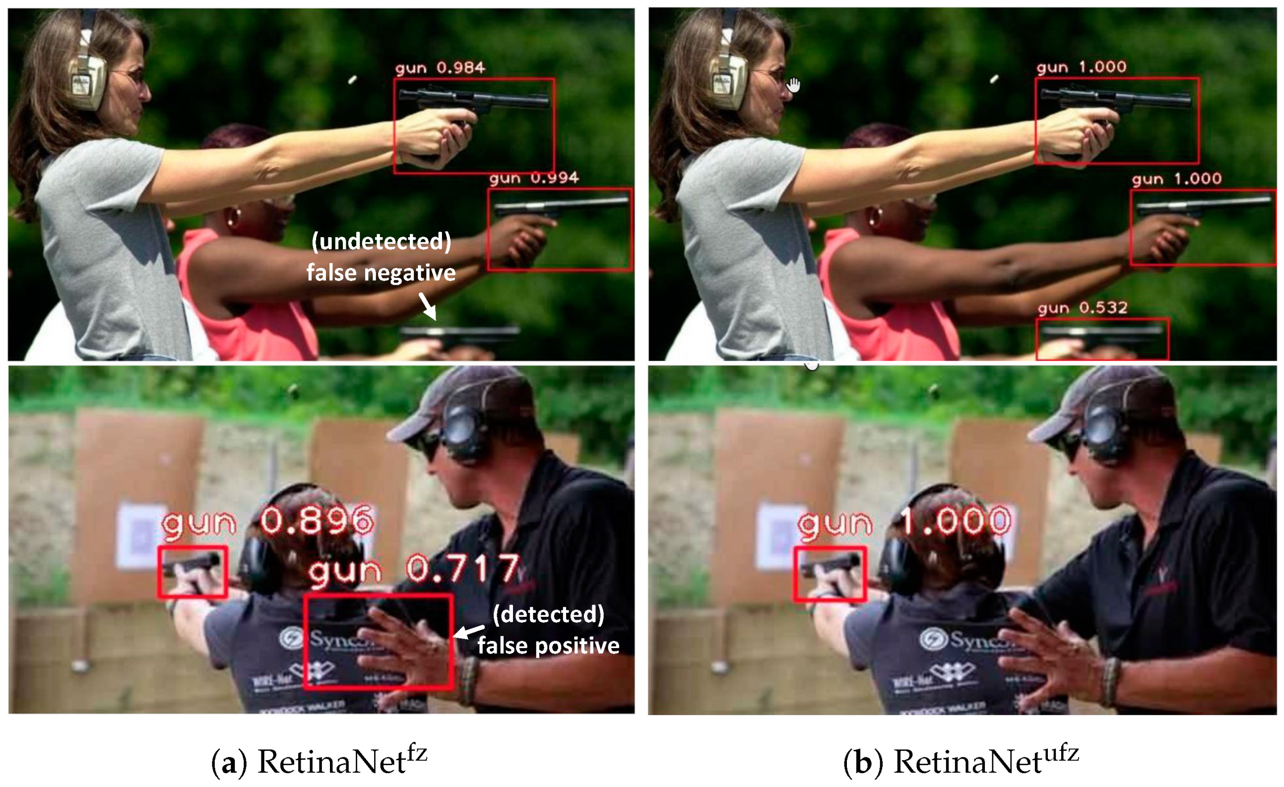
• Analyze the influence of fine-tuning with an unfrozen/frozen backbone network for the RetinaNet model;
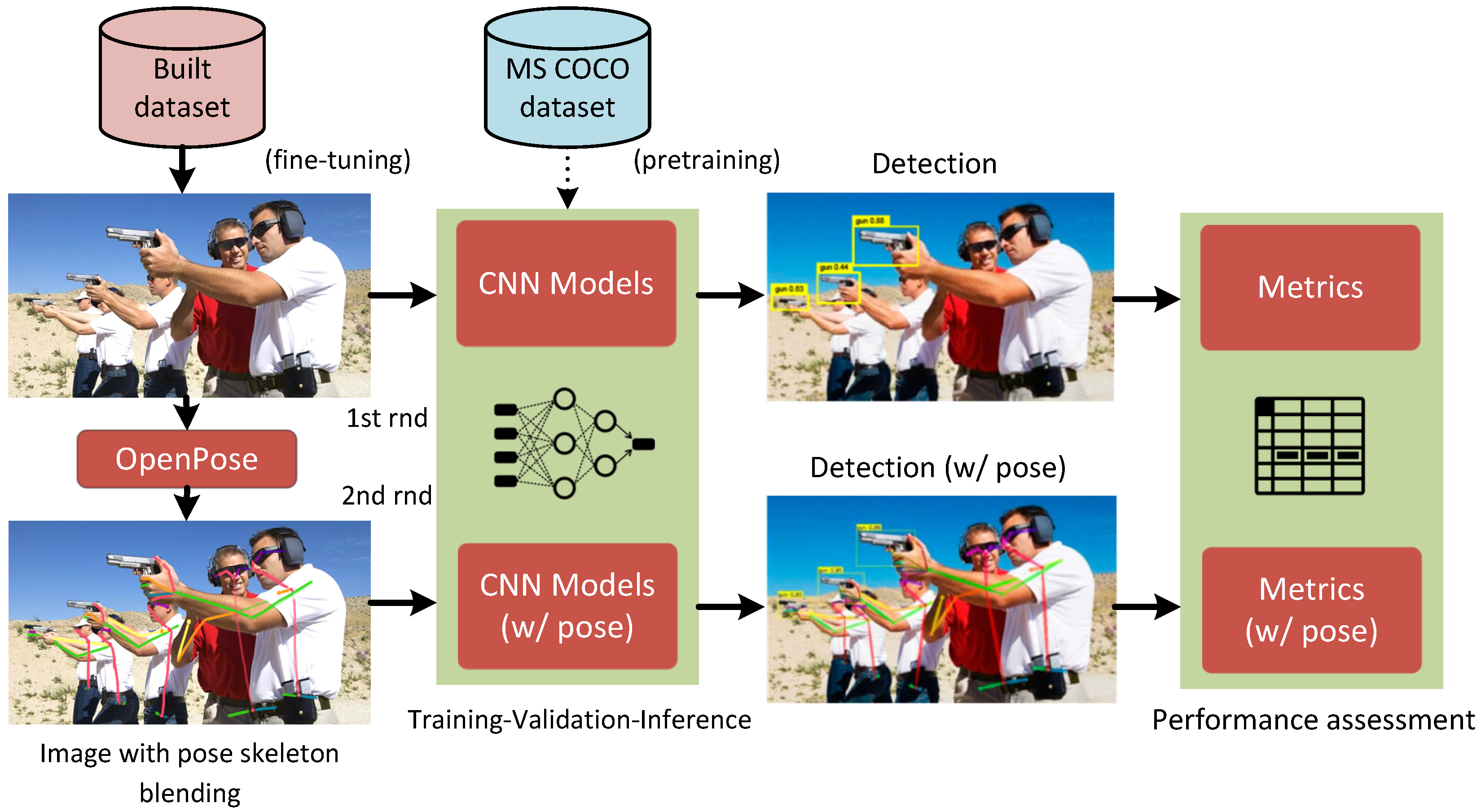
• Analyze the improvement of the detection quality by model training on the dataset with pose information—associated with held handguns—including by a simple method of blending the skeleton poses in the input images.

Using transfer learning by pretraining on the MS COCO dataset, it was possible to obtain the initial values for the experimental models’ parameters, avoiding starting from scratch and overcoming the scarcity of training data. To set the network parameters for the specific detection problem, a dataset composed of 1220 images—with “handgun” as the only target class—was chosen following the selection criterion adapted to the problem.

The assessment of the results in the eight experiments carried out on the 183 test images—unseen during training—was accomplished by comparing, for every model, the standardized metrics (shown in Table 1): precision, recall, F1 score, and average precision (AP) or area under the PxR curve.

The results of the experiments conducted showed that:

• RetinaNet trained by the unfrozen backbone on images without the pose information (exp. 5) obtained the best results in terms of the average precision (96.36%) and recall (97.23%);
• YOLOv3—in Experiments 7 and 8—obtained the best precision (94.79∼96.23%) and F1 score values (91.74∼93.36%);
• The training on images with pose-related information by blending the pose skeletons—generated by OpenPose—in the input images obtained worse detection results for the Faster R-CNN and RetinaNet models (exp. 2, 4, and 6). However, in Experiment 8, YOLOv3 consistently improved every assessment metric by training on images incorporating the explicit pose information (precision ↑ 1.44, recall $\uparrow 1.78$, F1 $\uparrow 1.62$, and AP $\uparrow 1.60$). This promising result encouraged us to further our studies on the ability to improve the way pose information is incorporated into the models;
• When the models were trained on the dataset including the pose information, our method of blending the pose skeletons obtained better results than the previous alternative methods.

RetinaNet and YOLOv3 (exp. 5 and 8) achieved respectively the highest recall (97.23%) and precision values (96.23%). Therefore, it would be desirable in future works to bring together in a single model the positive characteristics of these two architectures. Finally, our results also compared favorably with an alternative method that also considered the pose information.

Considering the specific results from the tests with YOLOv3, some of the false positives detected were found to derive from the inability to distinguish classes of objects similar in size to handguns and held similarly to a handgun (e.g., smartphone, wallet, book, etc.). Future work should be focused on removing these types of false positive training models to recognize such objects, increasing the size and quality of the dataset.

Our work represents the first case in which pose information has been combined with handgun appearance on this problem (as far as we are aware). In future work, we plan to extend this to consider the variation of the pose in time, which may in fact provide more information. For that, we will consider LSTM (long short-term memory) [50], as well as other methods (several have been proposed for the problem of action recognition). Particular care will be taken in that case regarding the computational time required.

References

1. Karp, A. Estimating Global Civilian-Held Firearms Numbers. Briefing Paper in Small Arms Survey. 2018. Available online: http://www.smallarmssurvey.org/ (accessed on 4 March 2021).
2. Spagnolo, P.; Mazzeo, P.L.; Distante, C. (Eds.) Human Behavior Understanding in Networked Sensing; Springer International Publishing: Cham, Switzerland, 2014. [Google Scholar] [CrossRef]
3. Leo, M.; Spagnolo, P.; D’Orazio, T.; Mazzeo, P.L.; Distante, A. Real-time smart surveillance using motion analysis. Expert Syst. 2010, 27, 314–337. [Google Scholar] [CrossRef]
4. Bianco, V.; Mazzeo, P.; Paturzo, M.; Distante, C.; Ferraro, P. Deep learning assisted portable IR active imaging sensor spots and identifies live humans through fire. Opt. Lasers Eng. 2020, 124, 105818. [Google Scholar] [CrossRef]
5. Xiao, Z.; Lu, X.; Yan, J.; Wu, L.; Ren, L. Automatic detection of concealed pistols using passive millimeter wave imaging. In Proceedings of the 2015 IEEE International Conference on Imaging Systems and Techniques (IST), Macau, China, 16–18 September 2015. [Google Scholar] [CrossRef]
6. Tiwari, R.K.; Verma, G.K. A Computer Vision based Framework for Visual Gun Detection Using Harris Interest Point Detector. Procedia Comput. Sci. 2015, 54, 703–712. [Google Scholar] [CrossRef] [Green Version]
7. Grega, M.; Matiolański, A.; Guzik, P.; Leszczuk, M. Automated Detection of Firearms and Knives in a CCTV Image. Sensors 2016, 16, 47. [Google Scholar] [CrossRef]
8. Sultana, F.; Sufian, A.; Dutta, P. A Review of Object Detection Models Based on Convolutional Neural Network. In Advances in Intelligent Systems and Computing; Springer: Singapore, 2020; pp. 1–16. [Google Scholar] [CrossRef]
9. Khan, A.; Sohail, A.; Zahoora, U.; Qureshi, A.S. A survey of the recent architectures of deep convolutional neural networks. Artif. Intell. Rev. 2020, 53, 5455–5516. [Google Scholar] [CrossRef] [Green Version]
10. Zhao, Z.; Zheng, P.; Xu, S.T.; Wu, X. Object Detection With Deep Learning: A Review. IEEE Trans. Neural Netw. Learn. Syst. 2019, 30, 3212–3232. [Google Scholar] [CrossRef] [Green Version]
11. Rawat, W.; Wang, Z. Deep Convolutional Neural Networks for Image Classification: A Comprehensive Review. Neural Comput. 2017, 29, 2352–2449. [Google Scholar] [CrossRef]
12. Goodfellow, I.; Bengio, J.; Courville, A.; Bach, F. Deep Learning; MIT Press Ltd.: London, UK, 2016; ISBN 9780262035613. [Google Scholar]
13. Khan, M.A.; Kim, J. Toward Developing Efficient Conv-AE-Based Intrusion Detection System Using Heterogeneous Dataset. Electronics 2020, 9, 1771. [Google Scholar] [CrossRef]
14. Everingham, M.; Van Gool, L.; Williams, C.K.I.; Winn, J.; Zisserman, A. The Pascal Visual Object Classes (VOC) Challenge. Int. J. Comput. Vis. 2010, 88, 303–338. [Google Scholar] [CrossRef] [Green Version]
15. Lin, T.Y.; Maire, M.; Belongie, S.; Hays, J.; Perona, P.; Ramanan, D.; Dollár, P.; Zitnick, C.L. Microsoft COCO: Common Objects in Context. In Computer Vision—ECCV 2014; Lectures Notes in Computer Science; Springer: Cham, Switzerland, 2014; Volume 8693, pp. 740–755. [Google Scholar] [CrossRef] [Green Version]
16. Kuznetsova, A.; Rom, H.; Alldrin, N.; Uijlings, J.; Krasin, I.; Pont-Tuset, J.; Kamali, S.; Popov, S.; Malloci, M.; Kolesnikov, A.; et al. The Open Images Dataset V4: Unified image classification, object detection, and visual relationship detection at scale. arXiv 2018, arXiv:1811.00982. [Google Scholar] [CrossRef] [Green Version]
17. Padilla, R.; Passos, W.L.; Dias, T.L.B.; Netto, S.L.; da Silva, E.A.B. A Comparative Analysis of Object Detection Metrics with a Companion Open-Source Toolkit. Electronics 2021, 10, 279. [Google Scholar] [CrossRef]
18. Padilla, R.; Netto, S.L.; da Silva, E.A.B. A Survey on Performance Metrics for Object-Detection Algorithms. In Proceedings of the 2020 International Conference on Systems, Signals and Image Processing (IWSSIP), Niteroi, Brazil, 1–3 July 2020. [Google Scholar] [CrossRef]
19. Gelana, F.; Yadav, A. Firearm Detection from Surveillance Cameras Using Image Processing and Machine Learning Techniques. In Smart Innovations in Communication and Computational Sciences; Springer: Singapore, 2018; pp. 25–34. [Google Scholar] [CrossRef]
20. Girshick, R.; Donahue, J.; Darrell, T.; Malik, J. Rich Feature Hierarchies for Accurate Object Detection and Semantic Segmentation. In Proceedings of the 2014 IEEE Conference on Computer Vision and Pattern Recognition, Columbus, OH, USA, 23–28 June 2014. [Google Scholar] [CrossRef] [Green Version]
21. Uijlings, J.R.R.; van de Sande, K.E.A.; Gevers, T.; Smeulders, A.W.M. Selective Search for Object Recognition. Int. J. Comput. Vis. 2013, 104, 154–171. [Google Scholar] [CrossRef] [Green Version]
22. Elsner, J.; Fritz, T.; Henke, L.; Jarrousse, O.; Taing, S.; Uhlenbrock, M. Automatic Weapon Detection in Social Media Image Data Using a Two-Pass Convolutional Neural Network; European Law Enforcement Research Bulletin: Budapest, Hungary, 2018; (4 SCE); pp. 61–65. [Google Scholar]
23. Girshick, R. Fast R-CNN. In Proceedings of the 2015 IEEE International Conference on Computer Vision (ICCV), Santiago, Chile, 7–13 December 2015. [Google Scholar] [CrossRef]
24. Ren, S.; He, K.; Girshick, R.; Sun, J. Faster R-CNN: Towards Real-Time Object Detection with Region Proposal Networks. IEEE Trans. Pattern Anal. Mach. Intell. 2017, 39, 1137–1149. [Google Scholar] [CrossRef] [PubMed] [Green Version]
25. Verma, G.K.; Dhillon, A. A Handheld Gun Detection using Faster R-CNN Deep Learning. In Proceedings of the 7th International Conference on Computer and Communication Technology-ICCCT-2017, Allahabad, India, 24–26 November 2017; ACM Press: New York, NY, USA, 2017; pp. 84–88. [Google Scholar] [CrossRef]
26. Olmos, R.; Tabik, S.; Herrera, F. Automatic handgun detection alarm in videos using deep learning. Neurocomputing 2018, 275, 66–72. [Google Scholar] [CrossRef] [Green Version]
27. Salazar González, J.L.; Zaccaro, C.; Álvarez García, J.A.; Soria Morillo, L.M.; Sancho Caparrini, F. Real-time gun detection in CCTV: An open problem. Neural Netw. 2020, 132, 297–308. [Google Scholar] [CrossRef] [PubMed]
28. Redmon, J.; Divvala, S.; Girshick, R.; Farhadi, A. You Only Look Once: Unified, Real-Time Object Detection. In Proceedings of the 2016 IEEE Conference on Computer Vision and Pattern Recognition (CVPR), Las Vegas, NV, USA, 27–30 June 2016. [Google Scholar] [CrossRef] [Green Version]
29. Redmon, J.; Farhadi, A. YOLOv3: An incremental improvement. arXiv 2018, arXiv:1804.02767. [Google Scholar]
30. Liu, W.; Anguelov, D.; Erhan, D.; Szegedy, C.; Reed, S.; Fu, C.Y.; Berg, A.C. SSD: Single Shot MultiBox Detector. In Computer Vision–ECCV 2016; Springer: Cham, Switzerland, 2016; pp. 21–37. [Google Scholar] [CrossRef] [Green Version]
31. Lin, T.Y.; Goyal, P.; Girshick, R.; He, K.; Dollar, P. Focal Loss for Dense Object Detection. In Proceedings of the 2017 IEEE International Conference on Computer Vision (ICCV), Venice, Italy, 22–29 October 2017. [Google Scholar] [CrossRef] [Green Version]
32. Bochkovskiy, A.; Wang, C.Y.; Liao, H.Y.M. YOLOv4: Optimal Speed and Accuracy of Object Detection. arXiv 2020, arXiv:2004.10934. [Google Scholar]
33. Romero, D.; Salamea, C. Convolutional Models for the Detection of Firearms in Surveillance Videos. Appl. Sci. 2019, 9, 2965. [Google Scholar] [CrossRef] [Green Version]
34. Kanehisa, R.; Neto, A. Firearm Detection using Convolutional Neural Networks. In Proceedings of the 11th International Conference on Agents and Artificial Intelligence-Volume 2: ICAART, Prague, Czech Republic, 19–21 February 2019; INSTICC. SciTePress: Setubal, Portugal, 2019; pp. 707–714. [Google Scholar] [CrossRef]
35. Warsi, A.; Abdullah, M.; Husen, M.N.; Yahya, M.; Khan, S.; Jawaid, N. Gun Detection System Using YOLOv3. In Proceedings of the 2019 IEEE International Conference on Smart Instrumentation, Measurement and Application (ICSIMA), Kuala Lumpur, Malaysia, 27–29 August 2019. [Google Scholar] [CrossRef]
36. Sumit, S.S.; Watada, J.; Roy, A.; Rambli, D. In object detection deep learning methods, YOLO shows supremum to Mask R-CNN. J. Phys. Conf. Ser. 2020, 1529, 042086. [Google Scholar] [CrossRef]
37. Warsi, A.; Abdullah, M.; Husen, M.N.; Yahya, M. Automatic Handgun and Knife Detection Algorithms: A Review. In Proceedings of the 2020 14th International Conference on Ubiquitous Information Management and Communication (IMCOM), Taichung, Taiwan, 3–5 January 2020. [Google Scholar] [CrossRef]
38. Simonyan, K.; Zisserman, A. Very Deep Convolutional Networks for Large-Scale Image Recognition. arXiv 2014, arXiv:1409.1556. [Google Scholar]
39. He, K.; Zhang, X.; Ren, S.; Sun, J. Deep Residual Learning for Image Recognition. arXiv 2015, arXiv:1512.03385. [Google Scholar]
40. Lin, T.Y.; Dollar, P.; Girshick, R.; He, K.; Hariharan, B.; Belongie, S. Feature Pyramid Networks for Object Detection. In Proceedings of the 2017 IEEE Conference on Computer Vision and Pattern Recognition (CVPR), Honolulu, HI, USA, 21–26 July 2017. [Google Scholar] [CrossRef] [Green Version]
41. Zhao, Q.; Sheng, T.; Wang, Y.; Tang, Z.; Chen, Y.; Cai, L.; Ling, H. M2Det: A Single-Shot Object Detector Based on Multi-Level Feature Pyramid Network. Proc. AAAI Conf. Artif. Intell. 2019, 33, 9259–9266. [Google Scholar] [CrossRef]
42. Elmir, Y.; Laouar, S.A.; Hamdaoui, L. Deep Learning for Automatic Detection of Handguns in Video Sequences. In Proceedings of the 3rd edition of the National Study Day on Research on Computer Sciences (JERI 2019), Saida, Algeria, 27 April 2019. [Google Scholar]
43. Lim, J.; Jobayer, M.I.A.; Baskaran, V.M.; Lim, J.M.; Wong, K.; See, J. Gun Detection in Surveillance Videos using Deep Neural Networks. In Proceedings of the 2019 Asia-Pacific Signal and Information Processing Association Annual Summit and Conference (APSIPA ASC), Lanzhou, China, 18–21 November 2019. [Google Scholar] [CrossRef]
44. Velasco Mata, A. Human Pose Information as an Improvement Factor for Handgun Detection. Master’s Thesis, Escuela Superior de Informática, Univ. de Castilla-La Mancha, Ciudad Real, Spain, 2020. [Google Scholar]
45. Cao, Z.; Hidalgo, G.; Simon, T.; Wei, S.E.; Sheikh, Y. OpenPose: Realtime Multi-Person 2D Pose Estimation Using Part Affinity Fields. IEEE Trans. Pattern Anal. Mach. Intell. 2021, 43, 172–186. [Google Scholar] [CrossRef] [PubMed] [Green Version]
46. Xu, Y. Faster R-CNN (Object Detection) Implemented by Keras for Custom Data from Google’s Open Images . . . . Towards Data Science. 2018. Available online: https://towardsdatascience.com/faster-r-cnn-object-detection-implemented-by-keras-for-custom-data-from-googles-open-images-125f62b9141a (accessed on 29 June 2021).
47. Gaiser, H.; Vries, M.D.; Lacatusu, V.; Vcarpani; Williamson, A.; Liscio, E.; Andras; Henon, Y.; Jjiun; Gratie, C.; et al. fizyr/kerasretinanet 0.5.1. 2019. GitHub. Available online: https://github.com/fizyr/keras-retinanet (accessed on 4 March 2021).
48. Balsys, R. pythonlessons/YOLOv3-Object-Detection-Tutorial. 2019. Available online: https://pylessons.com/YOLOv3-TF2-introduction/ (accessed on 18 March 2021).
49. Darrenl. Tzutalin/Labelimg. 2018. GitHub. Available online: https://github.com/tzutalin/labelImg (accessed on 4 March 2021).
50. Lee, K.; Lee, I.; Lee, S. Propagating LSTM: 3D Pose Estimation Based on Joint Interdependency. In Computer Vision–ECCV 2018; Springer: Cham, Switzerland, 2018; pp. 123–141. [Google Scholar] [CrossRef]
Figure 1. Top firearm users in the world [1].
Applsci 11 06085 g001
Figure 2. Difference between classification (a) and detection (b) problems. Classification must indicate the type of object in the image, while detection localizes the desired objects in an image indicating the degree of certainty of the detection.
Applsci 11 06085 g002
Figure 3. Intersection (left) and union (right) results between the ground truth and the detection areas for an object.
Applsci 11 06085 g003
Figure 4. Pose skeleton composed of keypoints (left) and the calculation of pose skeletons using OpenPose in live images (right).
Applsci 11 06085 g004
Figure 5. System block diagram.
Applsci 11 06085 g005
Figure 6. Software hierarchy used in the experiments.
Applsci 11 06085 g006
Figure 7. PxR curve for the YOLOv3 model (with the pose, i.e., Experiment 8) showing the AP calculation as the area under the curve (see Equations (2) and (3)), as stated by the toolkit provided by Padilla et al. [17].
Applsci 11 06085 g007
Figure 8. Results for the test images obtained by RetinaNetfz (with a frozen backbone) and RetinaNetufz (with an unfrozen backbone).
Applsci 11 06085 g008
Figure 9. Results with YOLOv3 trained with the original image (top) and when trained with the image overlying the pose information (bottom).
Applsci 11 06085 g009