DC-DC Zeta Power Converter: Ramp Compensation Control Design and Stability Analysis

Abstract

The design of robust and reliable power converters is fundamental in the incorporation of novel power systems. In this paper, we perform a detailed theoretical analysis of a synchronous ZETA converter controlled via peak-current with ramp compensation. The controller is designed to guarantee a stable Period 1 orbit with low steady state error at different values of input and reference voltages. The stability of the desired Period 1 orbit of the converter is studied in terms of the Floquet multipliers of the solution. We show that the control strategy is stable over a wide range of parameters, and it only loses stability: (i) when extreme values of the duty cycle are required; and (ii) when input and reference voltages are comparable but small. We also show by means of bifurcation diagrams and Lyapunov exponents that the Period 1 orbit loses stability through a period doubling mechanism and transits to chaos when the duty cycle saturates. We finally present numerical experiments to show that the ramp compensation control is robust to a large set of perturbations.

1. Introduction

DC/DC Power converters are nowadays ubiquitous in technological applications. The ability to transform an input voltage to a desired output value is fundamental in electronic devices, energy harvesting systems, and power storage, just to mention a few. Converters that are able to operate in both step-up and step-down modes are of special interest in renewable power systems, where fluctuations in the environment may produce varying levels of input voltages, which, in some cases might be lower than the output requirements. Examples of these are the Ćuk, SEPIC, and ZETA converters [1]. Out of these circuits, the ZETA converter has the advantage of a non-inverted polarity in the output voltage [2]. The relatively simple design of the ZETA converter formed by two inductors, two capacitors, a controlled switch, and a diode, makes it quite appealing for a vast range of applications: DC motors [3,4], LED technologies [5,6], hybrid vehicles [7,8], and power factor correction [9,10,11,12,13], among others.

A special design of the ZETA converter that has gained attention in the last years is the synchronous ZETA converter, in which the diode is replaced by a secondary switch synchronized with the controlled one [14,15,16,17]. This type of topology increases the efficiency of the converter, as it eliminates the voltage drop in the diode, a desired feature especially in step-down tasks. This versatility of the ZETA converter calls for the design of reliable and robust control methods which have been developed during the last decade and include PI/PID control [18,19,20,21], adaptive control [22,23], and full state feed-back control [24,25]. The common feature in most of the controllers analyzed so far in the literature for the ZETA converter is that they are based on the state-space averaging technique (SSA) (one remarkable exception can be found in [26]).

In SSA, the nonlinear dynamics of the converter inherited from the switching behavior is replaced by an averaged linear model which is easy to analyze and allows the application of widely known linear-control theory techniques [27]. However, average linear models only avoid slow-scale phenomena [28], and the nonlinearity induced by the switch is known to produce fast-scale instabilities in power converters, such as quasi-periodicity and chaos [29], which decrease the efficiency and saturate the controllers. Therefore, to capture these non-trivial dynamics in switched systems, one needs to employ Filippov’s formalism to model the behavior of the ZETA converter [30]. Within this more realistic framework, the desired operation in a power converter is a periodic orbit swirling nearby the operation point as the switch turns ON and OFF according to a control law. The problem is then to asses the stability of such solutions in terms of suitable dynamical indicators such as Floquet multipliers and Lyapunov exponents.

On the one hand, Floquet multipliers are used to describe the stability of periodic orbits and are therefore useful in the analysis of power converters [31]. With the aim of calculating the Floquet multipliers, it is necessary to compute the fundamental matrix associated to an equivalent discrete map [32]. The analytical procedure implies the use of a saltation matrix [33,34,35], in order to infer some implicit time derivatives related to the switching times. This tool has been used in several power converters such as boost converter [36], buck converter [32,33,37], boost-flyback [34,35], Ćuk [38], and buck-boost [39], among others. On the other hand, Lyapunov exponents are used to characterize the stability of generic solutions (not only periodic), and they are especially useful to characterize chaotic behavior. Lyapunov exponents have also been used to describe the dynamics of power converters (see, e.g., [40,41,42]), but not for the ZETA converter. For this reason, Lyapunov exponents and Floquet multipliers are complementary indicators. While Lyapunov exponents are unable to capture the transitions from a periodic dynamics to another (for example, period doubling transitions), Floquet multipliers capture precisely these changes in the periodic solutions. Meanwhile, Floquet multipliers can only capture the stability of periodic orbits and do not provide any information of other types of dynamics such as quasi-periodic motion and chaotic behavior.

With these ideas in mind, in this paper, we propose to control and theoretically analyze the behavior of the synchronous ZETA (sZETA) converter. The control includes a proportional-integral control action (a PI controller) to avoid steady state error, handle the transient dynamics, and add robustness to the system [18,19,20,21]. Hence, the values of this controller are tuned to satisfy these two requirements. Next, a sawtooth signal of period T is subtracted from the PI output and compared with the current flowing through one of the coils of the converter. This is a strategy that has been widely used in power converters and is known as peak-current control with ramp compensation [2]. Two remarkable features of this control are: (i) its relatively easy implementation; and (ii) a fixed switching frequency. Hence, one of the main parameters in the peak-current control with ramp compensation is the slope of the ramp. Several techniques to design the ramp compensation exist, which include fixed slopes [43,44], adaptive slopes [45,46,47], and polynomial shaped ramps [48,49]. In this paper, we propose to tune the slope of the ramp in such a way that it guarantees the stability for varying values of input and output voltages, using Floquet multipliers. Once the ramp slope has been set, we complete the stability analysis of the controlled system using Lyapunov exponents and bifurcation diagrams.

As far as we know, such complete analysis of the sZETA converter has not been performed to date; with this aim, the paper is organized as follows. In Section 2, we introduce the model of the sZETA converter together with the proposed control. In Section 3, we describe the stability analysis tools that we used, namely calculation of Floquet multipliers and Lyapunov exponents. Next, we devote Section 4 to tuning the value of the ramp slope that guarantees stable operation in several combinations of input and output voltages and presenting a numerical study of the stability regions of the desired solutions, using the mathematical tools developed in Section 3. In this section, we also describe the way in which such solutions lose stability and we demonstrate the robustness of the proposed control to a wide range of disturbances. Finally, in Section 5, we conclude the paper with some discussion and remarks.

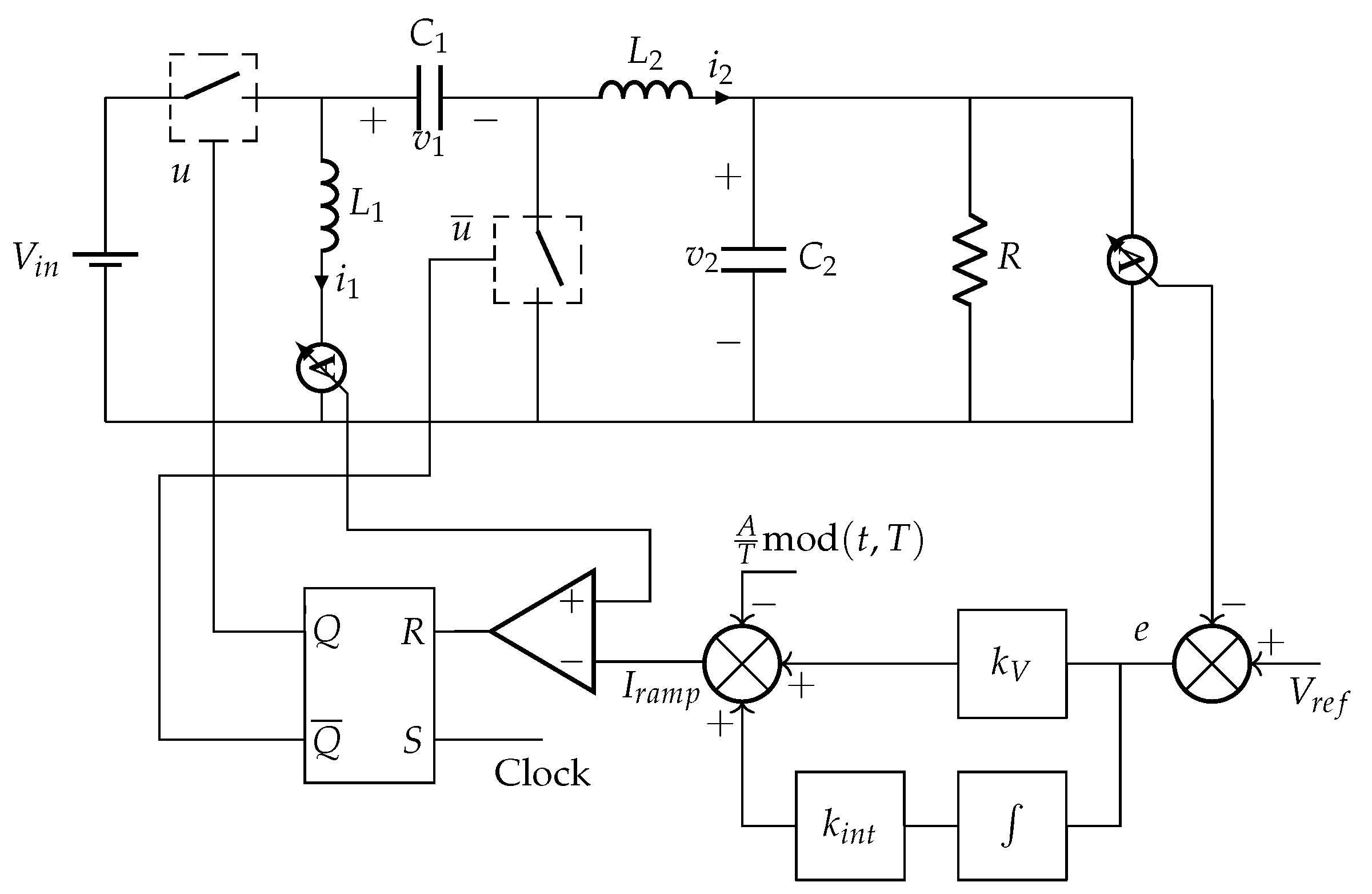
2. Synchronous ZETA Converter

2.1. Mathematical Model

The sZETA converter is schematized in Figure 1. In its simplest form, it is composed by an input voltage source $V_{in}$ and five linear elements, namely two capacitors with capacitance $C_1$ and $C_2$, two coils characterized by the inductance $L_1$ and $L_2$, and the load resistance R. Additionally, two synchronous switches complete the design: whenever the control signal $u=1$, the main switch is set to the ON position and the complementary switch is automatically set to the OFF position ($\overline{u}=0$), and vice versa. The state of the sZETA converter is completely described by the currents flowing through the coils ($i_1$ and $i_2$) and the voltages across the capacitors $v_1$ and $v_2$. Notice that, since we are interested in a theoretical approach to the stability of the converter, all elements are assumed to be ideal. The output voltage of the converter is given by $v_2$. Furthermore, with the aim of defining a PI control in Section 2.2, we extend the state vector to include the integral of the error between a desired output $V_{ref}$ and the output voltage, namely $e=V_{ref}-v_2$. Altogether, we can fully describe the sZETA converter via the state vector:

$$\mathbf{x}=\left[\begin{array}{c}{x}_1\\ x_2\\ x_3\\ x_4\\ x_5\end{array}\right]:=\left[\begin{array}{c}{i}_1\\ i_2\\ v_1\\ v_2\\ \int edt\end{array}\right]$$

(1)

which evolves according to the following equations:

$$\dot{\mathbf{x}}=\left\{\begin{array}{cc}{\mathbf{f}}_{ON}\left(\mathbf{x}\right)\hfill & \mathrm{if}u=1\hfill \\ {\mathbf{f}}_{OFF}\left(\mathbf{x}\right)\hfill & \mathrm{if}u=0\hfill \end{array}\right.$$

(2)

where

$${\mathbf{f}}_{ON}=\left[\begin{array}{c}{V}_{in}/L_1\\ v_1/L_2-v_2/L_2+V_{in}/L_2\\ -i_2/C_1\\ i_2/C_2-v_2/\left(R{C}_2\right)\\ V_{ref}-v_2\end{array}\right]{\mathbf{f}}_{OFF}=\left[\begin{array}{c}-v_1/L_1\\ -v_2/L_2\\ i_1/C_1\\ i_2/C_2-v_2/\left(R{C}_2\right)\\ V_{ref}-v_2\end{array}\right]$$

(3)

are the vector fields that govern the dynamics in each one of the topologies defined by the position of the main switch. The gain of the sZETA converter depends on the value of the duty cycle d, i.e., the fraction of time during a PWM cycle that the switch remains in the ON position. It can be shown that the gain of the controller is given by [18]

$$\mathcal{G}=\frac{d}{1-d}$$

(4)

which means that the sZETA can work as a step-down ($d<0.5$) or step-up converter ($d>0.5$).

2.2. Control via Ramp Compensation

Now, we add a feedback loop to the system which allows us to obtain the desired output value $V_{ref}$. To do so, we implement a ramp compensation which is schematized in the feedback loop of Figure 1. The ramp compensation $I_{ramp}$ is formed by a ramp periodic signal of period T that is subtracted at the output of a PI controller. The PI control operates over the output voltage and its aim is to reject disturbances while eliminating the steady state error and controlling the transient state. Notice that the PI controller corresponds to an external control loop of the voltage, as:

$$\begin{array}{c}\hfill I_{ramp}=k_V(V_{ref}-v_2)+k_{int}{x}_5-\frac{A}{T}mod(t,T),\end{array}$$

(5)

where $k_V$ and $k_{int}$ are the gains of the PI control and A is the ramp slope. At the beginning of the cycle, the main switch is set to the ON position ($u=1$). The main switch is then set to the OFF position ($u=0$) when $I_{ramp}$ is equal to the current in the first coil $i_1$ (internal loop), or equivalently when:

$$\begin{array}{c}\hfill i_1=I_{ramp}.\end{array}$$

(6)

After this, the switch remains OFF until the beginning of the next cycle, completing the design of the controller. The switching condition (6) can be rewritten in the form $h_r(\mathbf{x},t)=0$ with

$$\begin{array}{c}\hfill h_r(\mathbf{x},t)=k_V(V_{ref}-v_2)+k_{int}{x}_5-\frac{A}{T}mod(t,T)-i_1.\end{array}$$

(7)

Figure 2 shows an example of the ramp controlled sZETA converter. In Figure 2A, we display the evolution of $I_{ramp}$ and $i_1$, during two cycles in the steady state. It is possible to see that, when both functions are equal, the control signal changes from $u=1$ to $u=0$ (Figure 2B). Figure 2C shows the evolution of the voltages $v_1$ and $v_2$ and depicts how, after a short transient, the output voltage (red line) asymptotically converges to the reference value $V_{ref}$ (dashed black line). Throughout the paper, we make use of the values of the parameters shown in

Table 1. Parameter values used throughout the paper.

Parameter Values
$V_{in}$ = 10 V	$V_{ref}=15$ V
$C_1=100 \mathsf{\mu }$F	$C_1=220 \mathsf{\mu }$F
$L_1=100 \mathsf{\mu }$H	$L_2=55 \mathsf{\mu }$H
$R=100$$\mathsf{\Omega }$	$T=50 \mathsf{\mu }$s
$k_V$ = 1	$k_{int}$ = 500

unless otherwise stated.

A few words must be said about the values of the gains chosen. On the one hand, $k_V$ was chosen to be relatively small to avoid oscillatory behavior during transient state. Moreover, $k_{int}$ has a rather large value to guarantee fast convergence to the steady state and small steady error. Finally, the most critical parameter is the ramp compensation, i.e., the slope A, which is tuned in such a way to guarantee stable operation in a set of points chosen in the range of parameters that we use in this paper. To do so, we make use of the stability criteria that we describe in the following section.

3. Stability Analysis

3.1. Floquet Multipliers

As shown in Figure 2, the ideal operation of the sZETA converter consists of a periodic orbit with period T, which commutes the position of the switch between 1 and 0 and assures that the orbit oscillates around the desired operation point. We now turn our attention to describe the stability of this periodic orbit, by making use of Floquet theory.

Let us assume a periodic solution ${\mathbf{x}}_p\left(t\right)={\mathbf{x}}_p(t+T)$. According to Floquet theory, the stability of an infinitesimally perturbation around the reference orbit $\delta {\mathbf{x}}_p$ evolves from one period to the other as:

$$\delta {\mathbf{x}}_p(t+T)=M\delta {\mathbf{x}}_p\left(t\right).$$

(8)

Here, M is the monodromy matrix and is equal to the state transition matrix $\mathsf{\Phi }(\mathbf{x}\left(t_0\right),t_0,t)$ evaluated at $t=t_0+T$, namely:

$$\begin{array}{c}\hfill M=\mathsf{\Phi }(\mathbf{x}\left(t_0\right),t_0,t_0+T)\end{array}$$

(9)

The eigenvalues of the monodromy matrix ${\mu }_i$ are the so-called Floquet multipliers and indicate the stability of the periodic orbit as follows:

• If $|{\mu }_i|<1$ for all i, then the orbit is stable.
• If at least one $|{\mu }_i|>1$, the orbit is unstable.

The definition of the monodromy matrix in Equation (9) is valid for smooth systems. However, consider that the sZETA converter switches its dynamics from topology $u=1$ to topology $u=0$ whenever condition (7) is met, which requires special treatment for the calculation of the monodromy matrix. Let us call ${\mathbf{x}}^{*}$ the state of the system where $h_r({\mathbf{x}}^{*},t^{*})=0$, and the corresponding switching time is $t^{*}$. It is easy to see that $t^{*}$ can be expressed as $t^{*}=t_0+dT$ if we set $t_0$ at the beginning of the ramp cycle. Without loss of generality, we can make $t_0=0$, therefore ${\mathbf{x}}^{*}=\mathbf{x}\left(dT\right)$. Then, for a non-smooth system that switches its dynamics from a vector field ${\mathbf{f}}_{ON}$ to ${\mathbf{f}}_{OFF}$, the monodromy matrix can be constructed as follows (see [31] for a detailed explanation):

$$\begin{array}{c}\hfill M={\mathsf{\Phi }}_{OFF}(\mathbf{x}\left(dT\right),dT,T)·\mathcal{S}·{\mathsf{\Phi }}_{ON}(\mathbf{x}\left(0\right),0,dT),\end{array}$$

(10)

where ${\mathsf{\Phi }}_{ON}$ (${\mathsf{\Phi }}_{OFF}$) are the state transition matrices associated with ${\mathbf{f}}_{ON}$ (${\mathbf{f}}_{OFF}$). Thanks to the linear nature of each individual vector field, the state transition matrices can be straightforwardly calculated as:

$$\begin{array}{ccc}\hfill {\mathsf{\Phi }}_{ON}& =& e^{A_{ON}Td}\hfill \end{array}$$

(11)

$$\begin{array}{ccc}\hfill {\mathsf{\Phi }}_{OFF}& =& e^{A_{OFF}T(1-d)}\hfill \end{array}$$

(12)

with

$$\begin{array}{ccc}\hfill A_{ON}& =& \frac{\partial {\mathbf{f}}_{ON}}{\partial \mathbf{x}}=\left[\begin{array}{ccccc}0& 0& 0& 0& 0\\ 0& 0& 1/L_2& -1/L_2& 0\\ 0& -1/C_1& 0& 0& 0\\ 0& 1/C_2& 0& -1/\left(R{C}_2\right)& 0\\ 0& 0& 0& -1& 0\end{array}\right]\hfill \end{array}$$

(13)

$$\begin{array}{ccc}\hfill A_{OFF}& =& \frac{\partial {\mathbf{f}}_{OFF}}{\partial \mathbf{x}}=\left[\begin{array}{ccccc}0& 0& -1/L_1& 0& 0\\ 0& 0& 0& -1/L_2& 0\\ 1/C_1& 0& 0& 0& 0\\ 0& 1/C_2& 0& -1/\left(R{C}_2\right)& 0\\ 0& 0& 0& -1& 0\end{array}\right]\hfill \end{array}$$

(14)

The matrix $\mathcal{S}$ is the so-called saltation matrix, which accounts for the non-smoothness at the switching time $t^{*}$ and has the form:

$$\mathcal{S}=I+\frac{({\mathbf{f}}_{OFF}\left({\mathbf{x}}^{*}\right)-{\mathbf{f}}_{ON}\left({\mathbf{x}}^{*}\right))·{\mathbf{n}}^T}{{\mathbf{n}}^T·{\mathbf{f}}_{ON}\left({\mathbf{x}}^{*}\right)+\frac{\partial h_r(\mathbf{x},t)}{\partial t}},$$

(15)

where $\mathbf{n}=\nabla h_r(\mathbf{x},t)$ is the normal vector to the switching surface, which in our case can be written as

$$\mathbf{n}={[-1,0,0,k_V,k_{int}]}^T,$$

(16)

and, similarly,

$$\frac{\partial h_r(\mathbf{x},t)}{\partial t}=-\frac{A}{T}.$$

(17)

With this, we can summarize the steps to establish the stability of a Period 1 orbit in the following algorithm:

• Find the state at the beginning of the periodic orbit $\mathbf{x}\left(0\right)$ and the duty cycle d that fulfill the following conditions

  $$\begin{array}{ccc}\hfill \mathbf{x}\left(0\right)& =& \mathbf{x}\left(T\right)\hfill \\ \hfill h\left(\mathbf{x}\right(dT),dT)& =& 0\hfill \end{array}$$

  (18)
• With the solution d and $\mathbf{x}\left(0\right)$, calculate the state transition matrices (11) and (12) and the saltation matrix (15), to obtain the monodromy matrix (10).
• Obtain the Floquet multipliers as the eigenvalues of M.

3.2. Lyapunov Exponents

Lyapunov exponents provide an additional analysis tool to study the orbits in power converters [40]. Recall that Floquet multipliers are restricted to the study of periodic orbits. However, it can be the case that a power converter shows more complex phenomena that go beyond a Period 1 solution, such as quasi-periodicity and chaos. To quantify this, one has to make use of Lyapunov exponents. For a system whose evolution is governed by $\dot{\mathbf{x}}=\mathbf{f}\left(\mathbf{x}\right)$, given an infinitesimally small perturbation $\delta \mathbf{x}\left(0\right)$ around a reference orbit (notice that here we do not restrict the perturbation to a given periodic solution as in Section 3.1), the maximal Lyapunov exponent ${\lambda }_{max}$ is defined as:

$${\lambda }_{max}=\underset{t\to \infty }{lim}\frac{1}{t}log\frac{\left|\right|\delta \mathbf{x}\left(t\right)\left|\right|}{\left|\right|\delta \mathbf{x}\left(0\right)\left|\right|}.$$

(19)

The maximal Lyapunov exponent quantifies the rate of convergence (${\lambda }_{max}<0$) or divergence (${\lambda }_{max}>0$) of the reference orbit and the infinitesimally perturbed one. Hence, ${\lambda }_{max}$ describes the nature of a given orbit as follows:

• If ${\lambda }_{max}<0$, the attractor is a stable fixed point.
• If ${\lambda }_{max}=0$, the attractor is a stable periodic (or quasi-periodic) orbit.
• If ${\lambda }_{max}>0$, the attractor is chaotic.

In Equation (19), $\delta \mathbf{x}\left(t\right)$ is the evolution in time of the infinitesimal perturbation (also called tangent space) and its dynamics is governed by the variational equation

$$\delta \dot{\mathbf{x}}=\frac{\partial \mathbf{f}\left(\mathbf{x}\right)}{\partial \mathbf{x}}\delta \mathbf{x}$$

(20)

As in Section 3.1, the tangent evolution needs to be specially treated at the times where the system changes from a vector field to another. To solve this, we make use of the Mueller algorithm to solve the tangent evolution for systems with discontinuities [50]. We first describe the general procedure.

Let ${\mathbf{x}}^{-}$ be the state vector right before a discontinuous event, which occurs when an indicator function $h\left(\mathbf{x}\right)=0$. In addition, let ${\mathbf{x}}^{+}$ be the state right after the discontinuous event which may undergo a discontinuous change given by a so-called impact function $\mathbf{g}\left({\mathbf{x}}^{-}\right)$ that maps the state of the system right before/right after the discontinuous event, namely ${\mathbf{x}}^{+}=\mathbf{g}\left({\mathbf{x}}^{-}\right)$. Similarly, ${\mathbf{f}}^{-}$ and ${\mathbf{f}}^{+}$ are the vector fields that govern the dynamics before and after the discontinuity, respectively. With these considerations, the correction of the tangent space at the discontinuity is:

$$\delta {\mathbf{x}}^{+}=G\left({\mathbf{x}}^{-}\right)\delta {\mathbf{x}}^{-}+[G\left({\mathbf{x}}^{-}\right){\mathbf{f}}^{-}\left({\mathbf{x}}^{-}\right)-{\mathbf{f}}^{+}\left({\mathbf{x}}^{+}\right)]\delta t.$$

(21)

In Equation (21), $\delta t$ is defined as:

$$\delta t=\frac{-\mathbf{H}\left({\mathbf{x}}^{-}\right)\delta {\mathbf{x}}^{-}}{\mathbf{H}\left({\mathbf{x}}^{-}\right){\mathbf{f}}^{-}\left({\mathbf{x}}^{-}\right)}.$$

(22)

and

$$G\left(\mathbf{x}\right)=\frac{\partial \mathbf{g}\left(\mathbf{x}\right)}{\partial \mathbf{x}};\mathbf{H}\left(\mathbf{x}\right)=\frac{\partial h\left(\mathbf{x}\right)}{\partial \mathbf{x}}.$$

(23)

In order to apply the Mueller algorithm to the sZETA converter controlled via ramp compensation, it is convenient to express the dynamics of the system in an autonomous way including the evolution of the ramp. To do this, we extend the original system (3) to account for the ramp dynamics, making $\tilde{\mathbf{x}}:={[i_1,i_2,v_1,v_2,\int edt,x_6]}^T$ where $x_6=-\frac{A}{T}t$, hence:

$${\tilde{\mathbf{f}}}_{ON}=\left[\begin{array}{c}{V}_{in}/L_1\\ v_1/L_2-v_2/L_2+V_{in}/L_2\\ -i_2/C_1\\ i_2/C_2-v_2/\left(R{C}_2\right)\\ V_{ref}-v_2\\ -A/T\end{array}\right]{\tilde{\mathbf{f}}}_{OFF}=\left[\begin{array}{c}-v_1/L_1\\ -v_2/L_2\\ i_1/C_1\\ i_2/C_2-v_2/\left(R{C}_2\right)\\ V_{ref}-v_2\\ -A/T\end{array}\right]$$

(24)

In this framework, two discontinuous events occur and therefore two different corrections to the tangent evolution must be done:

• The first one corresponds to the transition of the switch from ON to OFF position, which is given by the indicator function

  $${\tilde{h}}_r\left(\tilde{\mathbf{x}}\right)=k_V(V_{ref}-v_2)+k_{int}{x}_5+x_6-i_1$$

  (25)
  Here, the fields ${\mathbf{f}}^{-}={\tilde{\mathbf{f}}}_{ON}$, ${\mathbf{f}}^{+}={\tilde{\mathbf{f}}}_{OFF}$, and the states do not change their values abruptly, hence the impact function ${\tilde{\mathbf{g}}}_r\left(\tilde{\mathbf{x}}\right)$ is trivially

  $${\tilde{\mathbf{g}}}_r\left(\tilde{\mathbf{x}}\right)=[i_1,i_2,v_1,v_2,x_5,x_6].$$

  (26)
  With these ingredients, the different terms to be applied in Equations (21) and (22) are:

  $${\mathbf{H}}_r=[-k_I,0,0,-k_V,k_{int},1]$$

  (27)

  and

  $$G_r=I$$

  (28)
• The second discontinuous event occurs when the ramp resets to 0 at the end of every cycle, or equivalently when $x_6=-A$ which corresponds to the indicator function

  $${\tilde{h}}_c\left(\tilde{\mathbf{x}}\right)=x_6+A$$

  (29)
  Special care must be taken at this point. If the duty cycle is not saturated, then at each T-cycle ${\mathbf{f}}^{-}={\tilde{\mathbf{f}}}_{OFF}$ and ${\mathbf{f}}^{+}={\tilde{\mathbf{f}}}_{ON}$. However, it might happen that the cycle is saturated and the switch remained in the ON position during the whole period, in which case ${\mathbf{f}}^{-}={\mathbf{f}}^{+}={\tilde{\mathbf{f}}}_{ON}$. In both cases, $x_6$ changes its value abruptly to a constant value $x_6=0$, hence the impact function is:

  $${\tilde{\mathbf{g}}}_c\left(\tilde{\mathbf{x}}\right)=[i_1,i_2,v_1,v_2,x_5,0],$$

  (30)

  which leads to

  $${\mathbf{H}}_c=[0,0,0,0,0,1]$$

  (31)

  and

  $$G_c=\left[\begin{array}{cccccc}1& 0& 0& 0& 0& 0\\ 0& 1& 0& 0& 0& 0\\ 0& 0& 1& 0& 0& 0\\ 0& 0& 0& 1& 0& 0\\ 0& 0& 0& 0& 1& 0\\ 0& 0& 0& 0& 0& 0\end{array}\right]$$

  (32)

With these corrections, the ${\lambda }_{max}$ calculation can be summarized in the following steps:

• Evolve the extended system:

  $$\left[\begin{array}{c}\dot{\tilde{\mathbf{x}}}\\ \delta \dot{\tilde{\mathbf{x}}}\end{array}\right]=\left\{\begin{array}{ccc}\left[\begin{array}{c}\begin{array}{c}{\tilde{\mathbf{f}}}_{ON}\left(\tilde{\mathbf{x}}\right)\hfill \\ \frac{\partial {\tilde{\mathbf{f}}}_{ON}\left(\tilde{\mathbf{x}}\right)}{\partial \tilde{\mathbf{x}}}\delta \tilde{\mathbf{x}}\hfill \end{array}\end{array}\right]\hfill & \mathrm{if}\hfill & u=1\hfill \\ \\ \left[\begin{array}{c}\begin{array}{c}{\tilde{\mathbf{f}}}_{OFF}\left(\tilde{\mathbf{x}}\right)\hfill \\ \frac{\partial {\tilde{\mathbf{f}}}_{OFF}\left(\tilde{\mathbf{x}}\right)}{\partial \tilde{\mathbf{x}}}\delta \tilde{\mathbf{x}}\hfill \end{array}\end{array}\right]\hfill & \mathrm{if}\hfill & u=0\hfill \end{array}\right.$$

  (33)

  in the interval $[t_0,t_0+\tau ]$ with randomly chosen initial conditions for $\delta \tilde{\mathbf{x}}\left(t_0\right)$, such that $\left|\right|\delta \tilde{\mathbf{x}}\left(t_0\right)\left|\right|=1$.
• During the evolution, identify the times of each of the possible discontinuous events given by (25) or (29) and apply the correction (21) in accordance with the nature of the discontinuous event.
• When $t=t_0+\tau$, calculate and store

  $${\lambda }_i=\frac{1}{\tau }log\frac{\left|\right|\delta \tilde{\mathbf{x}}\left(t\right)\left|\right|}{\left|\right|\delta \tilde{\mathbf{x}}\left(t_0\right)\left|\right|}$$
• Set $t_0=t_0+\tau$ and renormalize $\left|\right|\delta \tilde{\mathbf{x}}\left(t_0\right)\left|\right|=1$.
• Repeat Steps 1–4 for a sufficiently large number of steps N.
• Calculate the maximal Lyapunov exponent as:

  $${\lambda }_{max}=\frac{1}{N}\sum _{i=1}^N{\lambda }_i,$$

4. Results

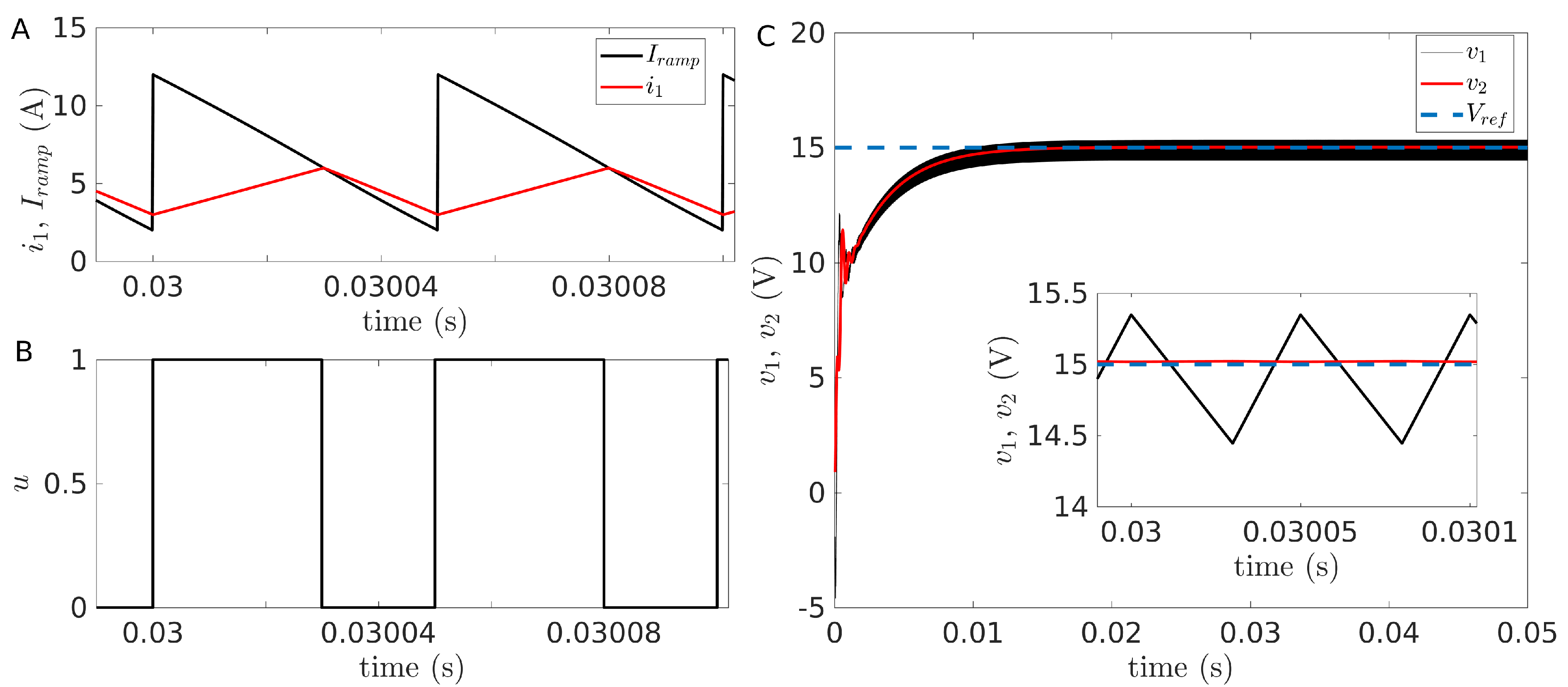
4.1. Ramp Compensation Design

We first sought to choose a suitable value of the ramp compensation slope A, as it is one of the most critical parameters in the control design. To do so, we calculated the stability of the Period 1 orbit via Floquet multipliers in the biparametric space $(A,V_{in})$ with $R=100 \mathsf{\Omega }$. This situation is depicted in Figure 3 for different values of $V_{ref}$. An interesting observation is that, for small values of $V_{ref}$, the system tends to lose stability when two conditions are met: (i) $V_{in}\approx V_{ref}$; and (ii) A is rather large, as seen in the dark red area in Figure 3A, which corresponds to $|{\mu }_{max}|>1$. Interestingly, at increasing values of $V_{ref}$, the controller does not lose stability anymore at large A, and the conditions for stability loss are: (i) $V_{in}<V_{ref}$ (equivalently when the sZETA converter works as a boost); and (ii) A is small, which produces the red triangular areas in Figure 3B–D. Since one of the main attributes of the sZETA converter is the ability to work both as a step-down and step-up converter, we chose a value of A which guarantees stability for most of the cases depicted in Figure 3. This value corresponds to $A=10$, which is shown with the magenta line in all panels. In the next section, a deep stability analysis considering continuous variation of not only $V_{in}$ and $V_{ref}$ but also R is presented.

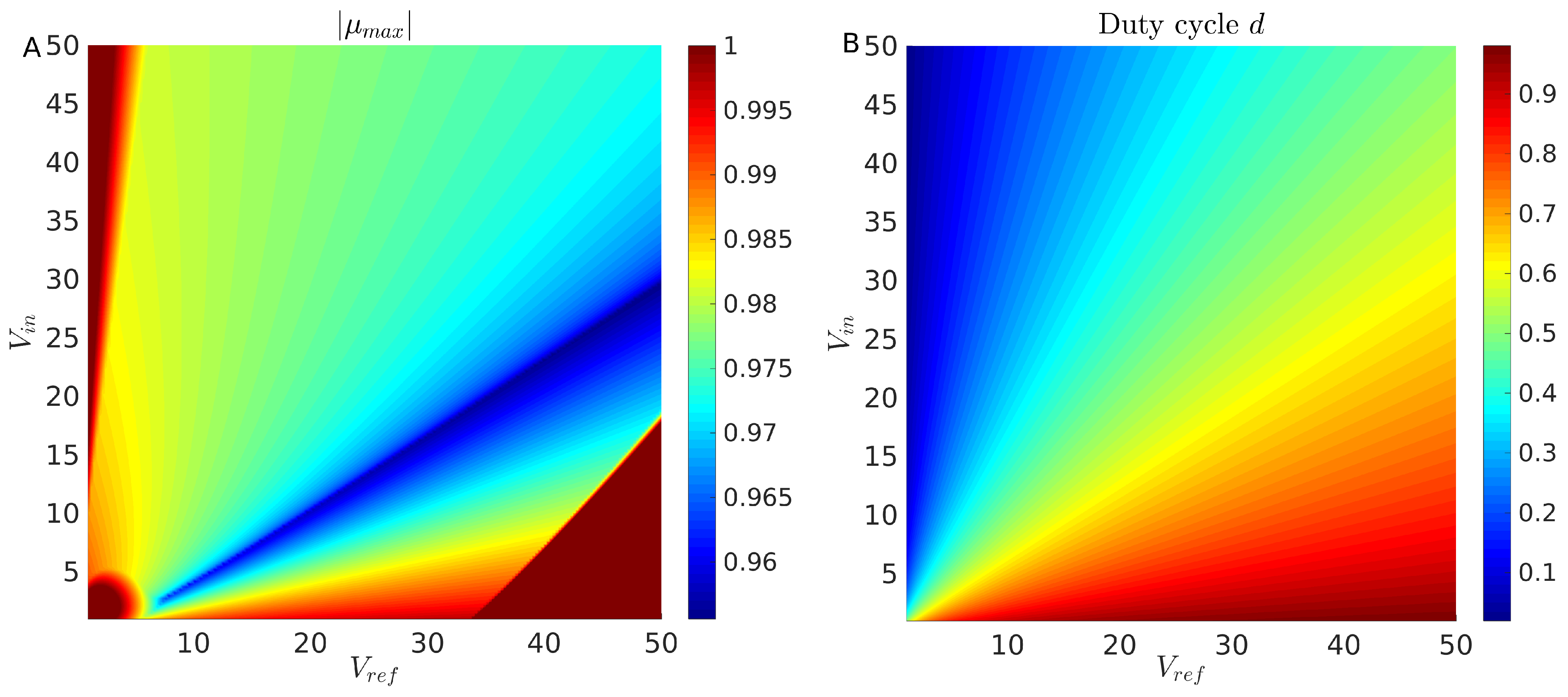
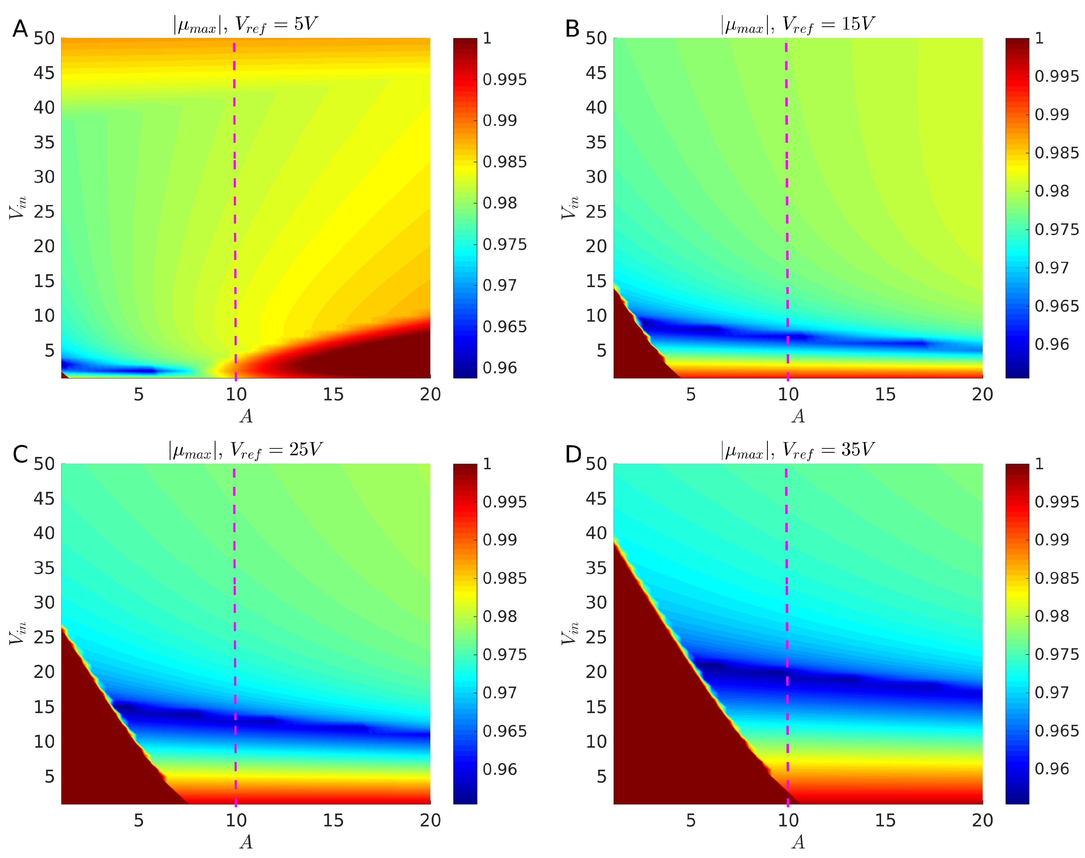
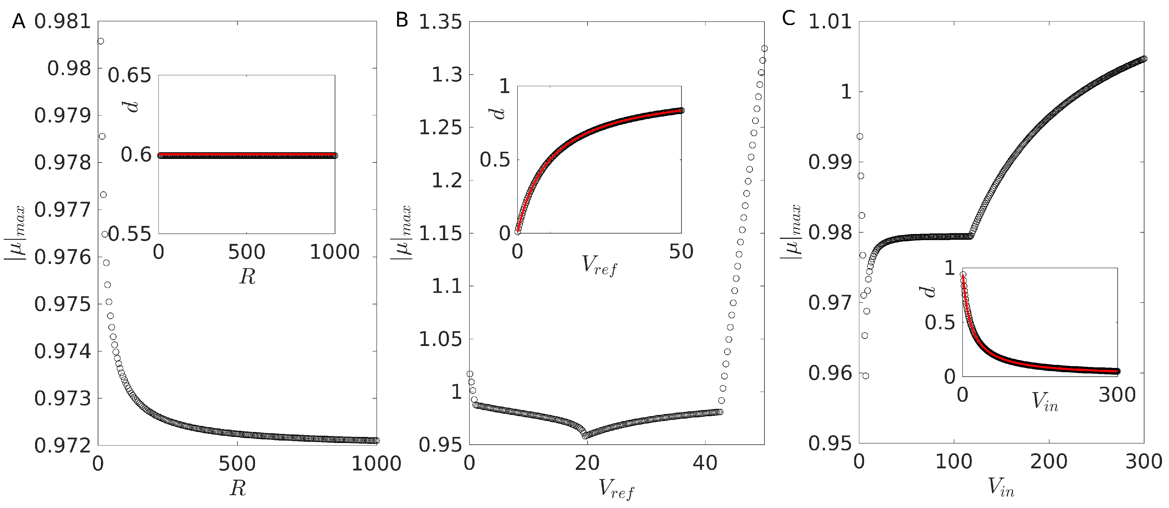
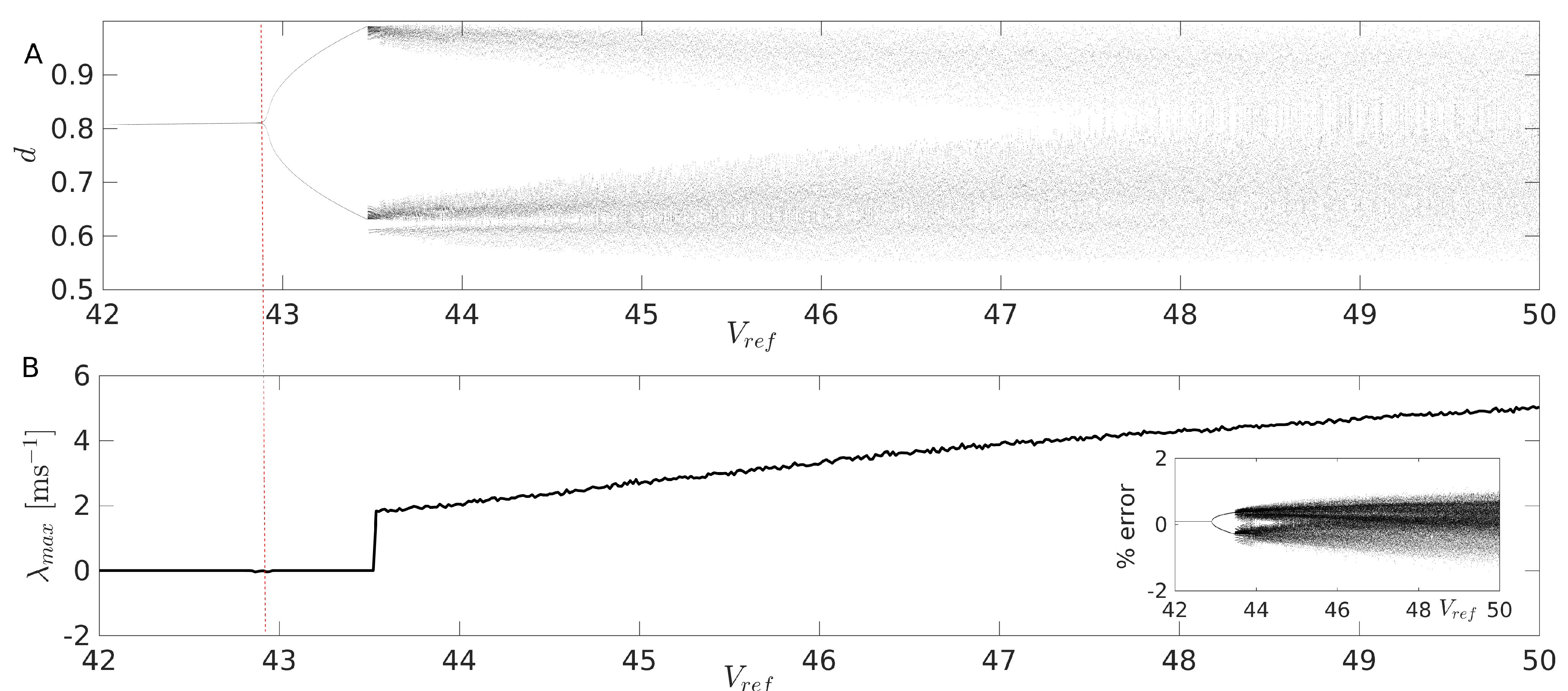
4.2. Stability Regions

Now that we have chosen a suitable value of A, we aim to characterize the stability regions in the ramp compensation controlled sZETA converter at variations of different parameters and to characterize the mechanisms by which the stability is lost. To do this, we calculate the stability of the Period 1 solution taking R, $V_{in}$, and $V_{ref}$ as bifurcation parameters (recall that the nominal parameters are $R=100$$\mathsf{\Omega }$, $V_{ref}=15$ V, and $V_{in}=10$ V). The results are depicted in Figure 4. It is possible to see in Figure 4A that the load has little effect on the stability of the controller, as testified by ${\left|\mu \right|}_{max}<1$ in the whole range of resistances $R\in [1 \mathsf{\Omega },1000 \mathsf{\Omega }]$ that we considered. It is also not surprising that the value of the duty cycle remains unchanged over the whole range and very close to the expected gain $\mathcal{G}$ defined in Equation (4), as the gain only depends on the values $V_{in}$ and $V_{ref}$. Next, we focus on the evolution of ${\left|\mu \right|}_{max}$ as a function of $V_{ref}$ in Figure 4B. Here, we can observe that the orbit is stable in an ample range of $V_{ref}$, and it only loses stability at either very small references ($V_{ref}<1$ V) or very large ones ($V_{ref}>42.9$ V). This of course corresponds to very low or very high values of the duty cycle where power converters do not perform adequately. As above, the duty cycle solution obtained by solving (4) is in good agreement with the expected gain. Finally, we found a similar behavior choosing $V_{in}$ as the bifurcation parameter (see Figure 4C). Namely, the system loses stability only at very large values of $V_{in}$ corresponding to extreme values of the duty cycle. This suggests that the peak-current with ramp compensation is a quite stable strategy, except for cases in which the gain is either very small of very large.

To test this hypothesis, we proceeded to calculate ${\left|\mu \right|}_{max}$ in the two-dimensional parameter space $(V_{ref},V_{in})$ and the value of the duty cycle consistent with the Period 1 solution in Equation (18). The results are shown in Figure 5, where it can be seen that, indeed, the regions where the Period 1 orbit loses stability are those when the ratio $V_{in}$/$V_{ref}$ is either too large or too small (bright red regions in Figure 5A). These are indeed parameter regions where the duty cycle has very large or very low values (see Figure 5B), hence supporting the initial hypothesis. A rather interesting exception appears for cases in which $V_{in}\approx V_{ref}<5$ V. This is not surprising, because, as shown in Figure 3A, for the chosen value of the ramp slope A, there is a region of small and comparable values of $V_{ref}$ and $V_{in}$ where the controller is unstable. This result indicates that the proposed controller handles much better medium to high values of voltages, at least for the parameters chosen here.

To better understand the mechanism of stability loss, we proceeded to calculate the bifurcation diagram of the duty cycle in the interval $V_{ref}\in$ [42 V, 50 V] at fixed $V_{in}=10$ V. As depicted in Figure 4B, we expect a stability change at $V_{ref}\approx 42.9$ V. The bifurcation diagram of the duty cycle shows the transition to a Period 2 orbit at that same value, as shown with the red vertical line in Figure 6A. Such orbit remains stable, as testified by ${\lambda }_{max}=0$ (see Figure 6B), up to the value $V_{ref}\approx 43.54$ V, where the duty cycle starts saturating and producing seemingly chaotic values of d. The chaotic nature of the solutions after this critical value of $V_{ref}$ is indeed revealed by ${\lambda }_{max}>0$ after this point. From the definition of ${\lambda }_{max}$, it is possible to deduce that two nearby trajectories will be completely uncorrelated after a few milliseconds. The transition to chaos due to saturated d has been described previously as the route to chaos via skipped cycles in the literature [51]. Despite the fact that the chaotic regime is definitely undesired in any real application, it should be noticed that, nonetheless, the values of the error remain rather small (<2%) in the whole studied interval (see inset).

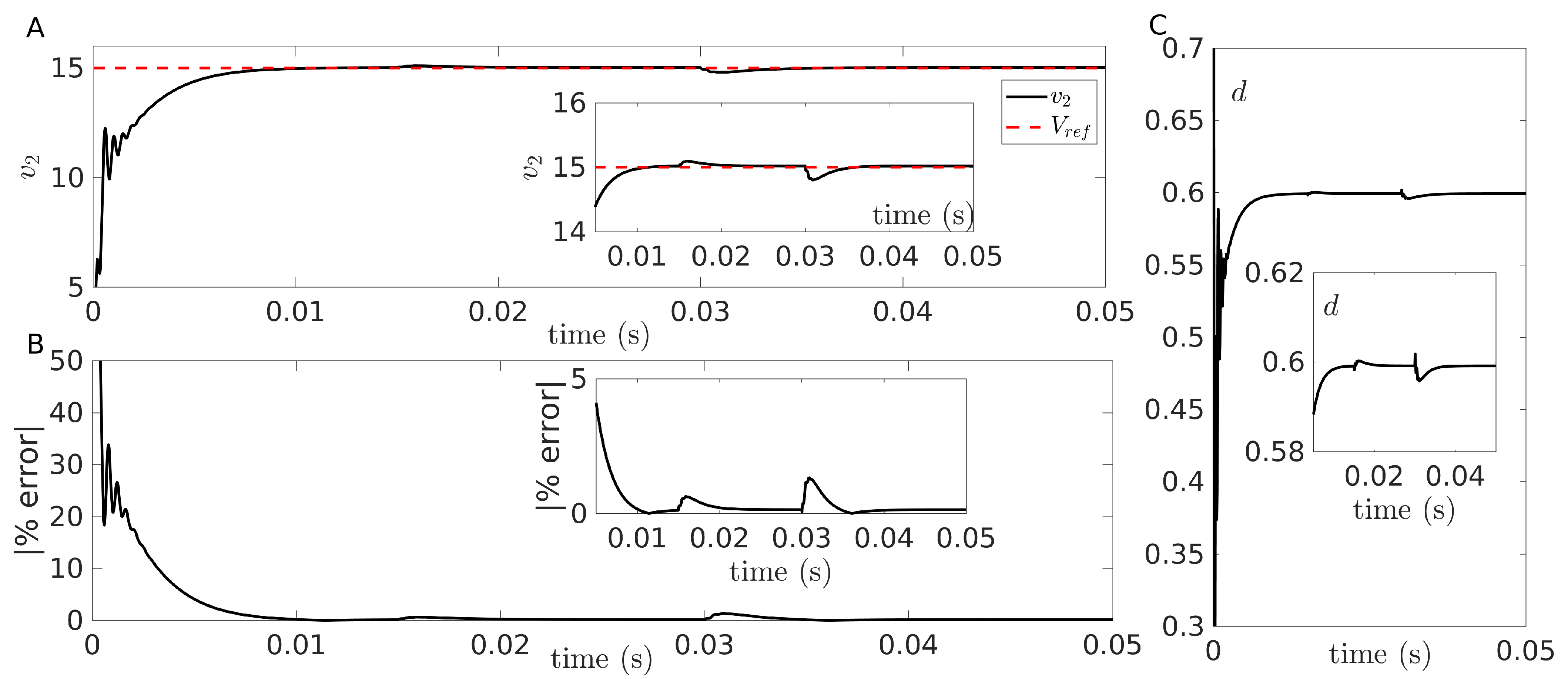
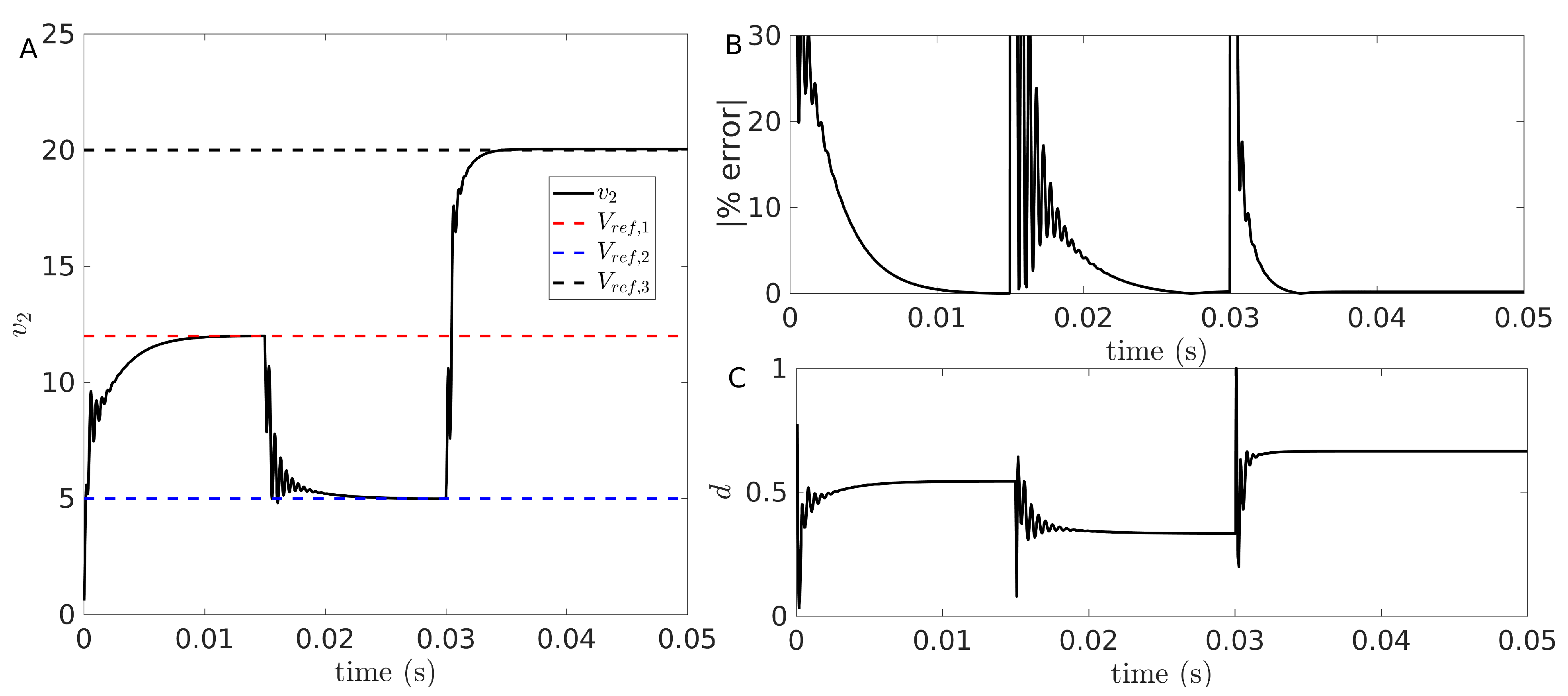
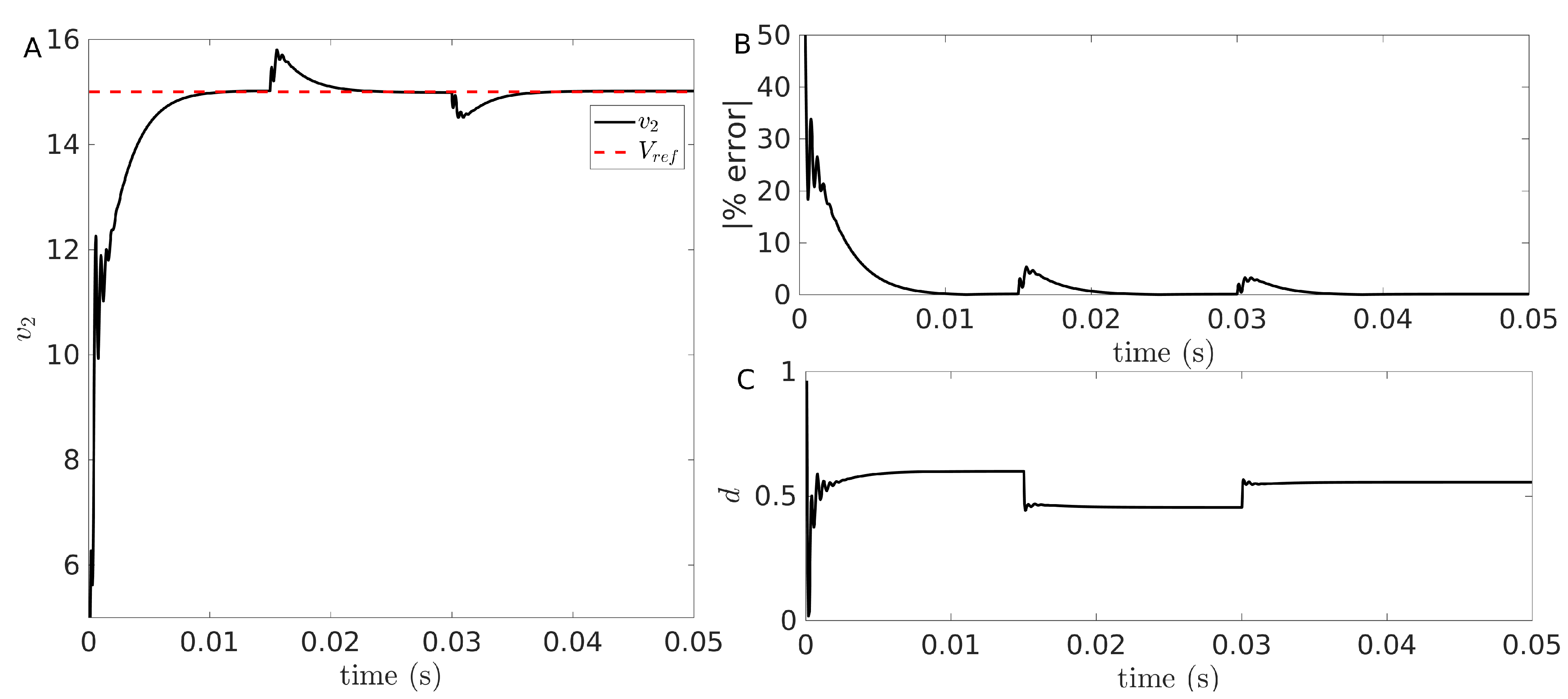
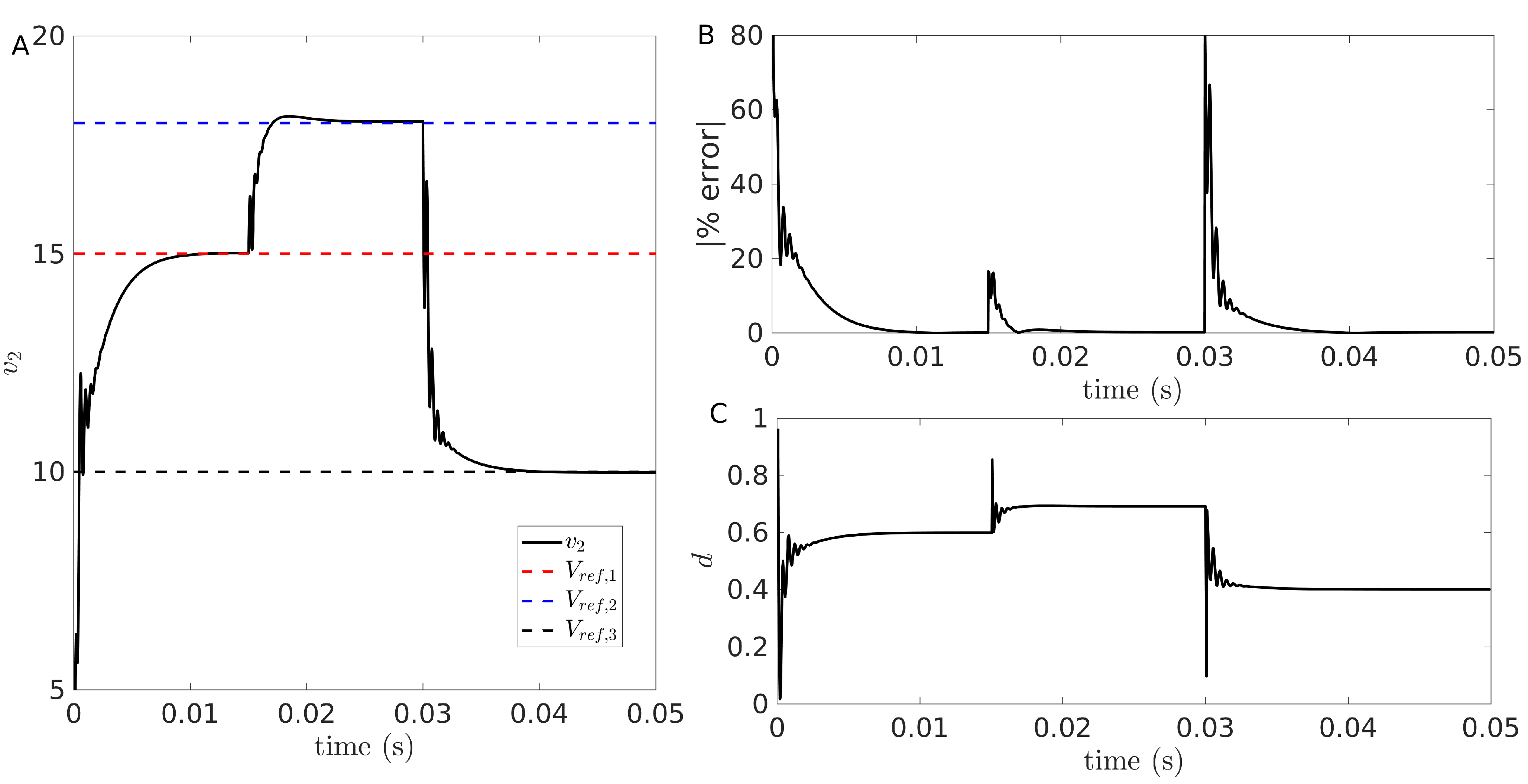
4.3. Disturbance Rejection

We now proceed to evaluate the performance of the ramp controlled sZETA converter under different types of perturbations. First, we focus on disturbances at the load R. This simulation is depicted in Figure 7. In this figure, R is set to the nominal value of $100 \mathsf{\Omega }$, where one can see that the converter rapidly converges to the reference voltage in around 8 ms, starting from $\mathbf{x}\left(0\right)=\mathbf{0}$ (see Figure 7A), while the error rapidly decreases below 1% (Figure 7B). At $t=15$ ms, the load is abruptly changed to $R=200 \mathsf{\Omega }$, where it again rapidly responds to the perturbation by transiently changing the duty cycle, until it relaxes again to the expected value $d=(V_{ref}/V_{in})/(1+V_{ref}/V_{in})$, which for the chosen values of the reference and input voltage corresponds to $d=0.6$ (see Figure 7C). Finally, another perturbation is presented to the system at $t=30$ ms, where R is again changed to $50 \mathsf{\Omega }$. It can be seen here that the controller handles the perturbation in a satisfactory manner. In fact, the last two disturbances are practically negligible. This means that, once the system reaches the steady state, disturbances in the load are unimportant for the system’s performance.

Similarly, we performed a perturbation analysis in a more interesting set-up, i.e., by introducing disturbances in $V_{ref}$ in such a way that the converter switches its behavior from step-up to step-down regime. This situation is depicted in Figure 8. From the time trace of the output voltage, we can see that the system reaches the three desired values of the reference despite the rather large deviations from one value to the other. Notice that, in the second transition, $V_{ref}$ changes from $V_{ref,2}=5$ V to $V_{ref,3}=20$ V, which corresponds to a percent change of $300\%$. Even in this extreme case, the system reaches steady operation in approximately 5 ms, as seen by the small error values in Figure 8B a few milliseconds after the presentation of the disturbance. As expected, the transitions to different reference voltages are accompanied by variations in the steady state value of the duty cycle, which meet the expected value of the gain $\mathcal{G}$ (Figure 8C).

We performed the same perturbation analysis with $V_{in}$ as a perturbation parameter. Following the same procedure as for $V_{ref}$, $V_{in}$ was varied in such a way that the sZETA converter alternates between step-up and step-down behavior. In particular, it transits from step-up to step-down at $t=15$ ms and returns to a step-up regime at $t=30$ ms, as shown in Figure 9. As reported with the disturbances in $V_{ref}$, the converter rapidly reaches steady evolution in all the considered cases, despite the rather large variations of $V_{in}$. It is worth noticing that variations in $V_{in}$ produce transient oscillations of smaller amplitude when compared with variations of $V_{ref}$, which produces lower deviations of the error (see Figure 9B) that is kept below $10\%$. This is also reflected in a much faster evolution of the duty cycle towards the asymptotic value, as seen in Figure 9C. This phenomenon can be explained because changing the input voltage requires only the adjustment of the currents flowing trough the coils, while the capacitors’ voltages are kept very close to the already desired value. On the contrary, when $V_{ref}$ changes, it is necessary for all the states, including the voltages of the capacitors, to adjust their values.

Finally, with the aim of further showing the robustness of the controller, we carried out a mixed perturbation test in which all three parameters were varied simultaneously. This scenario is shown in Figure 10, and the results support the initial findings, namely that the controller is robust to even large variations from the nominal values of the parameters, including transitions from step-up (for $t<30$ ms) to step-down regimes ($t>30$ ms). In this figure, it is possible to notice an additional feature of this converter that is not clearly observable in Figure 7, namely that the last transition, which corresponds to the largest value of R, has a much faster transient response. Indeed, the transient time elapsed for the reference voltage $V_{ref,2}=18$ V to $V_{ref,3}=10$ V is significantly smaller than the initial transient taken to reach $V_{ref,1}=10$ V (≈5 ms vs. ≈10 ms, respectively). This is despite the fact that the initial errors are comparable (see Figure 10B,C). This result highlights the importance of understanding the particular application when tuning the parameters of the controller, especially if fast transient response is a requirement.

5. Discussion and Conclusions

In this study, we theoretically analyzed the stability of the sZETA converter controlled via ramp compensation using non-smooth systems tools. We found that the proposed control technique is stable over a large parameter range including operation in step-up and step-down regimes. We demonstrated that the system loses the stability of the Period 1 orbit at extremely low values of the duty cycle, which are in general unrealistic in most applications. Nevertheless, we found that the sZETA converter also loses stability for high—but still realistic—values of the gain (i.e., $d>0.8$) where a period doubling occurs and eventually the system transits to chaos by means of a skipped-cycle mechanism. In this sense, it is known that the sZETA converter is unsuited for high gains applications due to decreased efficiency of the converter [52]. To deal with this, some improvements have been proposed for the sZETA converter to deal with extreme conditions [52,53] using switched capacitors, but this requires the addition of several non-linear elements to the circuit, and the cheapest solution is still to choose a more suited topology for the application in hand (for a complete review on new step-up topologies, the reader is referred to [54]).

It should be noticed that we used two different (although very much related) tools in the analysis of our system, namely Floquet multipliers and Lyapunov exponents. The former characterizes the stability of a particular target periodic orbit, which is often the requirement in the design of power converters, and the latter describes the nature of the attractor in which the system evolves (fixed point, periodic, quasi-periodic, or chaotic). Unfortunately, it is uncommon in the literature to see the evolution of these two indicators, and some authors prefer one tool over the other. We showed that, using both indicators, one can have a much deeper understanding of the system and the way in which a certain dynamics loses stability. Both Floquet multipliers and Lyapunov exponents, however, are based on linear stability, therefore they only characterize the attractors in a neighborhood. This means that we can only guarantee local stability of the solutions, and more refined formalisms are required to capture the global convergence, especially in switched systems [55,56]. Despite this drawback, the disturbance rejection analysis showed that indeed the stable solutions attract a large perturbation. This feature is particularly important in applications where disturbances are important factors to consider, for instance in renewable energies applications, where the unsteady nature of the renewable sources may produce variations in the input power. As a matter of fact, the ZETA converter has been proven to be suitable on small scale (<350 W) and medium scale (<10,000 W) applications [57], where the converter supports a high efficiency over 90% [58]. Such is the case of the single-switch ZETA converter [59], using basic cells to step up the input voltage and get high gain and efficiency.

To the authors’ knowledge, this is the first time that a complete dynamical description using non-linear systems tools was performed for the ZETA converter, with the only exception being the work of Ellappan and Anbukumar [60], which was made in a different configuration of the converter. Despite this, we propose as a future direction of research applying our non-smooth methodology to the analysis of other previously reported controllers for the ZETA converter which used the SSA approximation, with the aim of revealing possible nonlinearities that are not explained by the averaging technique. This also opens a wide range of possibilities that allow us to apply non-smooth systems tools and analyses other types of controllers that have been shown to perform adequately in power converters [34,35,61], including MPPT controller for photovoltaic applications [62], as well as the design of slope compensation to avoid overcompensation on light loads [43]. Finally, given that the proposed control was shown to be stable in a wide range of parameter variation, we propose to experimentally validate the results shown here in a future work.

References

1. Ioinovici, A. Power Electronics and Energy Conversion Systems: Fundamentals and Hard-Switching Converters; Wiley: Hoboken, NJ, USA, 2013; Volume 1. [Google Scholar]
2. Erickson, R.W.; Maksimovic, D. Fundamentals of Power Electronics; Springer: Berlin/Heidelberg, Germany, 2007. [Google Scholar]
3. Kumar, D.; Gupta, R.A.; Tiwari, H. Front-end zeta converter based BLDCM drive for efficient reduction of commutation current ripple using notch-filter. Int. Trans. Electr. Energy Syst. 2020, 30, e12508. [Google Scholar] [CrossRef]
4. Singh, B.; Singh, S. Single-phase power factor controller topologies for permanent magnet brushless DC motor drives. IET Power Electron. 2010, 3, 147–175. [Google Scholar] [CrossRef]
5. de Britto, J.R.; Junior, A.E.D.; de Freitas, L.C.; Farias, V.J.; Coelho, E.A.; Vieira, J.B. Zeta DC/DC converter used as led lamp drive. In Proceedings of the 2007 European Conference on Power Electronics and Applications, Aalborg, Denmark, 2–5 September 2007; pp. 1–7. [Google Scholar]
6. Shrivastava, A.; Singh, B. Zeta converter based power supply for HB-LED lamp with universal input. In Proceedings of the 2012 IEEE International Conference on Power Electronics, Drives and Energy Systems (PEDES), Bengaluru, India, 16–19 December 2012; pp. 1–5. [Google Scholar]
7. Kushwaha, R.; Singh, B. UPF-isolated zeta converter-based battery charger for electric vehicle. IET Electr. Syst. Transp. 2019, 9, 103–112. [Google Scholar] [CrossRef]
8. Sharma, U.; Singh, B. An Onboard Bidirectional Charger for Light Electric Vehicles Using Interleaved ZETA Converter. In Proceedings of the 2020 International Conference on Power, Instrumentation, Control and Computing (PICC), Thrissur, India, 9–11 December 2020; pp. 1–6. [Google Scholar]
9. Zhang, H.; Zhang, Y.; Ma, X. Distortion behavior analysis of general pulse-width modulated zeta PFC converter operating in continuous conduction mode. IEEE Trans. Power Electron. 2012, 27, 4212–4223. [Google Scholar] [CrossRef]
10. Sebastián, J.; Lamar, D.G.; de Azpeitia, M.A.P.; Rodríguez, M.; Fernández, A. The voltage-controlled compensation ramp: A waveshaping technique for power factor correctors. IEEE Trans. Ind. Appl. 2009, 45, 1016–1027. [Google Scholar] [CrossRef]
11. Peres, A.; Martins, D.C.; Barbi, I. Zeta converter applied in power factor correction. In Proceedings of the 1994 Power Electronics Specialist Conference (PESC’94), Taiwan, China, 20–25 June 1994; Volume 2, pp. 1152–1157. [Google Scholar]
12. Singh, S.; Singh, B.; Bhuvaneswari, G.; Bist, V. Power factor corrected zeta converter based improved power quality switched mode power supply. IEEE Trans. Ind. Electron. 2015, 62, 5422–5433. [Google Scholar] [CrossRef]
13. Sudhakarababu, C.; Veerachary, M. Zeta converter for power factor correction and voltage regulation. In Proceedings of the 2004 IEEE Region 10 Conference (TENCON 2004), Chiang Mai, Thailand, 21–24 November 2004; Volume 500, pp. 61–64. [Google Scholar]
14. Woranetsuttikul, K.; Pinsuntia, K.; Jumpasri, N.; Nilsakorn, T.; Khan-ngern, W. Comparison on performance between synchronous single-ended primary-inductor converter (SEPIC) and synchronous ZETA converter. In Proceedings of the 2014 International Electrical Engineering Congress (iEECON), Pattaya, Thailand, 19–21 March 2014; pp. 1–4. [Google Scholar]
15. Manohar, J.; Rajesh, K. A comparative study on DC motor drive fed by synchronous SEPIC converter and synchronous zeta converter. In Proceedings of the 2016 International Conference on Computation of Power, Energy Information and Commuincation (ICCPEIC), Melmaruvathur, India, 20–21 April 2016; pp. 505–510. [Google Scholar]
16. Manohar, J.; Rajesh, K. Speed control of BLDC motor using PV powered synchronous Zeta converter. In Proceedings of the 2016 International Conference on Computation of Power, Energy Information and Commuincation (ICCPEIC), Melmaruvathur, India, 20–21 April 2016; pp. 542–548. [Google Scholar]
17. Shashikumari, J.; Ramya, N. Design of Synchronous SEPIC and Synchronous Zeta Converter for Stand-Alone Photovoltaic System. IJRSI 2016, 3, 149–155. [Google Scholar]
18. Vuthchhay, E.; Bunlaksananusorn, C. Modeling and control of a Zeta converter. In Proceedings of the 2010 International Power Electronics Conference (ECCE ASIA), Sapporo, Japan, 21–24 June 2010; pp. 612–619. [Google Scholar]
19. Garg, M.M.; Hote, Y.V.; Pathak, M.K. PI controller design of a dc-dc Zeta converter for specific phase margin and cross-over frequency. In Proceedings of the 2015 10th Asian Control Conference (ASCC), Kota Kinabalu, Malaysia, 31 May–3 June 2015; pp. 1–6. [Google Scholar]
20. Babu, P.R.; Prasath, S.R.; Kiruthika, R. Simulation and performance analysis of CCM Zeta converter with PID controller. In Proceedings of the 2015 International Conference on Circuits, Power and Computing Technologies (ICCPCT 2015), Nagercoil, India, 19–20 March 2015; pp. 1–7. [Google Scholar]
21. Viero, R.C.; dos Reis, F.B.; dos Reis, F.S. Computational model of the dynamic behavior of the ZETA converter in discontinuous conduction mode. In Proceedings of the IECON 2012—38th Annual Conference on IEEE Industrial Electronics Society, Montreal, QC, Canada, 25–28 October 2012; pp. 299–303. [Google Scholar]
22. Izadian, A.; Khayyer, P. Complementary adaptive control of Zeta converters. In Proceedings of the 2013 International Electric Machines & Drives Conference, Nuremberg, Germany, 29–30 October 2013; pp. 1338–1342. [Google Scholar]
23. Moaveni, B.; Abdollahzadeh, H.; Mazoochi, M. Adjustable output voltage Zeta converter using neural network adaptive model reference control. In Proceedings of the 2nd International Conference on Control, Instrumentation and Automation, Shiraz, Iran, 27–29 December 2011; pp. 552–557. [Google Scholar]
24. Sarkawi, H.; Jali, M.H.; Izzuddin, T.A.; Dahari, M. Dynamic model of Zeta converter with full-state feedback controller implementation. Int. J. Res. Eng. Technol. 2013, 2, 34–43. [Google Scholar]
25. Sarkawi, H.; Ohta, Y. Uncertain DC-DC zeta converter control in convex polytope model based on LMI approach. Int. J. Power Electron. Drive Syst. 2018, 9, 829. [Google Scholar] [CrossRef]
26. Sarkawi, H.; Ohta, Y.; Rapisarda, P. On the switching control of the DC–DC zeta converter operating in continuous conduction mode. IET Control Theory Appl. 2021, 15, 1185–1198. [Google Scholar] [CrossRef]
27. Mahdavi, J.; Emaadi, A.; Bellar, M.; Ehsani, M. Analysis of power electronic converters using the generalized state-space averaging approach. IEEE Trans. Circuits Syst. I Fundam. Theory Appl. 1997, 44, 767–770. [Google Scholar] [CrossRef]
28. El Aroudi, A.; Benadero, L.; Toribio, E.; Olivar, G. Hopf bifurcation and chaos from torus breakdown in a PWM voltage-controlled DC-DC boost converter. IEEE Trans. Circuits Syst. I Fundam. Theory Appl. 1999, 46, 1374–1382. [Google Scholar] [CrossRef]
29. Banerjee, S.; Verghese, G.C. Nonlinear Phenomena in Power Electronics; IEEE: Piscataway Township, NJ, USA, 1999. [Google Scholar]
30. Filippov, A.F. Differential Equations with Discontinuous Righthand Sides: Control Systems; Springer: Berlin/Heidelberg, Germany, 2013; Volume 18. [Google Scholar]
31. El Aroudi, A.; Giaouris, D.; Iu, H.H.C.; Hiskens, I.A. A review on stability analysis methods for switching mode power converters. IEEE J. Emerg. Sel. Top. Circuits Syst. 2015, 5, 302–315. [Google Scholar] [CrossRef]
32. Giaouris, D.; Elbkosh, A.; Banerjee, S.; Zahawi, B.; Pickert, V. Control of switching circuits using complete-cycle solution matrices. In Proceedings of the 2006 IEEE International Conference on Industrial Technology, Mumbai, India, 15–17 December 2006; pp. 1960–1965. [Google Scholar] [CrossRef]
33. Giaouris, D.; Maity, S.; Banerjee, S.; Pickert, V.; Zahawi, B. Application of Filippov method for the analysis of subharmonic instability in dc–dc converters. Int. J. Circuit Theory Appl. 2009, 37, 899–919. [Google Scholar] [CrossRef] [Green Version]
34. Muñoz, J.G.; Angulo, F.; Angulo-Garcia, D. Zero Average Surface Controlled Boost-Flyback Converter. Energies 2021, 14, 57. [Google Scholar] [CrossRef]
35. Muñoz, J.G.; Angulo, F.; Angulo-Garcia, D. Designing a hysteresis band in a boost flyback converter. Mech. Syst. Signal Process. 2021, 147, 107080. [Google Scholar] [CrossRef]
36. El Aroudi, A.; Haroun, R.; Al-Numay, M.S.; Calvente, J.; Giral, R. Fast-Scale Stability Analysis of a DC-DC Boost Converter with a Constant Power Load. IEEE J. Emerg. Sel. Top. Power Electron. 2021, 9, 549–558. [Google Scholar] [CrossRef]
37. Angulo, F.; Olivar, G.; Taborda, A. Continuation of periodic orbits in a ZAD-strategy controlled buck converter. Chaos Solitons Fractals 2008, 38, 348–363. [Google Scholar] [CrossRef]
38. Daho, I.; Giaouris, D.; Zahawi, B.; Picker, V.; Banerjee, S. Stability analysis and bifurcation control of hysteresis current controlled Cuk converter using Filippov’s method. In Proceedings of the 4th IET International Conference on Power Electronics, Machines and Drives (PEMD 2008), York, UK, 2–4 April 2008. [Google Scholar]
39. El Aroudi, A.; Benadero, L.; Toribio, E.; Machiche, S. Quasiperiodicity and chaos in the DC–DC buck–boost converter. Int. J. Bifurc. Chaos 2000, 10, 359–371. [Google Scholar] [CrossRef]
40. Lim, Y.H.; Hamill, D.C. Problems of computing Lyapunov exponents in power electronics. In Proceedings of the 1999 IEEE International Symposium on Circuits and Systems (ISCAS), Orlando, FL, USA, 30 May–2 June 1999; Volume 5, pp. 297–301. [Google Scholar]
41. Zamani, N.; Ataei, M.; Niroomand, M. Analysis and control of chaotic behavior in boost converter by ramp compensation based on Lyapunov exponents assignment: Theoretical and experimental investigation. Chaos Solitons Fractals 2015, 81, 20–29. [Google Scholar] [CrossRef]
42. Liqing, W.; Xueye, W. Computation of Lyapunov exponents for a current-programmed buck boost converter. In Proceedings of the 2nd International Workshop on Autonomous Decentralized System, Beijing, China, 7 November 2002; pp. 273–276. [Google Scholar] [CrossRef]
43. Muñoz, J.G.; Gallo, G.; Angulo, F.; Osorio, G. Slope Compensation Design for a Peak Current-Mode Controlled Boost-Flyback Converter. Energies 2018, 11, 3000. [Google Scholar] [CrossRef] [Green Version]
44. Cheng, L.; Ki, W.H.; Yang, F.; Mok, P.K.T.; Jing, X. Predicting Subharmonic Oscillation of Voltage-Mode Switching Converters Using a Circuit-Oriented Geometrical Approach. IEEE Trans. Circuits Syst. I Regul. Pap. 2017, 64, 717–730. [Google Scholar] [CrossRef]
45. Fan, H.; Cheng, W.; Feng, Q.; Feng, L.; Li, D.; Diao, X.; Cen, Y.; Heidari, H. High-Precision Adaptive Slope Compensation Circuit for DC-DC Converter in Wearable Devices. IEEE Access 2020, 8, 34104–34112. [Google Scholar] [CrossRef]
46. Xiao, Z.; Ren, J.; Xu, Y.; Wang, Y.; Zhao, G.; Lu, C.; Hu, W. An automatic slope compensation adjustment technique for peak-current mode DC-DC converters. AEU Int. J. Electron. Commun. 2019, 110, 152860. [Google Scholar] [CrossRef]
47. Morcillo, J.D.; Burbano, D.; Angulo, F. Adaptive Ramp Technique for Controlling Chaos and Subharmonic Oscillations in DC–DC Power Converters. IEEE Trans. Power Electron. 2016, 31, 5330–5343. [Google Scholar] [CrossRef]
48. Aroudi, A.E.; Mandal, K.; Al-Numay, M.S.; Giaouris, D.; Banerjee, S. Piecewise Quadratic Slope Compensation Technique for DC-DC Switching Converters. IEEE Trans. Circuits Syst. I Regul. Pap. 2020, 67, 5574–5585. [Google Scholar] [CrossRef]
49. Wu, H.; Pickert, V.; Deng, X.; Giaouris, D.; Li, W.; He, X. Polynomial Curve Slope Compensation for Peak-Current-Mode-Controlled Power Converters. IEEE Trans. Ind. Electron. 2019, 66, 470–481. [Google Scholar] [CrossRef]
50. Müller, P.C. Calculation of Lyapunov exponents for dynamic systems with discontinuities. Chaos Solitons Fractals 1995, 5, 1671–1681. [Google Scholar] [CrossRef]
51. Di Bernardo, M.; Garefalo, F.; Glielmo, L.; Vasca, F. Analysis of chaotic buck, boost and buck-boost converters through switching maps. In Proceedings of the PESC97. Record 28th Annual IEEE Power Electronics Specialists Conference. Formerly Power Conditioning Specialists Conference 1970–71. Power Processing and Electronic Specialists Conference 1972, St. Louis, MO, USA, 27 June 1997; Volume 1, pp. 754–760. [Google Scholar]
52. Axelrod, B.; Berkovich, Y.; Ioinovici, A. Hybrid switched-capacitor-Cuk/Zeta/Sepic converters in step-up mode. In Proceedings of the 2005 IEEE International Symposium on Circuits and Systems, Kobe, Japan, 15 August 2005; pp. 1310–1313. [Google Scholar]
53. Vosoughi, N.; Abbasi, M.; Abbasi, E.; Sabahi, M. A Zeta-based switched-capacitor DC-DC converter topology. Int. J. Circuit Theory Appl. 2019, 47, 1302–1322. [Google Scholar] [CrossRef]
54. Forouzesh, M.; Siwakoti, Y.P.; Gorji, S.A.; Blaabjerg, F.; Lehman, B. Step-up DC–DC converters: A comprehensive review of voltage-boosting techniques, topologies, and applications. IEEE Trans. Power Electron. 2017, 32, 9143–9178. [Google Scholar] [CrossRef]
55. Angulo-Garcia, D.; Angulo, F.; Osorio, G.; Olivar, G. Control of a dc-dc buck converter through contraction techniques. Energies 2018, 11, 3086. [Google Scholar] [CrossRef] [Green Version]
56. Fiore, D.; Hogan, S.J.; Di Bernardo, M. Contraction analysis of switched systems via regularization. Automatica 2016, 73, 279–288. [Google Scholar] [CrossRef] [Green Version]
57. Kouro, S.; Leon, J.I.; Vinnikov, D.; Franquelo, L.G. Grid-Connected Photovoltaic Systems: An Overview of Recent Research and Emerging PV Converter Technology. IEEE Ind. Electron. Mag. 2015, 9, 47–61. [Google Scholar] [CrossRef]
58. Mumtaz, F.; Zaihar Yahaya, N.; Tanzim Meraj, S.; Singh, B.; Kannan, R.; Ibrahim, O. Review on non-isolated DC-DC converters and their control techniques for renewable energy applications. Ain Shams Eng. J. 2021. [Google Scholar] [CrossRef]
59. Zhu, B.; Liu, G.; Zhang, Y.; Huang, Y.; Hu, S. Single-Switch High Step-Up Zeta Converter Based on Coat Circuit. IEEE Access 2021, 9, 5166–5176. [Google Scholar] [CrossRef]
60. Ellappan, M.; Anbukumar, K. Stability Analysis in Positive Output and Negative Output DC to DC Converters Used in Renewable Energy Applications. Preprints 2019. [Google Scholar] [CrossRef]
61. Thirumeni, M.; Thangavelusamy, D. Performance analysis of PI and SMC controlled zeta converter. Int. J. Recent Technol. Eng. 2019, 8, 8700–8706. [Google Scholar]
62. Motahhir, S.; El Hammoumi, A.; El Ghzizal, A. The most used MPPT algorithms: Review and the suitable low-cost embedded board for each algorithm. J. Clean. Prod. 2020, 246, 118983. [Google Scholar] [CrossRef]
Figure 1. Schematic representation of the synchronous ZETA converter controlled via ramp compensation.
Applsci 11 05946 g001
Figure 2. (A) Dynamics of the ramp compensation I r a m p and current i 1 showing the transitions of the switch; (B) Position of the switch as a function time; (C) Evolution of the voltages v 1 and v 2 with the reference voltage in dashed lines. Inset: Steady state evolution of the voltages across the capacitors showing a good agreement of v 2 with V r e f . To solve this system, a fourth-order Runge–Kutta method with variable step method was used with an event detection algorithm.
Applsci 11 05946 g002
Figure 3. Norm of the maximal Floquet multiplier as a function of the input voltage V i n and the ramp slope A at a fixed value of V r e f , indicated on the title of each panel. (A) V r e f = 5 V; (B) V r e f = 15 V; (C) V r e f = 25 V; (D) V r e f = 35 V. In all panels, the magenta dashed line denotes the selected value of A = 10 that guarantees stable operation for most of the parameters selected.
Applsci 11 05946 g003
Figure 4. Norm of the maximal Floquet multiplier as a function of different bifurcation parameters: (A) R; (B) V r e f ; (C) V i n . In all panels, the inset shows the solution of the duty cycle which solves the self-consistent Equation (18) (symbols) and the corresponding steady state expected solution (4) (red).
Applsci 11 05946 g004
Figure 5. (A) Heat map of the maximal Floquet multiplier in the parameter space ( V r e f , V i n ) ; (B) Heat map of the duty cycle solution (18) as in (A).
Applsci 11 05946 g005
Figure 6. (A) Bifurcation diagram of the duty cycle; (B) maximal Lyapunov exponent near the disappearance of the Period 1 orbit in the interval V r e f [ 42   V , 50   V ] . Inset: Bifurcation diagram of the error. For each point in this diagram, a transient evolution of 2000 cycles is allowed before calculating the tangent evolution during 3000 cycles. Renormalization of the tangent vector is performed every 10 cycles.
Applsci 11 05946 g006
Figure 7. Time trace of the ramp controlled sZETA converter under perturbations of the load: (A) voltage trace; (B) error percentage; and (C) duty cycle. In all panels, R = 100   Ω for t < 15 ms, R = 200   Ω for 15 ms t < 30 ms, and R = 50   Ω for t 30 ms.
Applsci 11 05946 g007
Figure 8. Time trace of the ramp controlled sZETA converter under perturbations of the reference voltage: (A) voltage trace; (B) error percentage; (C) duty cycle. In all panels, V r e f , 1 = 12 V for t < 15 ms, V r e f , 2 = 5 V for 15 ms t < 30 ms, and V r e f , 3 = 20 V for t 30 ms.
Applsci 11 05946 g008
Figure 9. Time trace of the ramp controlled sZETA converter under perturbations of the input: (A) voltage trace; (B) error percentage; (C) duty cycle. In all panels, V i n = 10 V for t < 15 ms, V i n = 18 V for 15 ms t < 30 ms, and V i n = 12 V for t 30 ms.
Applsci 11 05946 g009
Figure 10. Time trace of the ramp controlled sZETA converter under mixed perturbations of the input: (A) voltage trace; (B); error percentage; (C) duty cycle. In all panels, the following transitions were defined: for t < 15 ms, ( R , V i n , V r e f , 1 ) = ( 100   Ω , 10   V , 15   V ) ; for 15 ms t < 30 ms, ( R , V i n , V r e f , 2 ) = ( 150   Ω , 8   V , 18   V ) ; and, for t 30 ms, ( R , V i n , V r e f , 3 ) = ( 200   Ω , 15   V , 10   V ) .
Applsci 11 05946 g010