Multidimensional Type 2 Epistemic Fuzzy Arithmetic Based on the Body Definition of the Type 2 Fuzzy Set

Abstract

The article presents a multidimensional type 2 epistemic fuzzy arithmetic (MT2EF-arithmetic) based on the new body definition of fuzzy set type 2 (T2FS), which in the authors’ opinion, is more suitable for fuzzy computing than the current versions of fuzzy arithmetic (FA) based on the border definition of T2FS. The proposed MT2EF-arithmetic is designed for epistemic variables and has mathematical properties that allow for obtaining universal algebraic calculation results. MT2EF-arithmetic performs calculations, not only with borders of fuzzy numbers, but also with whole bodies of FNs. Thanks to this, computational tasks are solved in the full space of the problem and not in a limited, low-dimensional space. As a result, MT2EF-arithmetic provides precise solutions to problems, solutions that are neither overestimated, underestimated, nor shifted. The paper contains an example of MT2EF-application to optimal fertilization of beetroot cultivation with nitrogen.

1. Introduction

T2F-arithmetic relies heavily on the achievements of T1FA. However, in the field of T1FA, a certain chaos is currently observed, which was noticed and carefully described by A. Sotudeh-Anvari in [1]. Currently, there are several versions of T1FA, e.g., T1FA based on the extension principle of Zadeh [2], T1FA based on alpha-cuts [3], constrained fuzzy arithmetic introduced by Klir [4], LR (left border-right border) fuzzy arithmetic introduced by D. Dubois [5,6], T1FA based on gradual intervals [7,8], constraint T1FA of W. Lodwick [9], multidimensional T1FA [10,11,12,13,14,15,16,17,18], and others. A. Sotudeh-Anvari stated in his review article [1] that in many cases different types of T1FA provide different calculation results for one and the same problem. Sometimes, the differences in these results are significant. The question then arises, which of the T1FAs provides the exact, or at least the more accurate result? Is it possible to check the accuracy of the result provided by some type of T1FA, and how? In the case of T2F-arithmetic, a number of versions of this arithmetic have also been developed, such as: arithmetic of interval type 2 fuzzy numbers (IT2FNs) [19,20,21,22,23], T2F-arithmetic using alpha-planes and quasi type-2 fuzzy numbers [24], T2FA using the wavy slice representation [25], T2FA based on possibility theory [26], T2FA based on the extension principle of Zadeh [2,27], and others. As there are several types of T2FAs, it is expected that, in general, they will provide different results for one and the same problem, because the calculation algorithms are different. This is just the way it is. However, this state of affairs should not be criticized too much. The emergence of the different types of T1FAs and T2FAs is due to the fact that the task of uncertainty calculations is far much more difficult than calculating with crisp numbers. We are currently on the hunt for the best method to do this calculation. The optimal T2FA should be accurate, relatively easy to compute, and not too difficult to understand for engineers. Time will show which of the T2FAs developed so far will find the greatest application in practice. T2F-arithmetic is very much needed in practice. Why? Because in many practical tasks, experts are not able to accurately determine the borders of membership functions. For example, when identifying the membership functions “high probability” and “not high probability”, the expert may only give uncertain borders ${\mu }_{large}^L\left(p\right)$ and ${\mu }_{large}^R\left(p\right)$, as shown in Figure 1.

Although the border of “large probability” is uncertain, this fact better reflects the expert’s understanding of the concept. Using T2F-sets in fuzzy models and controllers increases the smoothness of their functional surfaces and enables greater accuracy or quality of control. More parameters defining T2FS against T1FS means more knowledge and degrees of freedom for a model or a fuzzy controller. Therefore, T2FSs are more and more willingly used to solve practical problems. Examples of such applications: applying T2FSs to capital budgeting [28], to multiple-criteria decision making [23,29,30,31,32,33], in transport and to supplier selection [34,35], to linear programming problems [20], to computing with words [22], to control problems [36], in medicine [37], in inventory management [38], or in electric problems [39]. In the future, the use of T2FSs and T2FA will surely increase. However, this increase will depend on the effectiveness of T2FA. In this article, the concept of MT2EF-arithmetic will be presented, which differs from the currently known T2FAs in the following features.

MT2EFA provides multi-dimensional results that are the sets of all possible events (states) resulting from the uncertainty of problem inputs. This result is a universal algebraic one. It can also be called the primary (MDPR) or main result. Based on MDP-result, secondary, low-dimensional results can be obtained that provide simplified but incomplete information about the complete multivariate result. These are the span of MDPR, cardinality distribution of MDPR, and center of gravity of MDPR. Currently existing T2FAs provide the span of the MDPR as the main and only result, which is neither algebraic nor universal. This causes inaccurate calculations and limits the number of problems that these T2FAs can solve.

MT2EFA is epistemic arithmetic [9], which means that in the T2FNs used here in the calculations, only one value of the uncertain variable is true. On the other hand, the support of T2FN defines all possible values that could (can) assume the true value of this variable. Epistemic arithmetic makes calculations on the mathematical models of one true value. There is also ontic arithmetic, which computes on ontic uncertain variables. In this case, there is a set of many true values of the uncertain variable, that is, those values that actually existed. Ontic arithmetic generally provides results other than epistemic. In this article, ontic arithmetic will not be analyzed. Current T2FAs do not distinguish between epistemic and ontic problems. This may be the reason that they give erroneous results in some problems, because the nature of the uncertain variable is not taken into account.

The current versions of T2FA are based on the current Zadeh definition of T2FS [2], which will be further detailed in Section 2. This definition can be called a border definition because it only defines the borders of T2FS, similar to Zadeh’s first definition of T1FS. Borders’ definitions of FS are more suitable for control tasks and modeling fuzzy inference systems and less suitable for fuzzy arithmetic. For T2FA, the “body” definition of T2FS is more appropriate; it defines not only the borders but also the entire interior, i.e., the “body” of T2FS [40]. Thanks to this definition, not only the borders of the fuzzy set, but also the entire set of values lying between them, can take part in arithmetic calculations. The body definition of T2FS also enables the easier implementation of arithmetic operations thanks to the use of $\alpha$-cuts, i.e., horizontal cuts of a fuzzy number.

The rest of the article is structured as follows. Section 2 covers the basics of type 1 fuzzy arithmetic and its multidimensional approach. Section 3 explains the differences between the border and body definition of T2FS. Section 4 presents the basic arithmetic operations of the multidimensional epistemic T2FN with examples. Section 5 describes the application of T2FN to sugar beet fertilization. Finally, Section 6 presents the conclusions.

2. Introduction to Multidimensional Type-1 Fuzzy Arithmetic (MT1EFA)

Currently existing fuzzy arithmetic is 2-dimensional in the sense that it assumes that the result of arithmetic operations on 2D-T1FNs is also 2D-T1FN. At first glance, it seems obvious, especially as it is in line with the mathematical closure principle [41]. We are used to the fact that the arithmetic operation on crisp numbers gives the same mathematical object, i.e., a crisp number ($2+3=5$). However, is it the same in the case of uncertain numbers (interval, fuzzy, probabilistic numbers, etc.)? Let us consider an example that illustrates the problem. In the tank A, we have $a=5{\mathrm{m}}^3$ of water and the measurement was made perfectly precise ($a=5.000000\dots \left[{\mathrm{m}}^3\right]$). There is an unknown amount of water $x\left[{\mathrm{m}}^3\right]$ in the tank X. Water from the A and X tanks are poured into the B tank and then we measure the perfectly precise total amount of water, obtaining the information $b=8.000000\dots \left[{\mathrm{m}}^3\right]$. If we want to know the unknown amount of water in the tank X, we have to solve Equation (1) with one unknown x.

$$5.000000\dots +x=8.000000\dots$$

(1)

After solving it, we will get the precise result $x=3.000000\dots \left[{\mathrm{m}}^3\right]$. Let us now consider a more realistic example. We have a cylindrical A tank with a slightly deformed side wall. However, we can determine the outer diameter $D_1$ and inner diameter $D_2$ of this tank and the height h of the water level. Based on these data, we have established that there is $a\in [4,6]\left[{\mathrm{m}}^3\right]$ of water in the tank. There is also an unknown amount of water in the tank X. We poured the water from the tank A and X into the cylindrical tank B, which also has slightly distorted side walls. Based on the measurement of the external and internal diameter and the water level in this tank, we found that it contains the amount of water $b\in [7.5,8.5]\left[{\mathrm{m}}^3\right]$. The problem is described by Equation (2).

$$[4,6]+X=[7.5,8.5]$$

(2)

At this point, however, one should ask: is Equation (2) really an equation with only one unknown? The answer is this: it is an equation with three unknowns, because we do not know not only the exact amount of water x in tank X, but also the exact amount a in A and b in B! So, in Equation (2), we have 3 unknowns a, x, b. Can you solve one equation with 3 unknowns? It would seem that you cannot. It turns out, however, that it is possible. However, we must adopt a broader sense of the concept of “solution” than in the arithmetic of crisp numbers. In this case, the solution will not be one number, but a set of triples $(a,b,x)$, each of which is one possible state of the addition system in which the relationship $a+x=b$ or $x=b-a$ applies, of which we have an additional knowledge $a\in [4,6]$, $b\in [7.5,8.5]$. Below are some examples of possible states of the considered system. All possible states constitute a set of possible solutions, which we will denote with X, Equation (3).

$$X=\left\{\right(a,b,x\left)\right|x=b-a,a\in [4,6],b\in [7.5,8.5]\}=\{(4,7.5,3.5),(4.1,7.6,3.5)\dots (6,8.5,2.5)\}$$

(3)

The above example shows that the set of solutions to the interval Equation (2) is 3-dimensional. Additionally, it is easy to check that there is no 1-dimensional interval set of solutions that would satisfy all 4 possible forms ($[4,6]+X=[7.5,8.5]$, $[4,6]=[7.5,8.5]-X$, $X=[7.5,8.5]-[4,6]$, $[4,6]+X-[7.5,8.5]=0$), of Equation (2). There is, however, a 3-dimensional set X defined by the Formula (3) which satisfies these equations. 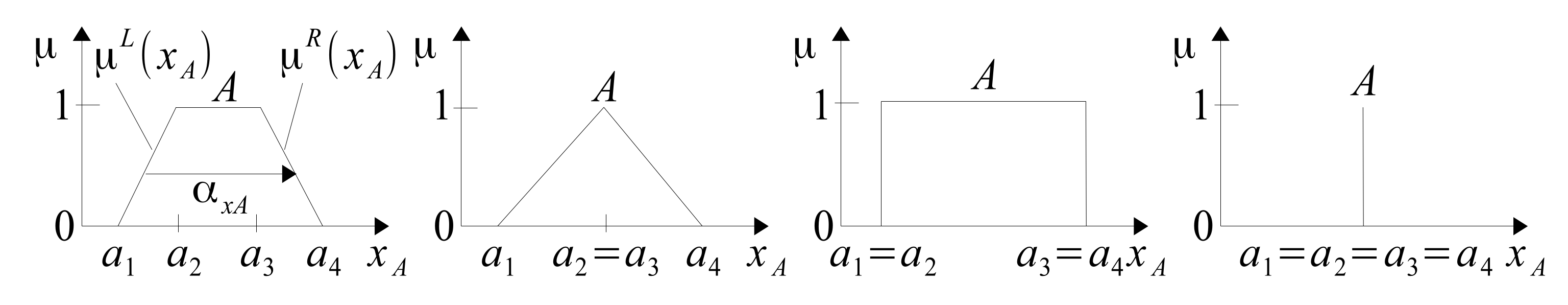As in the case of interval numbers, also in the case of fuzzy numbers T1FNs and T2FNs, sets of solutions of the results of arithmetic operations ($+,-,·,/$), solutions of equations with unknowns, etc., are multidimensional sets. Each uncertain number is a mathematical record (model) of our approximate knowledge of the true value of the variable. In F-arithmetic, we most often use trapezoidal MFs, which, on the one hand, facilitate the execution of calculations, and on the other hand, include several frequently used cases of fuzzy numbers shown in Figure 2.

Of course, other types of FNs as sinusoidal, polynomial, etc. can also be used. Classic FA uses vertical MFs. Formula (4) gives a mathematical model of the vertical trapezoidal MF from Figure 2.

$$\mu \left(x_A\right)=\left\{\begin{array}{ccc}{\mu }^L\left(x_A\right)=\frac{x_A-a_1}{a_2-a_1}\hfill & ,\hfill & a_1\le x_A\le a_2\hfill \\ 1\hfill & ,\hfill & a_2<x_A\le a_3\hfill \\ {\mu }^R\left(x_A\right)=\frac{a_4-x_A}{a_4-a_3}\hfill & ,\hfill & a_3<x_A\le a_4\hfill \end{array}\right.$$

(4)

Vertical MF is a model of only the borders of the fuzzy set and it results from the first definition of FS of Zadeh [27]. However, the vertical MF does not model the interior of an FS. In MFA, horizontal MFs are used, which model not only the borders, but also the entire interior of the MF. The HMFs correspond to (follow from) the second definition of FS Zadeh [2].

Definition 1.

A horizontal membership function type-1 $A(\mu ,{\alpha }_{xA})$ is based on a pair of functions $x_A^L\left(\mu \right)$ and $x_A^R\left(\mu \right)$, where $x_A^L\left(\mu \right)$ is left border, bounded continuous nondecreasing function over $[0,1]$ and $x_A^R\left(\mu \right)$ is right border, bounded continuous nonincreasing function over $[0,1]$. Functions $x_A^L\left(\mu \right)={\left({\mu }^L\left(x_A\right)\right)}^{-1}$ and $x_A^R\left(\mu \right)={\left({\mu }^R\left(x_A\right)\right)}^{-1}$ are horizontal representations of the left and right borders respectively, where ${\mu }^L\left(x_A\right)$ represents the left border of the vertical MF and ${\mu }^R\left(x_A\right)$ represents the right border. The type-1 horizontal multidimensional membership function type-1 (T1HMF) in general notation has the form of (5).

$$\begin{array}{c}A(\mu ,{\alpha }_{xA}):x_A(\mu ,{\alpha }_{xA})\in A(\mu ,{\alpha }_{xA})\hfill \\ x_A(\mu ,{\alpha }_{xA})=x_A^L\left(\mu \right)+{\alpha }_{xA}[x_A^R\left(\mu \right)-x_A^L\left(\mu \right)],\mu ,{\alpha }_{xA}\in [0,1]\hfill \end{array}$$

(5)

Definition 2.

Horizontal trapezoidal membership function type-1 (T1HTMF) is formulated by Equation (6),

$$A(\mu ,{\alpha }_{xA}):x_A(\mu ,{\alpha }_{xA})=[a_1+\mu (a_2-a_1)]+{\alpha }_{xA}[(a_4-a_1)-\mu (a_4-a_3+a_2-a_1)],$$

(6)

where $\mu ,{\alpha }_{xA}\in [0,1]$.

RDM means here relative-distance-measure, and can be denoted e.g., by ${\alpha }_{xA}\in [0,1]$. It defines the relative position of the point x lying between the borders of MF. For the left border ${\alpha }_{xA}=0$ and for the right border ${\alpha }_{xA}=1$. T1TMF is a mathematical model of the true value (epistemic case) of uncertain variable $x_A$ in conditions when our knowledge about this value is expressed in the form of the trapezoidal MF, Figure 2 and Figure 3.

Definition 3.

(MT1TFN-arithmetic of normal trapezoidal FNs). Let $A_1=(a_{11},a_{12},a_{13},a_{14})$ and $A_2=(a_{21},a_{22},a_{23},a_{24})$ are two arbitrary trapezoidal T1TFNs. Arithmetic operations $\odot \in \{+,-,·,/\}$ of T1FNs are defined as follows, $0\notin A_2$ for operation /.

$$\begin{array}{c}{A}_1(\mu ,{\alpha }_{x{A}_1}):x_{A_1}(\mu ,{\alpha }_{x{A}_1})\in A_1(\mu ,{\alpha }_{x{A}_1})\hfill \\ A_2(\mu ,{\alpha }_{x{A}_2}):x_{A_2}(\mu ,{\alpha }_{x{A}_2})\in A_2(\mu ,{\alpha }_{x{A}_2})\hfill \\ Z(\mu ,{\alpha }_{x{A}_1},{\alpha }_{x{A}_2})=A_1(\mu ,{\alpha }_{x{A}_1})\odot A_2(\mu ,{\alpha }_{x{A}_2})\hfill \\ Z(\mu ,{\alpha }_{x{A}_1},{\alpha }_{x{A}_2}):z(\mu ,{\alpha }_{x{A}_1},{\alpha }_{x{A}_2})\in Z(\mu ,{\alpha }_{x{A}_1},{\alpha }_{x{A}_2})\hfill \\ z(\mu ,{\alpha }_{x{A}_1},{\alpha }_{x{A}_2})=x_{A_1}(\mu ,{\alpha }_{x{A}_1})\odot x_{A_2}(\mu ,{\alpha }_{x{A}_2})\hfill \end{array}$$

(7)

For trapezoidal T1TFNs:

$$x_{A_1}(\mu ,{\alpha }_{x{A}_1})=[a_{11}+\mu (a_{12}-a_{11})]+{\alpha }_{x{A}_1}[(a_{14}-a_{11})-\mu (a_{14}-a_{13}+a_{12}-a_{11})],$$

$$x_{A_2}(\mu ,{\alpha }_{x{A}_2})=[a_{21}+\mu (a_{22}-a_{21})]+{\alpha }_{x{A}_2}[(a_{24}-a_{21})-\mu (a_{24}-a_{23}+a_{22}-a_{21})],$$

where $\mu ,{\alpha }_{x{A}_1},{\alpha }_{x{A}_2}\in [0,1]$. If T1FNs are not trapezoidal, appropriate formulas for $x_{A_1}(\mu ,{\alpha }_{x{A}_1})$ and $x_{A_2}(\mu ,{\alpha }_{x{A}_2})$ should be used.

If the support of $A_2$ contains zero, then the operation of division is of multi-granular character. This case has been described in [13].

Note that single fuzzy numbers $A_1(\mu ,{\alpha }_{x{A}_1})$ and $A_2(\mu ,{\alpha }_{x{A}_2})$ are mathematical objects in 3D space, see Figure 4. However, their result $Z(\mu ,{\alpha }_{x{A}_1},{\alpha }_{x{A}_2})=A_1(\mu ,{\alpha }_{x{A}_1})\odot A_2(\mu ,{\alpha }_{x{A}_2})$ of basic arithmetic operation $\odot \in \{+,-,·,/\}$ is a mathematical object in 4D space and cannot be visualized. Examples of arithmetic operations for T1FNs and a more detailed explanation of them can be found in articles [11,12,13,14,17].

Now, consider two T1TFNs $A_1=(1,2,3,4)$ and $A_2=(3,4,5,7)$, Figure 3. Horizontal MFs of these FNs are given by (8).

$$\begin{array}{c}{A}_1(\mu ,{\alpha }_{x{A}_1}):x_{A_1}(\mu ,{\alpha }_{x{A}_1})\in A_1(\mu ,{\alpha }_{x{A}_1});x_{A_1}(\mu ,{\alpha }_{x{A}_1})=(1+\mu )+{\alpha }_{x{A}_1}(3-2\mu )\hfill \\ A_2(\mu ,{\alpha }_{x{A}_2}):x_{A_2}(\mu ,{\alpha }_{x{A}_2})\in A_2(\mu ,{\alpha }_{x{A}_2});x_{A_2}(\mu ,{\alpha }_{x{A}_2})=(3+\mu )+{\alpha }_{x{A}_2}(4-3\mu )\hfill \\ \mu ,{\alpha }_{x{A}_1},{\alpha }_{x{A}_2}\in [0,1]\hfill \end{array}$$

(8)

Note that $x_{A_1}=f_{A_1}(\mu ,{\alpha }_{x{A}_1})$ and $x_{A_2}=f_{A_2}(\mu ,{\alpha }_{x{A}_2})$ are not 2D but 3D mathematical objects. Figure 3 illustrates the sense of the horizontal number models $A_1$ and $A_2$ in 2D space ($M\times X_{A_1}$, $M\times X_{A_2}$).

HMF in Figure 3 models in 2D space the entire surface inside the HMF. The 2D space $M\times X_{A_1}$ is not the full space of this function, but only a subspace, because this function exists in the 3D space $M\times X_{A_1}\times A_{x{A}_1}$, as shown in Figure 4.

The realization of the multiplication $A_1·A_2$ is given by the Formula (9).

$$\begin{array}{c}Z=A_1·A_2,Z:z\in Z\hfill \\ Z(\mu ,{\alpha }_{x{A}_1},{\alpha }_{x{A}_2})=A_1(\mu ,{\alpha }_{x{A}_1})·A_2(\mu ,{\alpha }_{x{A}_2})\hfill \\ Z(\mu ,{\alpha }_{x{A}_1},{\alpha }_{x{A}_2}):z(\mu ,{\alpha }_{x{A}_1},{\alpha }_{x{A}_2})\in Z(\mu ,{\alpha }_{x{A}_1},{\alpha }_{x{A}_2})\hfill \\ z(\mu ,{\alpha }_{x{A}_1},{\alpha }_{x{A}_2})=x_{A_1}(\mu ,{\alpha }_{x{A}_1})·x_{A_2}(\mu ,{\alpha }_{x{A}_2})\hfill \\ z(\mu ,{\alpha }_{x{A}_1},{\alpha }_{x{A}_2})=[(1+\mu )+{\alpha }_{x{A}_1}(3-2\mu )]·[(3+\mu )+{\alpha }_{x{A}_2}(4-3\mu )]\hfill \\ \mu ,{\alpha }_{x{A}_1},{\alpha }_{x{A}_2}\in [0,1]\hfill \end{array}$$

(9)

The algebraic and universal result of the multiplication Z being the set of quadruples $(\mu ,{\alpha }_{x{A}_1},{\alpha }_{x{A}_2},z)$ exists in 4D space and cannot be seen. Instead, you can define its span $S{P}_Z$ in the direction of the z axis and see it in 2D space $Z\times M$. The span $S{P}_Z$ of the multiplication result Z is given by the Formula (10) and Figure 5.

$$\begin{array}{c}S{P}_Z\left(\mu \right)=[\underset{{\alpha }_{x{A}_1},{\alpha }_{x{A}_2}}{min}z(\mu ,{\alpha }_{x{A}_1},{\alpha }_{x{A}_2}),\underset{{\alpha }_{x{A}_1},{\alpha }_{x{A}_2}}{max}z(\mu ,{\alpha }_{x{A}_1},{\alpha }_{x{A}_2})]\hfill \\ \mu ,{\alpha }_{x{A}_1},{\alpha }_{x{A}_2}\in [0,1]\hfill \end{array}$$

(10)

The examination of the function (9) shows that its minimum border is obtained for ${\alpha }_{x{A}_1}={\alpha }_{x{A}_2}=0$ and the maximum border for ${\alpha }_{x{A}_1}={\alpha }_{x{A}_2}=1$.

The mathematical properties of MF arithmetic are described and proven in [42]. The following properties hold in type 1 multidimensional epistemic fuzzy arithmetic:

-

addition and multiplication of MFNs are commutative and associative,

-

there exist neutral elements of addition and multiplication,

-

there exist an additive and multiplicative inverse elements,

-

the distributive law holds,

-

the cancellation laws for addition and multiplication hold,

-

the result of arithmetic operations is multidimensional,

-

in MFA, the result of arithmetic operations is universal, it does not depend on the mathematical form of the problem.

Denotation principle of epistemic fuzzy numbers

Each FN occurring in the problem is usually marked with a letter symbol, e.g., X or A. One letter symbol, e.g., A can usually be used only to denote one fuzzy number, because this number is a record of our knowledge about only one true value (although unknown exactly) of the variable a, e.g., an uncertain amount of water in the tank. Even if our knowledge of the value of the second variable b has the form of an identical fuzzy number, the real values of the variables a and b are likely to differ. The mathematical equality $A=B$ does not necessarily mean that $a=b$. Unless we have such knowledge. Usually when $A=B$, there is no $a=b$, but $a\ne b$.

3. Border and Body Definition of T2FS

The concept of a type 1 fuzzy set was introduced by Zadeh in 1965 in [27]. A T1FS A on the universe of discourse X is characterized by its membership function ${\mu }_A\left(x\right)$ and represented as follows (11), Mendel [43].

$$A=\left\{(x,{\mu }_A\left(x\right))\right|\forall x\in X,{\mu }_A\left(x\right)\in [0,1]\}$$

(11)

where X—universe of discourse, ${\mu }_A$—membership function.

As the left and right border of MF ${\mu }_A\left(x\right)$ are sometimes difficult to identify accurately, there is some uncertainty about their position. This is why L. Zadeh, in 1975, in [2], introduced the concept of T2FS. However, this original definition of T2FS was a little vague, which prompted attempts to refine it, as well as giving different interpretations of T2FS. Some scientific confusion has arisen. Therefore, J.M. Mendel, M.R. Rajati and P. Susner proposed the ordering of this definition in [43,44]. In this ordered definition, X is the universe of discourse for primary variable x and U for the secondary variable $u\in [0,1]$. A T2FS denoted $\tilde{A}$ is determined by a T2MF ${\mu }_{\tilde{A}}(x,u)$, where x belongs to X and u belongs to U (12).

$$\tilde{A}=\left\{((x,u),{\mu }_{\tilde{A}}(x,u))\right|x\in X,u\in [0,1]\}$$

(12)

In the current definition (12) of T2FS, the primary membership $J_x$ does not occur, Equation (13).

$$J_x=\left\{(x,u)\right|u\in [0,1],{\mu }_{\tilde{A}}(x,u)>0\}$$

(13)

The set $\tilde{A}$ can also be expressed [44] in a special fuzzy notation (14).

$$\tilde{A}=\underset{x\in X}{\int }\underset{u\in [0,1]}{\int }{\mu }_{\tilde{A}}(x,u)/(x,u)$$

(14)

The symbol ∫ denotes here union over all admissible values of x and u. In definition of $\tilde{A}$, the concept of secondary MF [43] is used (15).

$${\mu }_{\tilde{A}\left(x\right)}\left(u\right)=\underset{u\in [0,1]}{\int }{\mu }_{\tilde{A}}(x,u)/u=\underset{u\in [0,1]}{\int }{f}_x\left(u\right)/u$$

(15)

$\tilde{A}\left(x\right)$ is a T1FS which is referred to as a secondary set. It can be represented by its $\alpha$-cut decomposition. $\left\{{\mu }_{\tilde{A}}\left(u\right)\right|u\in U\}$ can be called vertical slice of ${\mu }_{\tilde{A}}(x,u)$. In the updated border definition of T2FS, the concept of footprint of uncertainty ($FOU$) can be used further (16).

$$FOU\left(\tilde{A}\right)=\left\{(x,u)\right|x\in X\mathrm{and}u\in [{\underline{\mu }}_{\tilde{A}}\left(x\right),{\overline{\mu }}_{\tilde{A}}\left(x\right)]\}$$

(16)

In Formula (16), ${\underline{\mu }}_{\tilde{A}}\left(x\right)$ means lower MF (LMF) and ${\overline{\mu }}_{\tilde{A}}\left(x\right)$ means upper MF (UMF) [44]. The MFs are given by (17) and (18).

$${\underline{\mu }}_{\tilde{A}}\left(x\right)=inf\left\{u\right|u\in [0,1],{\mu }_{\tilde{A}}(x,u)>0\}$$

(17)

$${\overline{\mu }}_{\tilde{A}}\left(x\right)=sup\left\{u\right|u\in [0,1],{\mu }_{\tilde{A}}(x,u)>0\}$$

(18)

A special type of T2FS is the interval T2FS (IT2FS) defined by (19), where all secondary grades ${\mu }_{\tilde{A}}(x,u)=1$.

$$\tilde{A}=\left\{((x,u),{\mu }_{\tilde{A}}(x,u)=1)\right|\forall x\in X,\forall u\in J_x\subseteq [0,1]\}$$

(19)

Visualization of a triangular T2FS is shown in Figure 6.

Figure 6 clearly shows the border nature of the current definition of T2FS, which defines only the left and right border of this set. The first definition of T1FS by Zadeh from [27] has the same boundary character. Figure 7 shows an example of a triangular MF defining a T1FS.

In addition to the border definition of T1FS, Zadeh also published a second, less known definition of this set [2] based on $\alpha$-cuts called $\alpha$-level sets by him. This definition is readily used in FA.

If A is a fuzzy set of X, then $\alpha$-level set of A is a nonfuzzy set denoted by $A_{\alpha }$, which comprises all elements of X whose grade $\mu$ of membership in A is greater or equal to $\alpha$. In symbols

$$A_{\alpha }=\left\{x\right|{\mu }_A\left(x\right)\ge \alpha \}$$

(20)

A fuzzy set A may be decomposed into level sets through the resolution identity (21) or (22).

$$A=\underset{0}{\overset{1}{\int }}\alpha A_{\alpha }$$

(21)

or

$$A=\sum _{\alpha }\alpha A_{\alpha }$$

(22)

where $\alpha A_{\alpha }$ is the product of a scalar $\alpha$ with the set $A_{\alpha }$ in the sense $A={\mu }_1{x}_1+\dots +{\mu }_n{x}_n$ or $A={\displaystyle \sum _{i=1}^n}{\mu }_i{x}_i$ and $\underset{0}{\overset{1}{\int }}$ (or ${\displaystyle \sum _{\alpha }}$) is the union of the $A_{\alpha }$ with $\alpha$ ranging from 0 to 1.

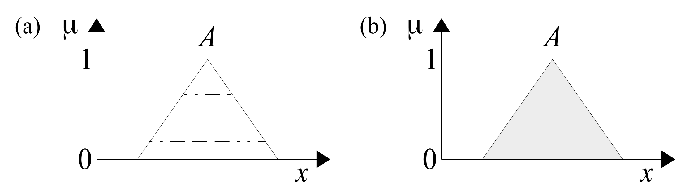
If fuzzy set A can be decomposed into a set of $\alpha$-levels-set $A_{\alpha }$, then the inverse operations, composing A of $A_{\alpha }$-s is also possible. This possibility is illustrated in Figure 8.

In the horizontal definition (21) of a T1FS, Zadeh determines the set not only by the MF ${\mu }_A\left(x\right)$, as in (20), but also by all sets $A_{\alpha }$ lying within the MF ${\mu }_A\left(x\right)$, i.e., also by interior (body) of this function. Hence, this definition can be called body definition of a T1FS. Instead, the first, vertical definition (11) can be called the border one. A new, horizontal definition of T2FS will be briefly presented below. This definition was presented earlier in 2019 in [40]. In Figure 9, a trapezoidal MF representing a certain fuzzy concept of A is shown.

MF-core is an interval containing those x-values that are most consistent with the sense of the fuzzy concept A. On the other hand, MF-support includes all values of x that fully or at least partially, to the degree ${\mu }_A$, comply with the sense of this concept. The negation of the support of A consists of those values of the variable x, which do not have any, even minimal compliance with the concept A.

In the case of T2FS $\tilde{A}$, there is uncertainty, not only as to the degree of membership ${\mu }_{\tilde{A}}$ of individual values of x to the T2FS, but also as regards the membership function to the set A itself, and more specifically, the uncertainty about the position of the function borders (left) ${\mu }_{\tilde{A}}^L$ and (right) ${\mu }_{\tilde{A}}^R$. This uncertainty arises, e.g., during the MF identification experiment based on the opinions of many experts. If we ask experts to identify their own individual T1MFs of some fuzzy concept (e.g., evaluating the value of a used car of a certain brand), the T1MFs given by these experts will usually differ from each other. Their left and right borders will be different. An example of the possible distribution of expert judgments is presented in Figure 10.

There is a need to generalize all individual expert evaluations and present them in the form of a possibly concise representative evaluation. Such a generalized, concise representation can be the outer and inner T1MF. Internal T1MF ${\mu }_{in}\left(x\right)$ can be interpreted as the most reliable T1MF representing all individual expert evaluations. Therefore, it can be assigned a confidence grade of $c=1$. On the other hand, the outer ${\mu }_{out}\left(x\right)$ can be assigned a confidence grade of $c=0$, in the sense that it is for each level of membership $\mu$ the border, outside of which there are no longer any x values that would belong to the fuzzy concept. Outside of ${\mu }_{out}\left(x\right)$, there is only a non-membership zone to the concept. Outer and inner T1MFs, taken together, can be interpreted as FOU of T2FS, as a set whose borders are uncertain. The outer T1MF ${\mu }_{out}\left(x\right)$ can be interpreted as support-T1MF and the inner ${\mu }_{in}\left(x\right)$ as core-T1MF of a T2MF. The border uncertainty zones of the T2MF can be interpreted as transition zones, i.e., the transition zones ${\mu }_{out}\left(x\right)$ into ${\mu }_{in}\left(x\right)$, i.e., the transformation of support-T1MF into core-T1MF. Core-T1MF can be normal T1MF ($max\mu \left(x\right)=1$) or not-normal T1MF ($max\mu \left(x\right)<1$). 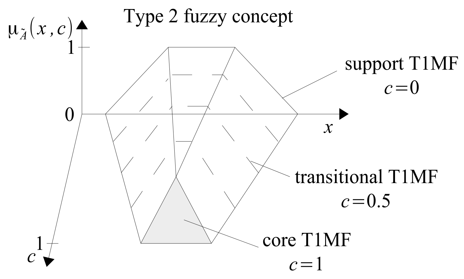In this article, we will only cover normal T2FS having normal support-T1MF and normal core-T1MF. In the case of both support-MFs and core-MFs, we will deal with triangular and trapezoidal MFs. 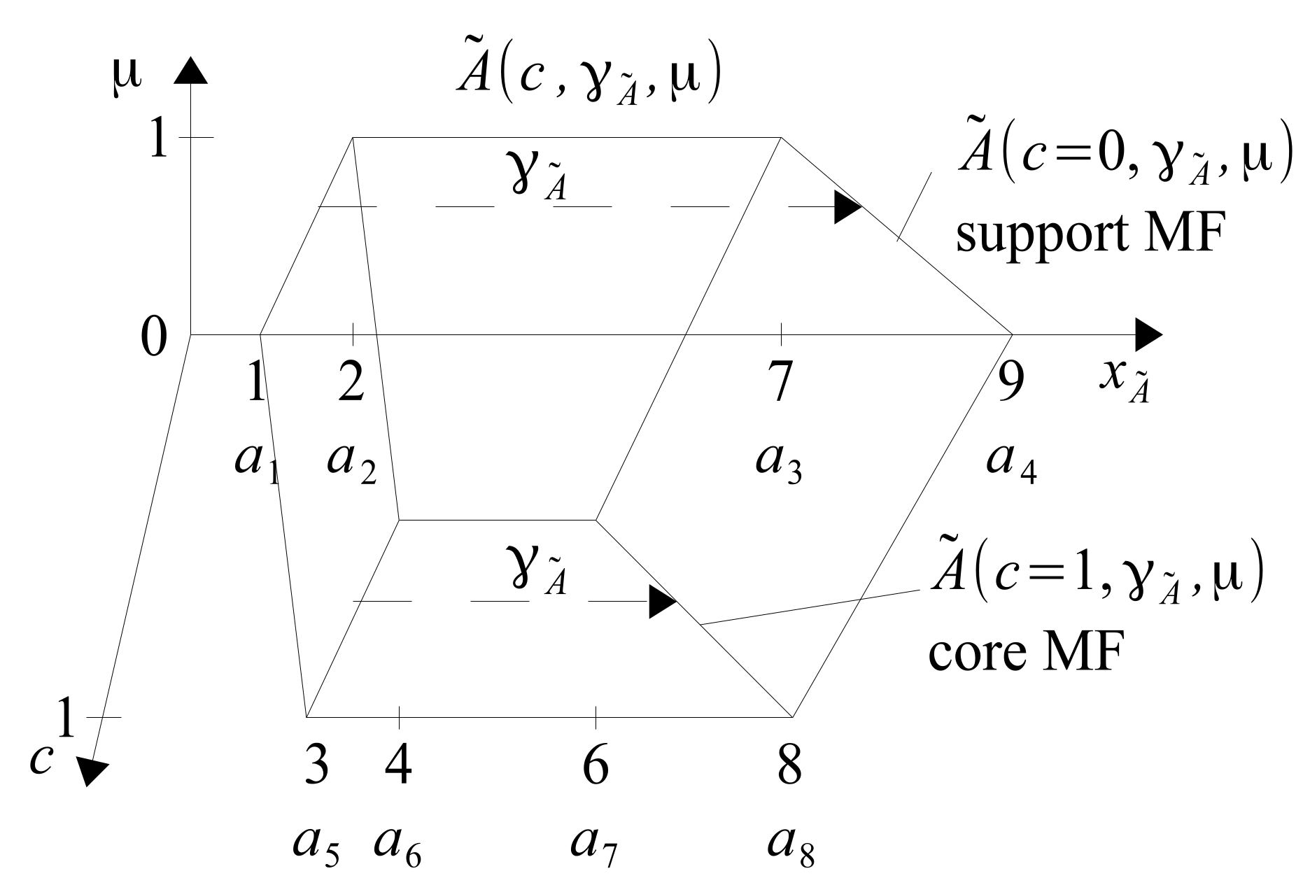An example of a FOU of T2MF with a trapezoidal support-T1MF and a triangular core-T1MF is shown in Figure 11.

Confidence degree c is the third variable characterizing T2FS, which means that T2MF is a set in 3D space, as shown in Figure 12.

The T2MF shown in Figure 12 can be interpreted as a transition function of support-T1MF into core-T1MF. T1MFs in between may be called transitional T1MFs. Transition can be linear or non-linear. It depends on the nature of the experts’-T1MFs’ distribution from which their T2MF representation is identified. However, the identification of the type of transition is not the subject of this article and requires a separate study. In this article, a linear transition will be assumed, as is the case with the most commonly used trapezoidal T1MFs, Figure 9, where the membership function can be interpreted as a linear transition of the support interval in the core interval. If T2MF represents only 2 expert opinions, then rather a linear transition should be assumed. If the number of expert T1MFs (Figure 10) is higher, the type of transition can be identified. Similar methods can be developed here, as presented, e.g., in [45,46], to identify the current version of T2MF defined by the Formula (12).

There are two types of MFs related to T2FS $\tilde{A}$. The first type of this function is the function which will be denoted as ${\mu }_{out}\left(x\right)$ and conventionally will be called vertical. This function is a mathematical model of the outer shell of the geometric figure shown in Figure 12. It corresponds to the first Zadeh’s definition of T1MF defined by (11); an example is given in Figure 7.

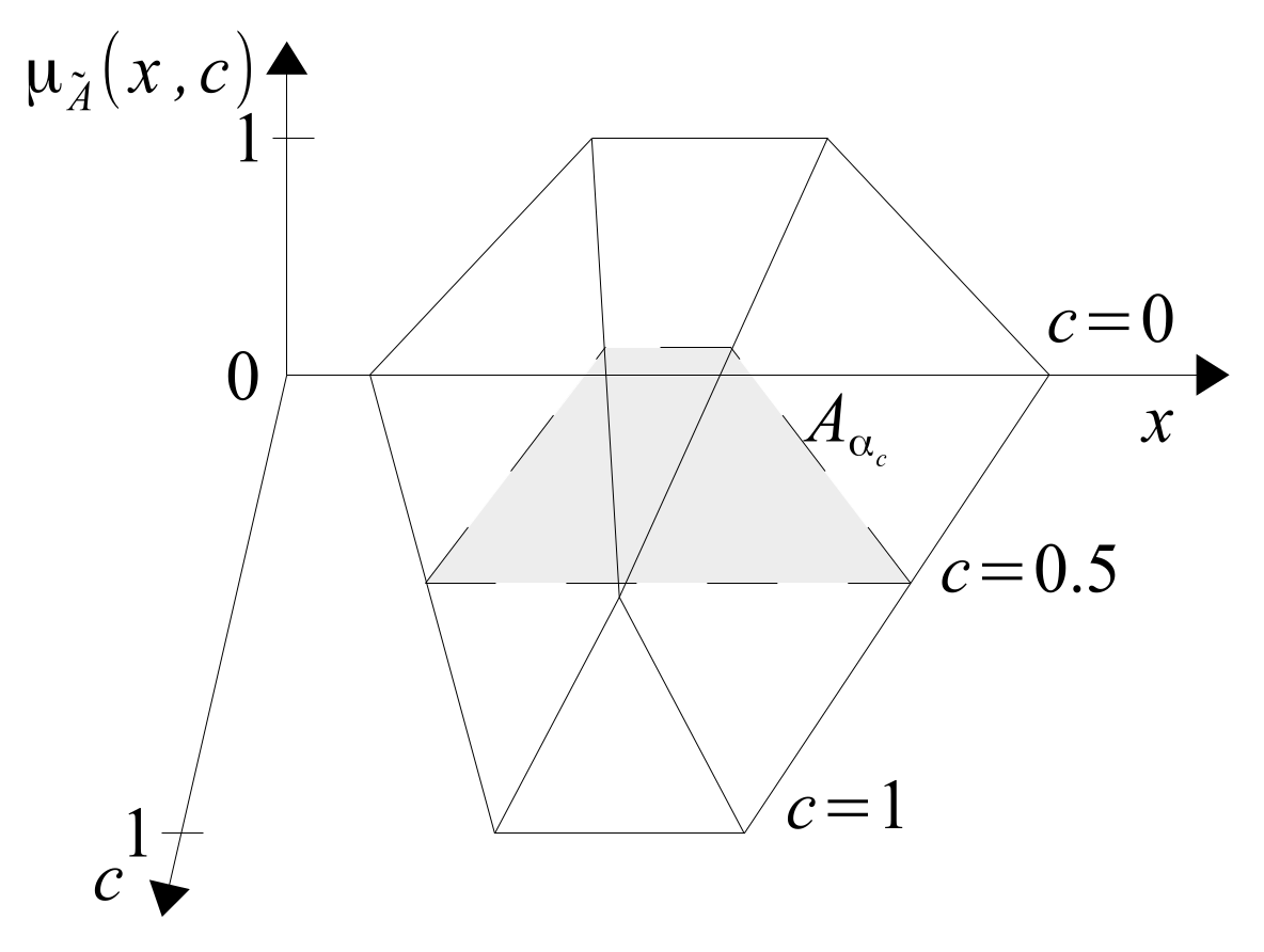
The second type of T2MF is a function that will be conventionally called body-T2MF because it is composed of ${\alpha }_c$-cuts (cuts made at the level ${\alpha }_c$ of the full 3D MF ${\mu }_{\tilde{A}}(x,c)$, see Figure 13.

The body-T2MF is an analogy to the second Zadeh’s definition of T1MF given by Formulas (20) and (21) and illustrated in Figure 10. Body-T2MF defines not only the outer shell of the T2FS in Figure 12, but also the whole of its interior, i.e., the whole body of it. A T2F-set $\tilde{A}$ can be composed of ${\alpha }_c$-cuts respectively for continuous (23) and discrete sets (24).

$$\tilde{A}=\underset{0}{\overset{1}{\int }}{\alpha }_c{A}_{{\alpha }_c}$$

(23)

$$\tilde{A}=\sum _{{\alpha }_c}{\alpha }_c{A}_{{\alpha }_c}$$

(24)

The cut $A_{{\alpha }_c}$ is defined by Formula (25) [43].

$$A_{{\alpha }_c}=\left\{x\right|{\mu }_{\tilde{A}}\left(x\right)\ge {\alpha }_c\}$$

(25)

$A_{{\alpha }_c}$-cuts are very useful. They allow for simple implementations of arithmetic calculations on T2FNs by decomposing them into calculations with T1FNs.

4. Multidimensional, Epistemic Fuzzy Arithmetic of Type-2 Fuzzy Numbers

MET2F-arithmetic is more difficult and complex than MET1FA. This is due to the fact that the dimensionality of T2FN is higher than that of T1FN. For this reason, an increase in the calculation complexity is understandable. The general definition of multidimensional epistemic type-2 fuzzy number is given as follows.

Definition 4.

Multidimensional epistemic type 2 fuzzy number $\tilde{A}$ in horizontal notation has a form of (26)

$$\begin{array}{c}\tilde{A}(c,{\gamma }_{\tilde{A}},\mu ):x_{\tilde{A}}(c,{\gamma }_{\tilde{A}},\mu )\in \tilde{A}(c,{\gamma }_{\tilde{A}},\mu )\hfill \\ x_{\tilde{A}}(c,{\gamma }_{\tilde{A}},\mu )=x_{\tilde{A}}^{supp}(c=0,{\gamma }_{\tilde{A}},\mu )+c[x_{\tilde{A}}^{core}(c=1,{\gamma }_{\tilde{A}},\mu )-x_{\tilde{A}}^{supp}(c=0,{\gamma }_{\tilde{A}},\mu )],\hfill \\ c,{\gamma }_{\tilde{A}},\mu \in [0,1],\hfill \end{array}$$

(26)

where $x_{\tilde{A}}^{supp}(c=0,{\gamma }_{\tilde{A}},\mu )$ and $x_{\tilde{A}}^{core}(c=1,{\gamma }_{\tilde{A}},\mu )$ are the support and core of a fuzzy number type 2 and have a horizontal fuzzy number notation of the form (27).

$$\begin{array}{c}{x}_{\tilde{A}}^{supp}(c=0,{\gamma }_{\tilde{A}},\mu )=x_{\tilde{A}}^L\left(\mu \right)+{\gamma }_{\tilde{A}}[x_{\tilde{A}}^R\left(\mu \right)-x_{\tilde{A}}^L\left(\mu \right)],\mu ,{\gamma }_{\tilde{A}}\in [0,1],\hfill \\ x_{\tilde{A}}^{core}(c=1,{\gamma }_{\tilde{A}},\mu )=x_{\tilde{A}}^L\left(\mu \right)+{\gamma }_{\tilde{A}}[x_{\tilde{A}}^R\left(\mu \right)-x_{\tilde{A}}^L\left(\mu \right)],\mu ,{\gamma }_{\tilde{A}}\in [0,1],\hfill \end{array}$$

(27)

where $x_{\tilde{A}}^L\left(\mu \right)$ is left border, bounded continuous nondecreasing function over $[0,1]$, while $x_{\tilde{A}}^R\left(\mu \right)$ is right border, bounded continuous nonincreasing functions over $[0,1]$.

The complexity of calculations cannot be avoided. However, MET2FA operations are not extremely difficult because they can be decomposed into MET1FA operations, just as MET1FA operations can be decomposed into interval arithmetic (MET0FA) operations. The realization of MET2FA operations will be explained using two T2FNs $\tilde{A}$ and $\tilde{B}$, which are shown in Figure 14, Figure 15, Figure 16 and Figure 17. Both the letters and the assumed numerical values of the individual parameters are given in these figures.

The number $\tilde{A}$ with Definition 4 is given by the general Formula (28) and its components by the Formulas (29) and (30). Denotation $\tilde{A}(c,{\gamma }_{\tilde{A}},\mu )$ concerns the set of all possible values of the variable $x_{\tilde{A}}$ belonging to the set $\tilde{A}$, whereas the denotation $x_{\tilde{A}}$ concerns a single numerical value contained in the set $\tilde{A}$.

$$\tilde{A}(c,{\gamma }_{\tilde{A}},\mu ):x_{\tilde{A}}(c,{\gamma }_{\tilde{A}},\mu )=x_{\tilde{A}}(c=0,{\gamma }_{\tilde{A}},\mu )+c[x_{\tilde{A}}(c=1,{\gamma }_{\tilde{A}},\mu )-x_{\tilde{A}}(c=0,{\gamma }_{\tilde{A}},\mu )],c,{\gamma }_{\tilde{A}},\mu \in [0,1]$$

(28)

$$\tilde{A}(c=0,{\gamma }_{\tilde{A}},\mu ):x_{\tilde{A}}(c=0,{\gamma }_{\tilde{A}},\mu )=[a_1+\mu (a_2-a_1)]+{\gamma }_{\tilde{A}}\{[a_4-\mu (a_4-a_3)]-[a_1+\mu (a_2-a_1)]\},{\gamma }_{\tilde{A}},\mu \in [0,1]$$

(29)

$$\tilde{A}(c=1,{\gamma }_{\tilde{A}},\mu ):x_{\tilde{A}}(c=1,{\gamma }_{\tilde{A}},\mu )=[a_5+\mu (a_6-a_5)]+{\gamma }_{\tilde{A}}\{[a_8-\mu (a_8-a_7)]-[a_5+\mu (a_6-a_5)]\},{\gamma }_{\tilde{A}},\mu \in [0,1]$$

(30)

Formulas (28)–(30) seem quite complex. However, after inserting the numerical values of individual parameters into them, they obtain a fairly simple form (31).

$$\tilde{A}(c,{\gamma }_{\tilde{A}},\mu ):x_{\tilde{A}}(c,{\gamma }_{\tilde{A}},\mu )=(1+\mu +2c)+{\gamma }_{\tilde{A}}(8-3\mu -3c),c,{\gamma }_{\tilde{A}},\mu \in [0,1]$$

(31)

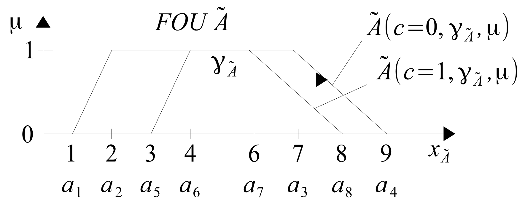
Figure 16 shows the number $\tilde{B}$ in full 3D space and Figure 17 shows the FOU $\tilde{B}$. By contrast, the number $\tilde{B}$ has a triangular and not a trapezoidal core-$\tilde{B}(c=1,{\gamma }_{\tilde{B}},\mu )$.

It is easy to see that there is no special need to represent the T2FNs in the form of 3-dimensional figures. Presenting these numbers in the form of 2D-FOUs is sufficient. If the support-T1MF transition in core-T1MF is linear, it is enough to show only 2 cuts. If the transition is non-linear, 3 or more cuts of 3D-T2MF can be shown. The number $\tilde{B}$ with Definition 4 is given by the general Formula (32) and its constituent elements by the Formulas (33) and (34).

$$\tilde{B}(c,{\gamma }_{\tilde{B}},\mu ):x_{\tilde{B}}(c,{\gamma }_{\tilde{B}},\mu )=x_{\tilde{B}}(c=0,{\gamma }_{\tilde{B}},\mu )+c[x_{\tilde{B}}(c=1,{\gamma }_{\tilde{B}},\mu )-x_{\tilde{B}}(c=0,{\gamma }_{\tilde{B}},\mu )],c,{\gamma }_{\tilde{B}},\mu \in [0,1]$$

(32)

$$\tilde{B}(c=0,{\gamma }_{\tilde{B}},\mu ):x_{\tilde{B}}(c=0,{\gamma }_{\tilde{B}},\mu )=[b_1+\mu (b_2-b_1)]+{\gamma }_{\tilde{B}}\{[b_4-\mu (b_4-b_3)]-[b_1+\mu (b_2-b_1)]\},{\gamma }_{\tilde{B}},\mu \in [0,1]$$

(33)

$$\tilde{B}(c=1,{\gamma }_{\tilde{B}},\mu ):x_{\tilde{B}}(c=1,{\gamma }_{\tilde{B}},\mu )=[b_5+\mu (b_6-b_5)]+{\gamma }_{\tilde{B}}\{[b_8-\mu (b_8-b_7)]-[b_5+\mu (b_6-b_5)]\},{\gamma }_{\tilde{B}},\mu \in [0,1]$$

(34)

$$\tilde{B}(c,{\gamma }_{\tilde{B}},\mu ):x_{\tilde{B}}(c,{\gamma }_{\tilde{B}},\mu )=(10+3\mu +3c-c\mu )+{\gamma }_{\tilde{B}}(11-7\mu -7c+3c\mu ),c,{\gamma }_{\tilde{B}},\mu \in [0,1]$$

(35)

Adding T2FNs

For the assumed numbers $\tilde{A}$, Formulas (28) and (31) and $\tilde{B}$, Formulas (32) and (35), the result $\tilde{C}$ of addition is given by the Formula (36).

$$\begin{array}{c}\tilde{A}(c,{\gamma }_{\tilde{A}},\mu )+\tilde{B}(c,{\gamma }_{\tilde{B}},\mu )=\tilde{C}(c,{\gamma }_{\tilde{A}},{\gamma }_{\tilde{B}},\mu ):x_{\tilde{A}}(c,{\gamma }_{\tilde{A}},\mu )+x_{\tilde{B}}(c,{\gamma }_{\tilde{B}},\mu )=x_{\tilde{C}}(c,{\gamma }_{\tilde{A}},{\gamma }_{\tilde{B}},\mu ),c,{\gamma }_{\tilde{A}},{\gamma }_{\tilde{B}},\mu \in [0,1]\hfill \\ x_{\tilde{C}}(c,{\gamma }_{\tilde{A}},{\gamma }_{\tilde{B}},\mu )=[(1+\mu +2c)+{\gamma }_{\tilde{A}}(8-3\mu -3c)]+[(10+3\mu +3c-c\mu )+{\gamma }_{\tilde{B}}(11-7\mu -7c+3c\mu )]\hfill \end{array}$$

(36)

As can be seen from (36), the result $x_{\tilde{C}}(c,{\gamma }_{\tilde{A}},{\gamma }_{\tilde{B}},\mu )$ exists in 5D space, ${\gamma }_{\tilde{A}}$ corresponds to $x_{\tilde{A}}$ here, ${\gamma }_{\tilde{B}}$ corresponds to $x_{\tilde{B}}$. The 5D result cannot be seen. However, you can see simplified information about it in a 2D or 3D space, such as its span, cardinality distribution, or gravity center. However, fuzzy systems specialists are most often interested in the horizontal uncertainty of the calculated results in the form of span. In the case of a 5D-result $\tilde{C}=\tilde{A}+\tilde{B}$, its span can be determined from the Formula (37).

$$S{P}_{\tilde{C}=\tilde{A}+\tilde{B}}=[\underset{{\gamma }_{\tilde{A}},{\gamma }_{\tilde{B}}}{min}{x}_{\tilde{C}}(c,{\gamma }_{\tilde{A}},{\gamma }_{\tilde{B}},\mu ),\underset{{\gamma }_{\tilde{A}},{\gamma }_{\tilde{B}}}{max}{x}_{\tilde{C}}(c,{\gamma }_{\tilde{A}},{\gamma }_{\tilde{B}},\mu )]$$

(37)

Examination of the function $x_{\tilde{C}}(c,{\gamma }_{\tilde{A}},{\gamma }_{\tilde{B}},\mu )$, Formula (37) shows that $min{x}_{\tilde{C}}$ is obtained for ${\gamma }_{\tilde{A}}={\gamma }_{\tilde{B}}=0$ and $max{x}_{\tilde{C}}$ for ${\gamma }_{\tilde{A}}={\gamma }_{\tilde{B}}=1$. As a result, we obtain the span $S{P}_{\tilde{C}}$ defined by the Formula (38).

$$S{P}_{\tilde{C}=\tilde{A}+\tilde{B}}=[(11+4\mu +5c-c\mu ),(30-6\mu -5c+2c\mu )]$$

(38)

Figure 18 shows the visualization of the span function $S{P}_{\tilde{C}=\tilde{A}+\tilde{B}}$.

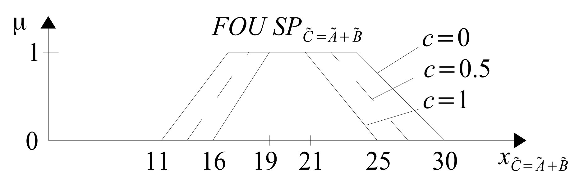
Span $S{P}_{\tilde{C}=\tilde{A}+\tilde{B}}$ does not need to be visualized in 3D space. It can be more easily presented in 2D space in the form of cuts made for various c-values entered into the Formula (38), e.g., for values $c=0$, $c=0.5$, $c=1$. We then obtain the $FOUS{P}_{\tilde{C}=\tilde{A}+\tilde{B}}$ shown in Figure 19.

It should be remembered that $FOUS{P}_{\tilde{C}=\tilde{A}+\tilde{B}}$ is not the algebraic and universal result of adding $\tilde{A}+\tilde{B}$, i.e., that equation $\tilde{A}+\tilde{B}=FOUS{P}_{\tilde{C}=\tilde{A}+\tilde{B}}$ is not satisfied as suggest low dimensional fuzzy arithmetic types. Moreover, it can easily be checked that: $\tilde{A}\ne FOUS{P}_{\tilde{C}=\tilde{A}+\tilde{B}}-\tilde{B}$ and $\tilde{B}\ne FOUS{P}_{\tilde{C}=\tilde{A}+\tilde{B}}-\tilde{A}$. The algebraic and universal result of adding $\tilde{A}+\tilde{B}$ is only the 5D number $\tilde{C}$ defined by the Formula (37). Only the number $\tilde{C}$ satisfies all possible, alternative equalities $\tilde{A}=\tilde{C}-\tilde{B}$, $\tilde{B}=\tilde{C}-\tilde{A}$, and $\tilde{A}+\tilde{B}-\tilde{C}=0$.

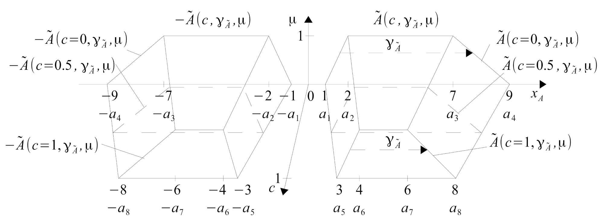
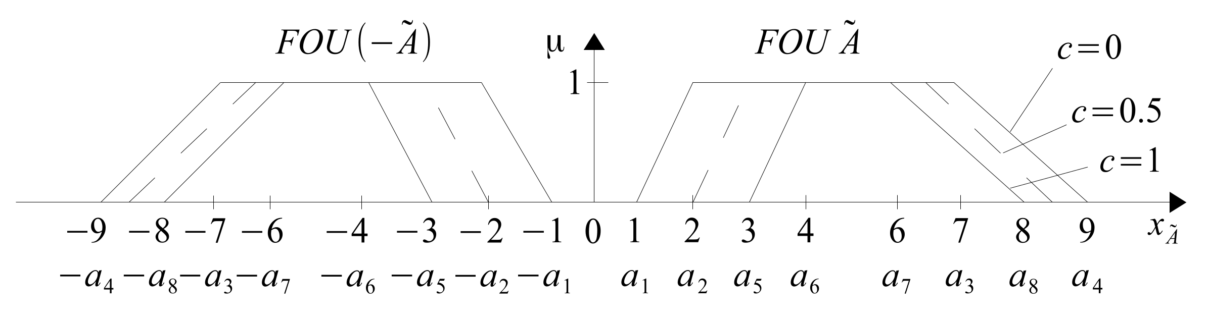
Negative type 2 fuzzy number $-\tilde{\mathbf{A}}$

T2FN $\tilde{A}$ is given by the general Formula (28). The components of the number $\tilde{A}$ are given by the Formulas (29) and (30). Hence, the specific number $\tilde{A}$ is expressed by Formula (31).

The negative fuzzy number $-\tilde{A}$ in its general form is given by the Formula (39), and its specific version by the Formula (40).

$$-\tilde{A}(c,{\gamma }_{\tilde{A}},\mu ):x_{-\tilde{A}}(c,{\gamma }_{\tilde{A}},\mu )=-x_{\tilde{A}}(c=0,{\gamma }_{\tilde{A}},\mu )-c[x_{\tilde{A}}(c=1,{\gamma }_{\tilde{A}},\mu )-x_{\tilde{A}}(c=0,{\gamma }_{\tilde{A}},\mu )],c,{\gamma }_{\tilde{A}},\mu \in [0,1]$$

(39)

$$-\tilde{A}(c,{\gamma }_{\tilde{A}},\mu ):x_{-\tilde{A}}(c,{\gamma }_{\tilde{A}},\mu )=-(1+\mu +2c)-{\gamma }_{\tilde{A}}(8-3\mu -3c),c,{\gamma }_{\tilde{A}},\mu \in [0,1]$$

(40)

Figure 20 shows T2FN $\tilde{A}$ and its negative version in 3D space and Figure 21 shows cuts of $\tilde{A}$ and $-\tilde{A}$ in the form of $FOU\tilde{A}$ and $FOU(-\tilde{A})$.

Inverse type 2 fuzzy number

T2FN $\tilde{A}$ is determined by general Formula (41) and its specific triangular version is given by (42), $0\notin \tilde{A}$.

$$\tilde{A}(c,{\gamma }_{\tilde{A}},\mu ):x_{\tilde{A}}(c,{\gamma }_{\tilde{A}},\mu )=x_{\tilde{A}}(c=0,{\gamma }_{\tilde{A}},\mu )+c[x_{\tilde{A}}(c=1,{\gamma }_{\tilde{A}},\mu )-x_{\tilde{A}}(c=0,{\gamma }_{\tilde{A}},\mu )],c,{\gamma }_{\tilde{A}},\mu \in [0,1]$$

(41)

$$\tilde{A}(c,{\gamma }_{\tilde{A}},\mu ):x_{\tilde{A}}(c,{\gamma }_{\tilde{A}},\mu )=(1+3\mu +2c-2c\mu )+{\gamma }_{\tilde{A}}(5-5\mu -3c+3c\mu ),c,{\gamma }_{\tilde{A}},\mu \in [0,1]$$

(42)

Inverse T2FN ${\tilde{A}}^{-1}$ is determined by general Formula (43) and its specific version by (44).

$$\begin{array}{c}{\tilde{A}}^{-1}(c,{\gamma }_{\tilde{A}},\mu ):x_{{\tilde{A}}^{-1}}(c,{\gamma }_{\tilde{A}},\mu )\in {\tilde{A}}^{-1}(c,{\gamma }_{\tilde{A}},\mu )\hfill \\ x_{{\tilde{A}}^{-1}}(c,{\gamma }_{\tilde{A}},\mu )={\left(x_{\tilde{A}}(c=0,{\gamma }_{\tilde{A}},\mu )\right)}^{-1}+c[{\left(x_{\tilde{A}}(c=1,{\gamma }_{\tilde{A}},\mu )\right)}^{-1}-{\left(x_{\tilde{A}}(c=0,{\gamma }_{\tilde{A}},\mu )\right)}^{-1}],c,{\gamma }_{\tilde{A}},\mu \in [0,1]\hfill \end{array}$$

(43)

$$\begin{array}{c}{\tilde{A}}^{-1}(c,{\gamma }_{\tilde{A}},\mu ):x_{{\tilde{A}}^{-1}}(c,{\gamma }_{\tilde{A}},\mu )\in {\tilde{A}}^{-1}(c,{\gamma }_{\tilde{A}},\mu )\hfill \\ x_{{\tilde{A}}^{-1}}(c,{\gamma }_{\tilde{A}},\mu )=\frac{1}{(1+3\mu )+{\gamma }_{\tilde{A}}(5-5\mu )}+c\left[\frac{1}{(3+\mu )+{\gamma }_{\tilde{A}}(2-2\mu )}-\frac{1}{(1+3\mu )+{\gamma }_{\tilde{A}}(5-5\mu )}\right],c,{\gamma }_{\tilde{A}},\mu \in [0,1]\hfill \end{array}$$

(44)

Figure 22 shows the triangular T2FN $\tilde{A}$ in 3D space and Figure 23 in 2D space in the form of its $FOU$.

Figure 24 shows the inverse T2FN ${\tilde{A}}^{-1}$ in 3D space and Figure 25 in 2D space.

If T2FN contains zero, some knowledge about the inverse number $1/\tilde{A}$ can be obtained, see [13].

Multiplication of T2FNs without zero

Let us consider two T2FNs $\tilde{A}$ and $\tilde{B}$ given by the general Formulas (28) and (32), where their specific versions are given by the Formulas (31) and (35), respectively. $FOU$ of these numbers are shown in Figure 15 and Figure 17.

The operation of the multiplication of T2FNs $\tilde{A}$ and $\tilde{B}$ is performed according to general Formula (45).

$$\tilde{A}(c,{\gamma }_{\tilde{A}},\mu )\tilde{B}(c,{\gamma }_{\tilde{B}},\mu )=\tilde{C}(c,{\gamma }_{\tilde{A}},{\gamma }_{\tilde{B}},\mu ):x_{\tilde{A}}(c,{\gamma }_{\tilde{A}},\mu )x_{\tilde{B}}(c,{\gamma }_{\tilde{B}},\mu )=x_{\tilde{C}}(c,{\gamma }_{\tilde{A}},{\gamma }_{\tilde{B}},\mu ),c,{\gamma }_{\tilde{A}},{\gamma }_{\tilde{B}},\mu \in [0,1]$$

(45)

For specific T2FNS $\tilde{A}$ and $\tilde{B}$ given by Formulas (31) and (35), the result of the multiplication is given by the Formula (46).

$$\begin{array}{c}\tilde{A}(c,{\gamma }_{\tilde{A}},\mu )\tilde{B}(c,{\gamma }_{\tilde{B}},\mu )=\tilde{C}(c,{\gamma }_{\tilde{A}},{\gamma }_{\tilde{B}},\mu ):\hfill \\ x_{\tilde{A}}(c,{\gamma }_{\tilde{A}},\mu )x_{\tilde{B}}(c,{\gamma }_{\tilde{B}},\mu )=[(1+\mu +2c)+{\gamma }_{\tilde{A}}(8-3\mu -3c)][(10+3\mu +3c-c\mu )+{\gamma }_{\tilde{B}}(11-7\mu -7c+3c\mu )]\hfill \\ =x_{\tilde{C}}(c,{\gamma }_{\tilde{A}},{\gamma }_{\tilde{B}},\mu ),c,{\gamma }_{\tilde{A}},{\gamma }_{\tilde{B}},\mu \in [0,1]\hfill \end{array}$$

(46)

The result of the multiplication $x_{\tilde{C}}(c,{\gamma }_{\tilde{A}},{\gamma }_{\tilde{B}},\mu )$, given by the Formula (46), allows for each specific value of c, ${\gamma }_{\tilde{A}}$, ${\gamma }_{\tilde{B}}$, $\mu$ to calculate the corresponding value of the product $x_{\tilde{C}}(c,{\gamma }_{\tilde{A}},{\gamma }_{\tilde{B}},\mu )$. For example, for $c=0.1$, ${\gamma }_{\tilde{A}}=0.2$, ${\gamma }_{\tilde{B}}=0.3$, $\mu =0.4$ we obtain on the basis of Formulas (31), (35), (46) one of the possible states of the multiplication system $x_{\tilde{A}}$, $x_{\tilde{B}}$, $x_{\tilde{C}}=x_{\tilde{A}}{x}_{\tilde{B}}:$$x_{\tilde{A}}(0.1,0.2,0.4)=2.884$, $x_{\tilde{B}}(0.1,0.3,0.4)=10.776$, $x_{\tilde{C}}(0.1,0.2,0.3,0.4)=24.612$. The number of possible states $(c,{\gamma }_{\tilde{A}},{\gamma }_{\tilde{B}},\mu )$, $c,{\gamma }_{\tilde{A}},{\gamma }_{\tilde{B}},\mu \in [0,1]$ is infinitely large and the Formulas (31), (35), (46) allow one to generate all these states: they form the sets $\tilde{A}$, $\tilde{B}$, $\tilde{C}=\tilde{A}\tilde{B}$. The set of multiplication results exists in 5D space and cannot be seen. However, it is possible, with the use of the Formula (47), to calculate its span, i.e., $S{P}_{\tilde{C}}(c,\mu )$.

$$S{P}_{\tilde{C}=\tilde{A}\tilde{B}}(c,\mu )=[\underset{{\gamma }_{\tilde{A}},{\gamma }_{\tilde{B}}}{min}{x}_{\tilde{C}}(c,{\gamma }_{\tilde{A}},{\gamma }_{\tilde{B}},\mu ),\underset{{\gamma }_{\tilde{A}},{\gamma }_{\tilde{B}}}{max}{x}_{\tilde{C}}(c,{\gamma }_{\tilde{A}},{\gamma }_{\tilde{B}},\mu )],c,{\gamma }_{\tilde{A}},{\gamma }_{\tilde{B}},\mu \in [0,1]$$

(47)

Examination of the Formula (47) shows that $min{x}_{\tilde{C}}(c,{\gamma }_{\tilde{A}},{\gamma }_{\tilde{B}},\mu )$ occurs for ${\gamma }_{\tilde{A}}={\gamma }_{\tilde{B}}=0$ and $max{x}_{\tilde{C}}(c,{\gamma }_{\tilde{A}},{\gamma }_{\tilde{B}},\mu )$ for ${\gamma }_{\tilde{A}}={\gamma }_{\tilde{B}}=1$. Finally, we obtain span $S{P}_{\tilde{C}=\tilde{A}\tilde{B}}(c,\mu )$ determined by the Formula (48).

$$S{P}_{\tilde{C}=\tilde{A}\tilde{B}}(c,\mu )=[(1+\mu +2c)(10+3\mu +3c-c\mu ),(9-2\mu -c)(21-4\mu -4c+2c\mu )],c,\mu \in [0,1]$$

(48)

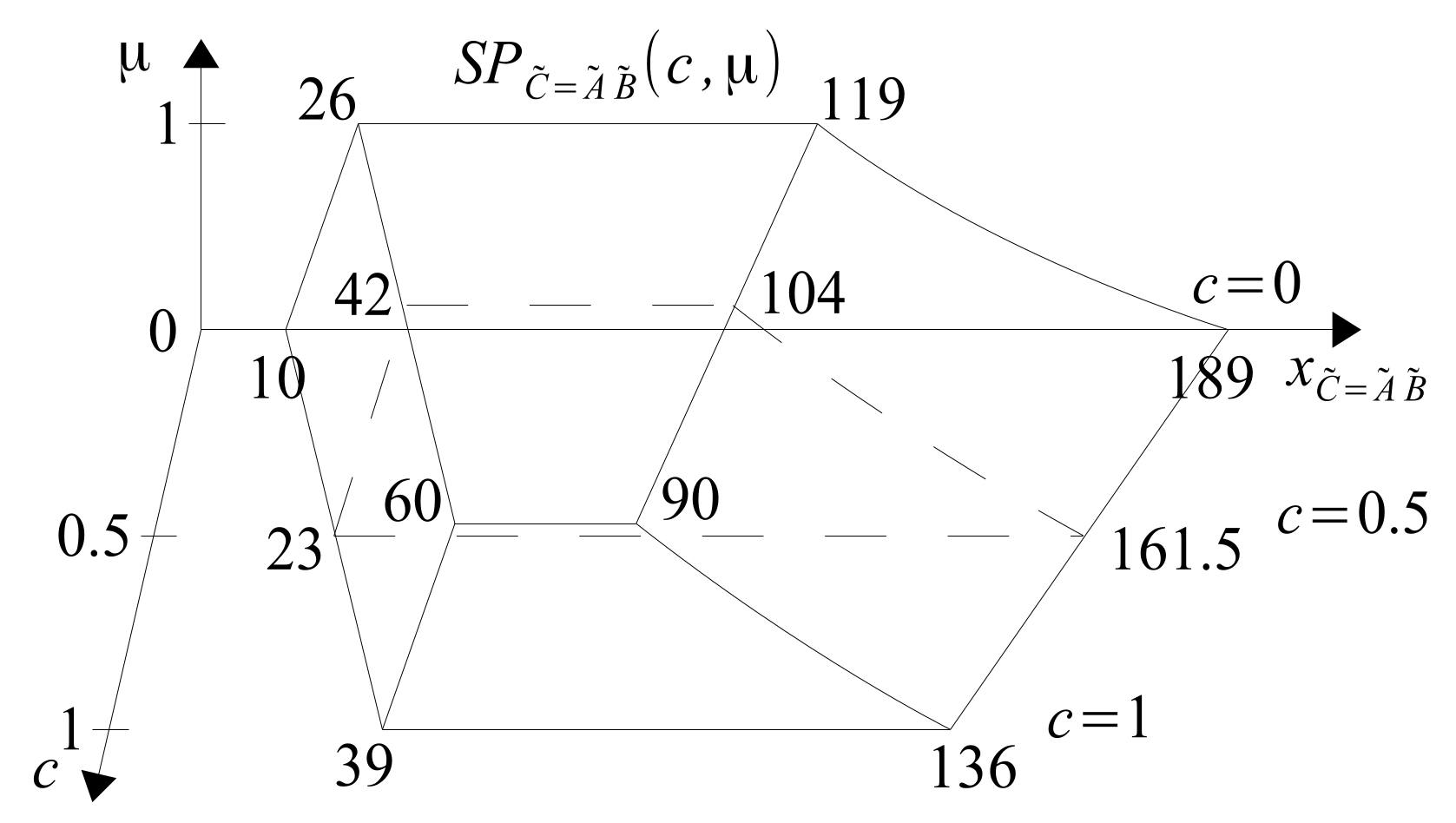
The span $S{P}_{\tilde{C}=\tilde{A}\tilde{B}}(c,\mu )$ of the resulting set $\tilde{C}$ of the multiplication $\tilde{A}\tilde{B}$ is shown in Figure 26 in 3D space, and Figure 27 shows $FOUS{P}_{\tilde{C}=\tilde{A}\tilde{B}}(c,\mu )$ in 2D space.

Both in Figure 26 and Figure 27, it can be seen that the left and right borders of the span function are smooth, monotonically increasing or decreasing. As will be shown later, this is not always the case with multiplication.

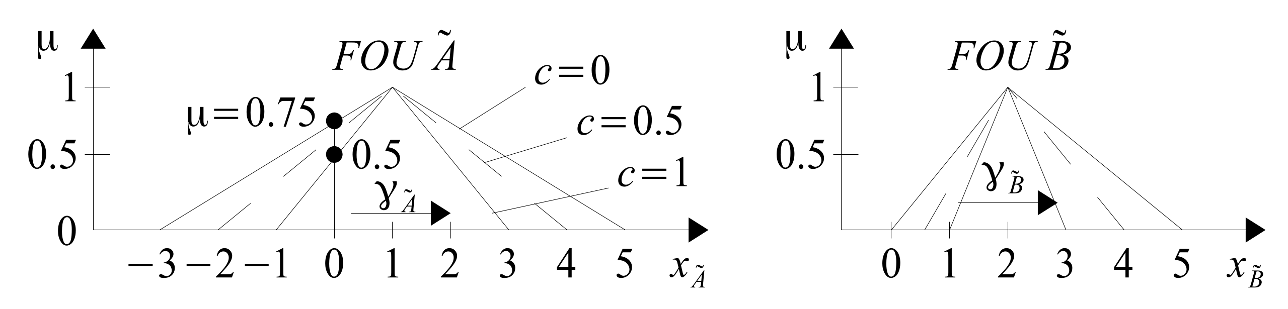
Multiplication of T2FNs containing zero

The multiplication of T2FNs containing zero is a bit more difficult than T2FNs without zero, because when the variable crosses zero, sign changes as a result of multiplication. On the lateral surfaces of the span function $S{P}_{\tilde{C}=\tilde{A}\tilde{B}}(c,\mu )$, inflection arises: these surfaces are no longer smooth. This phenomenon will be illustrated by the multiplication of triangular T2FNs $\tilde{A}$ and $\tilde{B}$, of which $\tilde{A}$ contains zero. $FOU\tilde{A}(x_{\tilde{A}},\mu )$ and $FOU\tilde{B}(x_{\tilde{B}},\mu )$ are shown in Figure 28.

We perform the multiplication operation according to general Formula (49).

$$\tilde{A}(c,{\gamma }_{\tilde{A}},\mu )\tilde{B}(c,{\gamma }_{\tilde{B}},\mu )=\tilde{C}(c,{\gamma }_{\tilde{A}},{\gamma }_{\tilde{B}},\mu ):x_{\tilde{A}}(c,{\gamma }_{\tilde{A}},\mu )x_{\tilde{B}}(c,{\gamma }_{\tilde{B}},\mu )=x_{\tilde{C}}(c,{\gamma }_{\tilde{A}},{\gamma }_{\tilde{B}},\mu ),c,{\gamma }_{\tilde{A}},{\gamma }_{\tilde{B}},\mu \in [0,1]$$

(49)

The number $\tilde{A}$ is given by the Formula (50) and the number $\tilde{B}$ by the Formula (51).

$$\tilde{A}(c,{\gamma }_{\tilde{A}},\mu ):x_{\tilde{A}}(c,{\gamma }_{\tilde{A}},\mu )=(-3+4\mu +2c-2c\mu )+{\gamma }_{\tilde{A}}(8-8\mu -4c+4c\mu ),c,{\gamma }_{\tilde{A}},\mu \in [0,1]$$

(50)

$$\tilde{B}(c,{\gamma }_{\tilde{B}},\mu ):x_{\tilde{B}}(c,{\gamma }_{\tilde{B}},\mu )=(2\mu +c+c\mu )+{\gamma }_{\tilde{B}}(5-5\mu -3c+3c\mu ),c,{\gamma }_{\tilde{B}},\mu \in [0,1]$$

(51)

By inserting the Formulas (50) and (51) into (49), we obtain the Formula (52) of the multivariate result of multiplication $\tilde{C}(c,{\gamma }_{\tilde{A}},{\gamma }_{\tilde{B}},\mu )$.

$$\begin{array}{c}\tilde{C}(c,{\gamma }_{\tilde{A}},{\gamma }_{\tilde{B}},\mu ):x_{\tilde{C}}(c,{\gamma }_{\tilde{A}},{\gamma }_{\tilde{B}},\mu )\hfill \\ =[(-3+4\mu +2c-2c\mu )+{\gamma }_{\tilde{A}}(8-8\mu -4c+4c\mu )][(2\mu +c+c\mu )+{\gamma }_{\tilde{B}}(5-5\mu -3c+3c\mu )],c,{\gamma }_{\tilde{A}},{\gamma }_{\tilde{B}},\mu \in [0,1]\hfill \end{array}$$

(52)

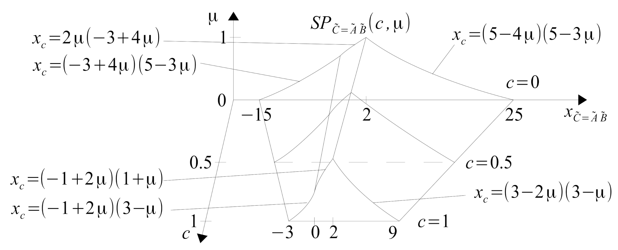
The multidimensional result (52) is the full, algebraic result of the multiplication and only it can be used for possible further calculations, e.g., in complex formulas. We cannot see this result. However, we can see the span function of this result, i.e., $S{P}_{\tilde{C}=\tilde{A}\tilde{B}}(c,\mu )$ (53). Since the number $\tilde{A}$ involved in the multiplication contains zero, a line of inflection will appear in $S{P}_{\tilde{C}=\tilde{A}\tilde{B}}$ in the point $x_{\tilde{C}}=x_{\tilde{A}}{x}_{\tilde{B}}=0$. The line of inflection of the function is visible on the surface of the function span, on the left, Figure 29 and Figure 30. The general way of determining the span for the multiplication result is given by the Formula (53), where $x_{\tilde{C}}(c,{\gamma }_{\tilde{A}},{\gamma }_{\tilde{B}},\mu )$ is given by the Formula (52).

$$S{P}_{\tilde{C}=\tilde{A}\tilde{B}}(c,\mu )=[\underset{{\gamma }_{\tilde{A}},{\gamma }_{\tilde{B}}}{min}{x}_{\tilde{C}}(c,{\gamma }_{\tilde{A}},{\gamma }_{\tilde{B}},\mu ),\underset{{\gamma }_{\tilde{A}},{\gamma }_{\tilde{B}}}{max}{x}_{\tilde{C}}(c,{\gamma }_{\tilde{A}},{\gamma }_{\tilde{B}},\mu )],c,{\gamma }_{\tilde{A}},{\gamma }_{\tilde{B}},\mu \in [0,1]$$

(53)

The examination of the Formula (54) shows that, for the range $x_{\tilde{A}}<0$ and $x_{\tilde{C}}<0$, the values of ${\gamma }_{\tilde{A}}$ and ${\gamma }_{\tilde{B}}$ determining $min{x}_{\tilde{C}}(c,{\gamma }_{\tilde{A}},{\gamma }_{\tilde{B}},\mu )$ are the values of ${\gamma }_{\tilde{A}}=0$ and ${\gamma }_{\tilde{B}}=1$. Whereas $max{x}_{\tilde{C}}(c,{\gamma }_{\tilde{A}},{\gamma }_{\tilde{B}},\mu )$ occurs for ${\gamma }_{\tilde{A}}={\gamma }_{\tilde{B}}=1$. For the range of values $x_{\tilde{A}}\ge 0$ and $x_{\tilde{C}}\ge 0$ $min{x}_{\tilde{C}}(c,{\gamma }_{\tilde{A}},{\gamma }_{\tilde{B}},\mu )$ occurs for ${\gamma }_{\tilde{A}}={\gamma }_{\tilde{B}}=0$ and $max{x}_{\tilde{C}}(c,{\gamma }_{\tilde{A}},{\gamma }_{\tilde{B}},\mu )$ holds for ${\gamma }_{\tilde{A}}={\gamma }_{\tilde{B}}=1$. Hence, ultimately the span of the multiplication result is given by Formula (54).

$$\begin{array}{c}\mathrm{For}{x}_{\tilde{A}}(c,{\gamma }_{\tilde{A}},\mu )<0\hfill \\ S{P}_{\tilde{C}=\tilde{A}\tilde{B}}(c,\mu )=[(-3+4\mu +2c-2c\mu )(5-3\mu -2c+4c\mu ),(5-4\mu -2c+2\mu c)(5-3\mu -2c+4c\mu )]\hfill \\ \mathrm{For}{x}_{\tilde{A}}(c,{\gamma }_{\tilde{A}},\mu )\ge 0\hfill \\ S{P}_{\tilde{C}=\tilde{A}\tilde{B}}(c,\mu )=[(-3+4\mu +2c-2c\mu )(2\mu +c+c\mu ),(5-4\mu -2c+2\mu c)(5-3\mu -2c+4c\mu )]\hfill \end{array}$$

(54)

When multiplying the numbers $\tilde{A}\tilde{B}$ for $x_{\tilde{A}}<0$, the negative part of the number $\tilde{A}$ is multiplied by the positive number $\tilde{B}$. For $x_{\tilde{A}}\ge 0$, the positive part of the number $\tilde{A}$ is multiplied by the positive number $\tilde{B}$. The span of the result of multiplication of the numbers $\tilde{A}\tilde{B}$ in 3D space is shown in Figure 29 and in 2D space in Figure 30. The presented example of the multiplication of numbers $\tilde{A}$ and $\tilde{B}$, one of which contains zero, showed that the presence of zero causes irregularity, deflection of the borders of span function.

The mathematical properties of type 2 fuzzy arithmetic are the same as the multidimensional T1FA properties mentioned in Section 2 and [41].

5. Application of T2FNs to Determine the Appropriate Dose of Nitrogen Fertilizer in the Cultivation of Sugar Beet

Real world problems are often complex, in the sense that the result variable y of interest to us depends on many and sometimes very many variables ($x_1,x_2,\dots ,x_n$) which we present in the form of the functional dependence $y=f(x_1,x_2,\dots ,x_n)$. In real problems, we often have no knowledge of the values of some variables that B.H. Yakov [47] called information gaps (Info-Gaps). Next, we have only approximate knowledge about another part of the variables and exact knowledge we have about only some variables. The prediction of the value of the dependent variable y then takes place under the conditions of uncertainty, additionally increased by the fact that our knowledge about the mathematical form of the relationship $y=f(x_1,x_2,\dots ,x_n)$ is also usually only approximate. Therefore, we cannot demand great precision from solutions to uncertain problems. Nevertheless, we should try to solve them as best as possible, using all available knowledge. An example of a highly uncertain problem is the cultivation of crops, such as sugar beets ($SB$). They provide a valuable break crop returning organic matter to the soil and preventing plant diseases. The beat-root cultivation starts at yield $[350,400]\left[\mathrm{q}/\mathrm{ha}\right]$. However, using appropriate agrarian methods, some of the growers receive yield $[600,800]\left[\mathrm{q}/\mathrm{ha}\right]$. To achieve such high yield, the skill of $SB$ cultivation is not all that is needed. A grower also needs to be a little lucky, because the crops depend not only on the grower and his actions, but also on factors independent of humans, such as the degree of sunlight over the field in a given year (too small, small, average, high), on the temperatures (cold, warm, heat), the intensity of rainfall (no-drought, medium, too large-flooding of fields), the occurrence of plant diseases, pest infestation, etc. So, it is not only the grower’s activity itself that determines the yield. However, the proper agrotechnical culture is what can influence the increase of yields. Adequate soil fertility is one of the requirements for profitable $SB$ production. Nitrogen (N) is the most yield-influencing nutrient, and N-management is critical to obtain high $SB$-yield and quality. Phosphorus (P) is the next most influential nutrient, while levels of potassium (K), sulfur (S), and micronutrients usually are adequate for $SB$ production in most soils [48]. The value of soil tests for the prediction of nutrient availability in a given area depends on how well the sample collected represents the sampled area. We should remember that the collected samples relate only to a small area and do not exactly model the whole field. The effect of nitrogen fertilization in the field has been studied for many years and is well known in terms of its quality. 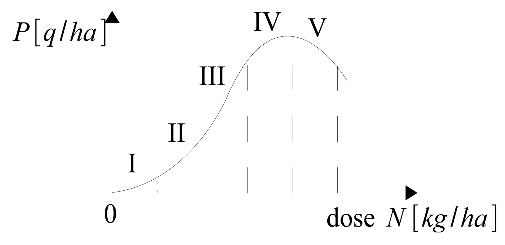This influence is mainly determined by Mitscherlich’s law of fertilization, Shelford’s maximum law and Shelford’s law of tolerance [49]. The typical dependence of the yield size $P\left[\mathrm{q}/\mathrm{ha}\right]$ on the nitrogen fertilizer dose $N\left[\mathrm{kg}/\mathrm{ha}\right]$ has the shape shown in Figure 31.

For each field, depending on the quality of its soil, sunlight, rainfall, temperatures, etc., this relationship is more or less quantitatively different, but qualitatively similar. The curve in Figure 31 has several specific ranges. Scope I concerns a very rare situation where $SB$ is grown on a poor quality soil and the fertilization dose is very low. Scope III is the range which is usually most frequent in the fertilizing trials. The range IV is the range of the excessive amount of the nutrient which causes mineral imbalance in the soil. Looking at this curve it is easy to understand how a major role plays appropriate amount of N for achieving high yield. However, it should be remembered that the grower operates under uncertainty and the fertilization curve for one and the same field changes gradually every year. Mathematically, the nitrogen fertilization curve can be approximated by the 2nd-order Equation (55). It is assumed that the range I, as it is very rare, does not apply to the field under consideration.

$$p=a_2{d}^2+a_{1}d+a_0=(a_{2}d+a_1)d+a_0$$

(55)

In the Equation (55), p denotes the $SB$ yield [q/ha] and d denotes the N-fertilizer dose $\left[\mathrm{kg}/\mathrm{ha}\right]$. The coefficients $a_0$, $a_1$, $a_2$ have their practical sense. The $a_0\left[\mathrm{q}/\mathrm{ha}\right]$ coefficient means yield from 1 ha with complete lack of fertilization. The $a_1$ factor represents (approximately) the increment of the yield due to the fertilization increase from $d=0$ to $d=1\left[\mathrm{kg}/\mathrm{ha}\right]$. The coefficient $a_2$ can be called the “braking” coefficient. It is negative and it represents a reduction in the impact of each next kilogram of fertilizer due to soil saturation. Note that, in order to identify very, very roughly the values of all 3 coefficients $a_0$, $a_1$, $a_2$, it is necessary to perform at least a 3-year field fertilization experiment, and still only average values of these coefficients for this 3-year period will be obtained. In the following years, slightly different values of these coefficients will be obtained due to the variability of environmental influences. The research on the values of the coefficients is tedious and requires many years. Usually, for the field of interest to us, we have a small number of measurements. Let us now assume that, on the basis of the conducted experiments for a certain field, it was found that the coefficient $a_0$ of zero-fertilization ranges from $[250,450]$, but usually it is within the range $[300,350]$. The yield increment coefficient $a_1$ is generally within the range $[3.0,3.6]$, but usually within the range $[3.0,3.3]$. The inhibition factor $a_2$ is generally in the range $[-0.012,-0.010]$, but most of its values are in the range $[-0.011,-0.010]$.

There are global ranges of the values of the coefficients and the ranges of the highest reliability of these coefficients.

Knowledge of the fertilization rates can be represented in the form of T2FNs shown in Figure 32, Figure 33 and Figure 34.

Knowledge about the values of the fertilization rates does not necessarily have to be provided in the form of 3D drawings. We can more easily present it in the form of FOUs of ${\tilde{A}}_0$, ${\tilde{A}}_1$, ${\tilde{A}}_2$ in 2D space, as shown in Figure 35.

The formula for the optimal dose value of N-fertilizer $d_{opt}$ can be derived on the basis of the 1st derivative of the yield p from Formula (55). If the fertilization rates are known exactly, the result is given by Formula (56).

$$d_{opt}=-\frac{a_1}{2a_2}$$

(56)

The optimal $d_{opt}$ fertilization value corresponds to the maximum $SB$-yield $p_{max}$, Formula (57).

$$p_{max}=a_0-\frac{a_1^2}{4a_2}$$

(57)

It should be remembered that the values of the $a_2$ coefficient are negative. Therefore, there must be a dependency $p_{max}\ge a_0$ which means that each fertilization increases the SB-yield. Since our knowledge of the values of $a_0$, $a_1$, $a_2$ is only approximate, we need to develop mathematical models of T2FNs ${\tilde{A}}_0$, ${\tilde{A}}_1$, ${\tilde{A}}_2$ and then calculate the multivariate result (recommended fertilization) $D_{opt}$ and the corresponding yield $P_{max}$. To do this, perform the calculations presented in Formula (58).

$$D_{opt}=-\frac{{\tilde{A}}_1}{2{\tilde{A}}_2},P_{max}={\tilde{A}}_0-\frac{{\tilde{A}}_1^2}{4{\tilde{A}}_2}$$

(58)

Based on the knowledge of $a_0$, $a_1$, $a_2$ contained in Figure 32, Figure 33 and Figure 34, mathematical formulas of T2FNs representing this knowledge were developed, (59)–(61).

$${\tilde{A}}_0(c,\mu ,{\gamma }_0):a_0(c,\mu ,{\gamma }_0)=(250+50\mu -50c\mu )+{\gamma }_0(200-150\mu -150c+150c\mu ),c,\mu ,{\gamma }_0\in [0,1]$$

(59)

$${\tilde{A}}_1(c,\mu ,{\gamma }_1):a_1(c,\mu ,{\gamma }_1)=3+{\gamma }_1(0.6-0.3\mu -0.3c+0.3c\mu ),c,\mu ,{\gamma }_1\in [0,1]$$

(60)

$$\begin{array}{c}{\tilde{A}}_2(c,\mu ,{\gamma }_2):a_2(c,\mu ,{\gamma }_2)=(-0.012+0.001\mu +0.001c-0.001c\mu )+{\gamma }_2(0.002-0.001\mu -0.001c+0.001c\mu ),\\ c,\mu ,{\gamma }_2\in [0,1]\end{array}$$

(61)

Based on the Formulas (56) and (58), it is possible to determine the set $D_{opt}$ of all possible values of the optimal fertilization dose $d_{opt}$, Formula (62).

$$\begin{array}{c}{D}_{opt}(\mu ,c,{\gamma }_1,{\gamma }_2)=-\frac{{\tilde{A}}_1(\mu ,c,{\gamma }_1)}{2{\tilde{A}}_2(\mu ,c,{\gamma }_2)}:\hfill \\ d_{opt}(\mu ,c,{\gamma }_1,{\gamma }_2)=\frac{1.5+{\gamma }_1(0.3-0.15\mu -0.15c+0.15c\mu )}{(0.012-0.001\mu -0.001c+0.001c\mu )+{\gamma }_2(-0.002+0.001\mu +0.001c-0.001c\mu )},c,\mu ,{\gamma }_1,{\gamma }_2\in [0,1]\hfill \end{array}$$

(62)

What does the fact that the set $D_{opt}(\mu ,c,{\gamma }_1,{\gamma }_2)$ is 5D mean and how can we understand it? Knowledge about the optimization of the $d_{opt}$ fertilizer dose has made it possible to determine the set $D_{opt}$ containing all possible $d_{opt}$-values corresponding to different degrees of membership $\mu$, various degrees of confidence c in possible T1MFs, and located at different relative distances ${\gamma }_1$, ${\gamma }_2$ from the membership function borders. The values of $\mu$, c, ${\gamma }_1$, ${\gamma }_2$ can be defined as features or attributes of individual possible values of $d_{opt}$. For example, the values of $\mu =0$, $c=0$, ${\gamma }_1=0.2$, ${\gamma }_2=0.3$ correspond to the value of the $d_{opt}=137.423\left[\mathrm{kg}/\mathrm{ha}\right]$ and the values of $\mu =0.9$, $c=0.8$, ${\gamma }_1=0.7$, ${\gamma }_2=0.6$ correspond to the value of the $d_{opt}=171.359\left[\mathrm{kg}/\mathrm{ha}\right]$. The number of possible quintuples $(\mu ,c,{\gamma }_1,{\gamma }_2)$ that can occur is infinite. Since the set $D_{opt}(\mu ,c,{\gamma }_1,{\gamma }_2)$ exists in 5D space, it cannot be seen. However, you can determine and view its span $S{P}_{Dopt}(\mu ,c)$ calculated from Formula (63).

$$S{P}_{Dopt}(\mu ,c)=[\underset{{\gamma }_1,{\gamma }_2}{min}{d}_{opt}(\mu ,c,{\gamma }_1,{\gamma }_2),\underset{{\gamma }_1,{\gamma }_2}{max}{d}_{opt}(\mu ,c,{\gamma }_1,{\gamma }_2)],\mu ,c,{\gamma }_1,{\gamma }_2\in [0,1]$$

(63)

Examination of the dependencies (62) and (63) allows one to establish that $min{d}_{opt}(\mu ,c,{\gamma }_1,$${\gamma }_2)$ holds for ${\gamma }_1={\gamma }_2=0$, and that $max{d}_{opt}(\mu ,c,{\gamma }_1,{\gamma }_2)$ for ${\gamma }_1={\gamma }_2=1$. Finally, we get the result (64).

$$\begin{array}{c}S{P}_{Dopt}(\mu ,c)=\left[\frac{1.5}{0.012-0.001\mu -0.001c+0.001c\mu },\frac{1.8-0.15\mu -0.15c+0.15c\mu }{0.001}\right],\mu ,c\in [0,1]\end{array}$$

(64)

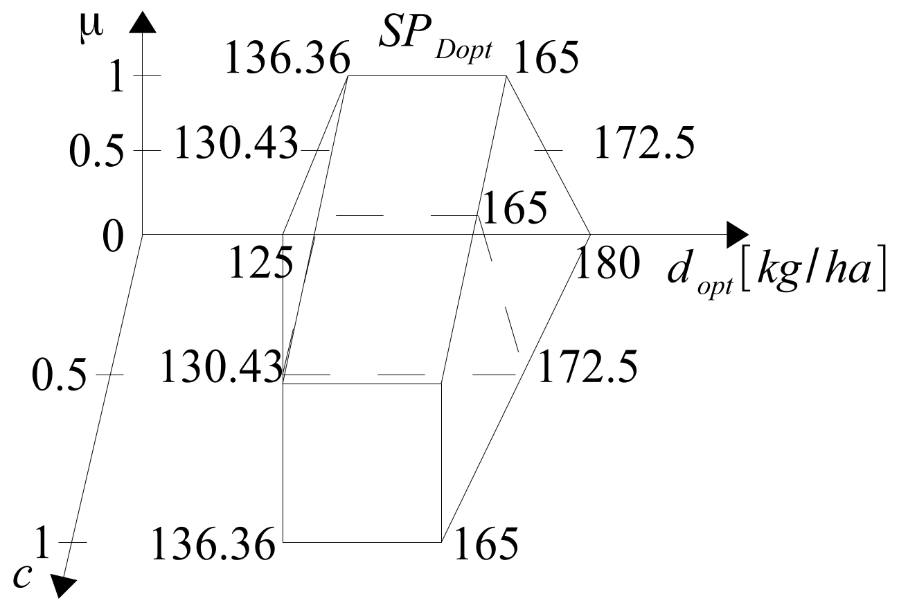
The 3D visualization of the span $S{P}_{Dopt}(\mu ,c)$ is presented in Figure 36.

Based on the uncertain knowledge contained in the span $S{P}_{Dopt}(\mu ,c)$, the plantation owner has to make a decision on the choice of a specific dose d of fertilizer. This dose can be determined by the defuzzification of the span function $S{P}_{Dopt}(\mu ,c)$. 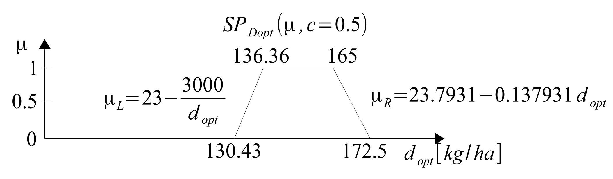Defuzzification means determining a single numerical $d_{opt}$-value that represents the entire $S{P}_{Dopt}(\mu ,c)$ set of possible $d_{opt}$ values, as well as possible or even optimally. A sensible method may be 2-step defuzzification. In step 1, the average T1MF is determined from the set of all possible T1MFs, each of which is one of the cuts of $S{P}_{Dopt}(\mu ,c)$ made for the selected value of confidence degree c. The average T1MF ${}_{aver}$ is the T1MF ($\mu ,c=0.5$) shown in Figure 37.

In the second step of defuzzification of the span function $S{P}_{Dopt}(\mu ,c)$, the average function $S{P}_{Dopt}(\mu ,c=0.5)$ should be defuzzified with e.g., the center of gravity method, according to Formula (65).

$$d_{opt}^{*}=\frac{\underset{130.43}{\overset{172.5}{\int }}{d}_{opt}·\mu \left(d_{opt}\right)·d\left(d_{opt}\right)}{\underset{130.43}{\overset{172.5}{\int }}\mu \left(d_{opt}\right)·d\left(d_{opt}\right)}\approx 151.1$$

(65)

As a result of defuzzification, the recommended dose $d_{opt}\approx 151.1$ of nitrogen fertilizer for the field in question is obtained, resulting from fertilization function (55).

In the next step of solving the problem, it is possible to determine the expected value of the yield $P_{max}$ determined by the Equations (57) and (58). Figure 38 shows the span function $S{P}_{Pmax}(\mu ,c)$.

Figure 39 shows the FOU $S{P}_{Pmax}\left(\mu \right)$.

The span functions of possible $SB$-yields on the field under consideration obviously do not give a precise answer as to how big the yield will be, because it is impossible. Furthermore, no one can give such an accurate answer. However, the span functions show the possible ranges in which the future yield $P_{max}$ may be located. The accuracy of these ranges results from the knowledge of the field and the knowledge of fertilization dependencies in $SB$ cultivation.

6. Conclusions

The article characterizes the current state of fuzzy arithmetic type 1 and type 2 based on the border definitions of fuzzy sets type 1 and type 2. Next, a new “body” definition of T2FS was presented, which in the authors’ opinion, is more suitable for arithmetic calculations than the current border definition. The paper recalls type 1 multivariate arithmetic, which is the basis of T2FA, paying special attention to the explanation and justification of the multidimensionality of this arithmetic. It also covers the basic arithmetic operations of T2FA and shows some simple calculation examples. To show the application of multidimensional T2FN, a more complex example of the use of T2FA in the problem of sugar beet fertilization is presented—a problem with a high share of uncertainty. This article presents T2FA for normal FNs, which, according to the authors’ opinion, introduces some progress in this arithmetic. However, it is not the end of the work. The further development of T2FA is needed. As a next step in this development, T2FA should be developed for non-normal T2FNs. An example of FOU of normal and non-normal T2FN is given in Figure 40.

Knowledge of how to perform calculations on normal T2FNs will greatly facilitate the development of T2FA for non-normal T2FNs. Non-normal T2FNs may arise (as representation of expert knowledge) when there are strong differences in a group of many experts in the estimation of uncertain values of variables.