Structural Health Monitoring Using Machine Learning and Cumulative Absolute Velocity Features

Abstract

Machine learning (ML)-aided structural health monitoring (SHM) can rapidly evaluate the safety and integrity of the aging infrastructure following an earthquake. The conventional damage features used in ML-based SHM methodologies face the curse of dimensionality. This paper introduces low dimensional, namely, cumulative absolute velocity (CAV)-based features, to enable the use of ML for rapid damage assessment. A computer experiment is performed to identify the appropriate features and the ML algorithm using data from a simulated single-degree-of-freedom system. A comparative analysis of five ML models (logistic regression (LR), ordinal logistic regression (OLR), artificial neural networks with 10 and 100 neurons (ANN₁₀ and ANN₁₀₀), and support vector machines (SVM)) is performed. Two test sets were used where Set-1 originated from the same distribution as the training set and Set-2 came from a different distribution. The results showed that the combination of the $CAV$ and the relative $CAV$ with respect to the linear response, i.e., $R_{CAV}$, performed the best among the different feature combinations. Among the ML models, OLR showed good generalization capabilities when compared to SVM and ANN models. Subsequently, OLR is successfully applied to assess the damage of two numerical multi-degree of freedom (MDOF) models and an instrumented building with $CAV$ and $R_{CAV}$ as features. For the MDOF models, the damage state was identified with accuracy ranging from 84% to 97% and the damage location was identified with accuracy ranging from 93% to 97.5%. The features and the OLR models successfully captured the damage information for the instrumented structure as well. The proposed methodology is capable of ensuring rapid decision-making and improving community resiliency.

1. Introduction

The past decade has seen unprecedented levels of innovation in data science with major advancements in computing and sensing technologies. These growing resources in the field of artificial intelligence (AI), particularly in machine learning (ML), have opened up new possibilities for structural health monitoring (SHM). AI aided SHM can become a viable way of addressing the challenges faced by the dwindling US infrastructure systems, which received a grade of “C−” by the American Society of Civil Engineers’s (ASCE) national infrastructure report card in 2021 [1]. In fact, the same report card cited that “living structures” where sensors are being embedded into new and existing structures to provide continuous feedback on the structural conditions, is a promising innovation to look forward towards the next generation built environment.

Advances in remote sensing, computing technologies, and ML in the past few years paved the way to enable the idea of “living structures”. ML assists computers to learn about the trends and features of a process without being explicitly programmed. In SHM, the learning problem is to find the relationship between damage and measured (training) data [2]. Conventional ML tools were, however, limited in their ability to process the large amounts of measured sensor data in their raw form, particularly before deep learning (DL) tools emerged. As such, careful engineering and considerable domain knowledge have been utilized to extract damage-sensitive features from the raw data which were subsequently fed into a suitable ML model. Many of these features were based on modal properties of the structure, such as modal frequencies, mode shapes, curvature of mode shapes, modal assurance criteria, and power spectral densities [3,4,5,6,7,8]. Although these damage-sensitive features produced promising results [9,10], they were also shown to be sensitive to operational or environmental conditions [11]. Therefore, researchers have studied alternative features not based on modal properties, such as the cumulative absolute velocity ($CAV$) [12,13], higher exponentiations of the acceleration intensity [14], standardized $CAV$ ($CA{V}_{STD}$) [15], and instantaneous power ($IP$) [16], which also showed promising results for SHM [17].

Applications of ML in vibration based-SHM have been studied by several researchers [18,19,20]. Among different ML models, multi-layer perceptrons (MLP) have been applied the most [21,22,23,24]. Lam et al. [18] proposed a Bayesian artificial neural network (ANN) method for SHM and showed its applicability for a truss bridge. Pawar et al. [25] used Fourier coefficients of the mode shapes with ANN to detect and locate damage. Mehrooj et al. [26] used an ANN based system identification method to estimate damage percentage of joints for a truss bridge structure. More recently, developments of convolutions neural network (CNN) based SHM techniques are increasing. Abdeljaber et al. [27] trained CNN models for different damage cases and successfully classified damage. Khodabandehlou et al. [28] applied two dimensional (2D) CNN for the overall assessment of concrete bridges. Support vector machine (SVM) is another ML classifier that researchers found effective in damage detection. Gui et al. [29] showed that optimized SVMs can detect and locate damage accurately with autoregressive (AR) coefficients and residual errors as features. Ghiasi et al. [30] used wavelet packet transform with least square SVM to detect damage. Pan et al. [31] demonstrated successful use of SVM models with wavelet transform, Hilbert-Huang transform (HHT), and Teager-Huang transform (THT) on a numerical cable stayed bridge model. In most of these studies, ambient vibrations were used as the input excitation. Earthquake vibrations caused by strong ground motion have rarely been utilized with ML classifiers. Moreover, most of the current ML aided SHM methodologies require high-dimensional features. As a result, the issue of the curse of dimensionality arises, i.e., the size of the training dataset needs to be large for such methodologies. This is a challenge for the earthquake damage assessment problem as the data from recorded earthquakes are usually limited in size. Low dimensional features are crucial for successful implementation of ML algorithms for such a problem. Besides, low-dimensional and computationally efficient models allow using ML for edge devices and enable real-time damage assessment. Therefore, the study presented in this paper proposes a novel approach that uses low-dimensional damage features in ML classification models on strong motion data of instrumented structures. Figure 1 shows the overview of the approach where CAV based features are extracted from the acceleration response of a structure following an earthquake. Subsequently, ML models are developed to detect and assess the condition of the structure.

2. Setting of the Computer Experiments

In this study, a computer experiment has been conducted to evaluate the damage detection and assessment capabilities of one-dimensional CAV based features. These features were extracted from acceleration responses of a single-degree-of-freedom (SDOF) system. Nonlinear time history analysis (NLTH) was utilized to generate the acceleration responses from this SDOF system. The computed features were subsequently utilized as training and test data for a comparative study between five well-known ML algorithms. In the following subsections, the computer experiment is described in detail.

2.1. Data Source

Data for this computer experiment came from the acceleration responses of a SDOF system. Section 2.1.1 describes the modeling details of the SDOF system. NTHA was utilized as the analysis method to generate the acceleration responses with two sets of ground motions as inputs. Section 2.1.2 describes these two sets of ground motions. For the damage detection and assessment tasks, it is important to clearly define the damage states as described in Section 2.1.3.

2.1.1. Analytical Model

The SDOF model used in this study was developed in OpenSees [32] using Steel01 material which has a bilinear behavior with strain hardening of 1%. The mass, stiffness, and damping of the SDOF system were based on pushover and eigenvalue analyses reported in [33,34]. The base shear coefficient ($\eta$), i.e., the ratio between the base shear at yield ($V{y}_{base}$) and the weight of the building (W), was taken as 0.2, as recommended by [35] for regular structures designed for seismic risk category D.

2.1.2. Ground Motion

Two different sets of data have been used in this study. Set-1 included responses of ground motions from the PEER NGA-West2 [36,37] database. This database has 21,539 records of shallow crustal earthquakes in active tectonic regions. Due to the possibility of anomalies from older data collection systems, only records from the past 30 years were selected. Moreover, records with peak ground acceleration (PGA) less than 1% of the acceleration of gravity (g) may not produce sufficient excitation useful for this study. Therefore, only records with PGA of more than 1%g were considered. Lastly, to avoid homogeneity in the response, not more than 20 records from a single event were selected. A total of 1710 records matched these criteria. Figure 2 shows the magnitude and hypocenter distance ranges of these selected records. The magnitude of these records varied from 3 to 8 with the majority (565) of records having a magnitude between 5 and 6 and about 200 records coming from events with magnitudes of 7–8. On the other hand, 28% of these records (480) had a hypocenter distance less than 25 km and 15% of the records corresponded to a hypocenter distance greater than 100 km. This shows that the records covered near-field and far-field events with variability in magnitude.

Set-2 comprised responses to site-specific ground motions used in [38]. These ground motions were selected by matching the uniform hazard spectrum and associated causal events for a site in Oakland, California. It consisted of 120 ground motions representing three hazard levels, namely 2%, 10%, and 50% probabilities of exceedance in 50 years. Figure 3 shows that these records were mostly higher magnitude events (M > 6) and 98% of the records had hypocenter distance less than 50 km. With such a set, it was expected that the majority of these records would push the structure into the nonlinear range of the response to evaluate the ability of the proposed features for damage assessment.

2.1.3. Damage States

The maximum displacement ductility, $\mu$, is commonly used to quantify the structural damage.

$$\mu =max\left[\frac{d_{si}}{d_y}\right],$$

(1)

where $d_{si}$ is the maximum displacement experienced by the structure during the loading cycle i and $d_y$ is the yield displacement. If the structure sustains residual displacement, $d_r$, in cycle $i-1$, the displacement for cycle i is calculated as $d_{si}=d-d_r$, where d is the displacement relative to the original “undeformed” position. The displacement ductility index is based on the peak displacement to represent the damage caused by excessive deformations while neglecting the fatigue effect of cyclic loads. For an undamaged case, $\mu$ is smaller than 1.0 and the higher its value, the greater the expected damage. In this experiment, the damage states were divided into three categories according to FEMA P-58 [39]: $1\le \mu \le 2$ as minor damage, $2<\mu \le 6$ as moderate damage, and $\mu >6$ as major damage.

Figure 4 shows the percentage of records producing each damage state for Set-1 and Set-2. For Set-1, the structure remained undamaged for 1215 (71%) records while 308 (18%), 143 (8%), and 45 (3%) records caused minor, moderate, and major damages, respectively. This was representative of a database from real instrumented structures where most of the collected data are attributed to undamaged structures and very few data from severely damaged structures. On the contrary, for Set-2, 5%, 29%, and 66% records caused minor, moderate, and major damages, respectively.

2.2. Features

In this section, the one-dimensional CAV based features are described. The CAV has been used as an earthquake intensity measure [40] where it was shown that ground motion CAV has a better correlation to damage than other intensity measures, e.g., PGA, spectral acceleration, or effective duration. However, until recently, CAV of floor accelerations has not been used in SHM to assess damage. Muin and Mosalam [13] introduced CAV as a damage feature showing that CAV time series, its normalized version (NCAV), and other features extracted from it had distinct patterns for damaged structures which can be used to identify and locate damage. In this paper, four CAV based damage features, discussed below, were studied. These are one-dimensional features making them appropriate for ML computing environment with limited-size datasets.

2.2.1. Maximum CAV of Structural Response

The maximum CAV of the structural response, $CAV$, is defined as follows,

$$CAV\left(t\right)={\int }_0^T\left|\ddot{u}\left(t\right)\right|dt,$$

(2)

where $|\ddot{u}\left(t\right)|$ is the absolute value of acceleration at time t and T is the total duration of the recorded acceleration. For the $CAV$ calculation herein, the considered acceleration was the floor accelerations of a building. A higher $CAV$ value was expected in damaging events than in undamaged cases as damaging events are expected to be either correlated to high amplitude motion or to long duration.

2.2.2. Relative CAV

The relative CAV, $R_{CAV}$, is defined as follows,

$$R_{CAV}=\frac{CA{V}_s}{CA{V}_l},$$

(3)

where $CA{V}_s$ is the $CAV$ of the floor acceleration, and $CA{V}_l$ is the $CAV$ of the corresponding linear system excited by the same ground acceleration. For an undamaged case and accurate linear model, this value is 1.0. With damage, the acceleration amplitude typically decreases compared to the linear case due to the lengthening of the natural period, i.e., $R_{CAV}$ was expected to decrease with increasing damage states.

2.2.3. Difference in Effective Duration

The definition of the difference in effective duration, $S_{CAV}$, is as follows,

$$S_{CAV}=\frac{D_{5-75,s}-D_{5-75,l}}{D_{5-75,l}}\times 100\%.$$

(4)

The parameter $D_{5-75}$ above is the effective duration of an earthquake [41] defined by the time to achieve 75% of the $CAV$ value starting from the 5% of that value. It was expected that higher $S_{CAV}$ is associated with higher damage while for an undamaged case, this value is 0.0.

2.2.4. Total Deviation of CAV

The total deviation of CAV is calculated by taking the absolute difference of the area under the $CAV$ plots of an actual event and the corresponding linear state. The change of pattern in $CAV$ time series and its linear counterpart provides useful information about the damage. However, the comparison at each point of observation makes it a very high dimensional feature. Hence, the area is calculated as a compact (low dimension) feature.

$${\Delta }_{CAV}=\frac{|A_s-A_l|}{A_l}\times 100\%,$$

(5)

where $A_s$ and $A_l$ are the areas under the CAV plot of a structure and its corresponding linear system, respectively. This value was expected to increase with damage, while for an undamaged case, it is 0.0.

2.3. Exploratory Data Analysis

This section presents the exploratory data analysis conducted to identify suitable features. For this purpose, the relationships of each feature to different damage states were observed. A good feature demonstrates a certain pattern with increasing damage. Figure 5 shows the relationships of each of the four considered features with the displacement ductility for the entire dataset (Set-1 and Set-2). In these plots, the green, yellow, orange, and red circles represent undamaged, minor damage, moderate damage, and major damage cases, respectively.

The $CAV$ values showed an increasing trend with the increase of the displacement ductility. However, undamaged and minor damage $CAV$ values were difficult to distinguish. On the other hand, the $R_{CAV}$ distinguished undamaged from minor damage where $R_{CAV}$ values other than 1.0 correspond to damaged cases. Although for significant damage, the acceleration of the structure typically decreases, for certain ground motions where the undamaged structural responses fall on the initial ascending branch of the response spectrum, small damage leads to an increase in acceleration and subsequently an increase in the $R_{CAV}$ value. The overall decreasing pattern with increasing ductility of this feature made it well-suited for damage assessment. The ${\Delta }_{CAV}$ values showed a nonlinear increasing trend with the increase of the displacement ductility. Finally, the $S_{CAV}$ did not show any specific trend with displacement ductility, making it unsuitable as a damage feature.

2.4. ML Models

Five ML models were considered in the computer experiment, namely, logistic regression (LR), ordinal logistic regression (OLR), two artificial neural networks (ANN), and support vector machine (SVM). These models allow to calculate the probabilities of being in a damage category, making them suitable for structural damage assessment to provide information about the underlying uncertainty in SHM. Additionally, such models provide the decision maker with the opportunity to adopt probabilistic decision-making frameworks [42,43]. Details of each of these models are described below.

2.4.1. Logistic Regression

The LR is a technique applied to problems with binary response variable y, i.e., the number of available categories is two. The model conducts a linear mapping $\theta x$, on the $d+1$ dimensional input feature space of x considering a bias term, where $\theta \in {\mathbb{R}}^{d+1}$. Subsequently, through a sigmoid transformation (Equation (6)), the probability of a given data vector $x_i$ classified as 1 is calculated by Equation (7).

$$h\left(x\right)=\frac{1}{1+e^{-x}},$$

(6)

$$P(y_i=1|x_i)=h\left(\theta x_i\right),$$

(7)

where $\theta x_i$ is a linear combination of the features and 1 is the damage class (0 is for the undamaged class). For m samples, $\theta$ is determined by minimizing the loss function, as follows,

$$L\left(\theta \right)=\sum _{i=1}^m\left\{y_{i}ln\left[h\left(\theta x_i\right)\right]+(1-y_i)ln[1-h\left(\theta x_i\right)]\right\}.$$

(8)

When the number of categories is more than two, the LR can still be applied for classification using an approach called “one vs all” approach where one damage class is labeled as 1 and the others are labeled as 0 for training and the process is repeated for each class. Using Equation (7) and the training set, the coefficient vectors $\theta$ are evaluated. In this study, the four damage categories were assigned 0 (undamaged), 1 (minor damage), 2 (moderate damage), and 3 (major damage). The LR model finds the linear boundary that separates each damage category from the others.

2.4.2. Ordinal Logistic Regression

The OLR is used when the response variables represent ordered phenomenon and have multiple classes. For the problem considered in this study, the classes or damage categories were ordered and, hence, OLR was suitable. In OLR, the event of interest is a particular damage state and the lesser ones. The probability of the i-th input vector, $x_i$, classified as being in or lower than a damage state f is computed by Equation (9). Through the sigmoid transformation, Equation (6), the formulation is shown in Equation (10).

$$P(y_i\le f|x_i)=h\left(\theta x_i\right),$$

(9)

$$ln\left[\frac{P(y_i\le f|x_i)}{P(y_i>f|x_i)}\right]=\theta x_i.$$

(10)

The optimization problem for OLR is the same as that for LR (Equation (8)). The OLR model finds the linear boundary between a damage class and the higher damage classes, i.e., boundary 1 separates category 0 (coefficient vector ${\theta }_0$) from 1 to 3, boundary 2 separates categories 0 and 1 (coefficient vector ${\theta }_1$) from 2 and 3, and boundary 3 separates categories 0, 1, and 2 (coefficient vector ${\theta }_2$) from 3. Consequently, damage probabilities of the j-th sample of the test case are evaluated using the following equations,

$$P(y_j=0|x_j)=P(y_j\le 0|x_j)=h\left({\theta }_0{x}_j\right),$$

(11)

$$P(y_j=1|x_j)=P(y_j\le 1|x_j)-P(y_j=0|x_j)=h\left({\theta }_1{x}_j\right)-h\left({\theta }_0{x}_j\right),$$

(12)

$$P(y_j=2|x_j)=P(y_j\le 2|x_j)-P(y_j\le 1|x_j)=h\left({\theta }_2{x}_j\right)-h\left({\theta }_1{x}_j\right),$$

(13)

$$P(y_j=3|x_j)=1.0-P(y_j\le 2|x_j)=1.0-h\left({\theta }_2{x}_j\right).$$

(14)

2.4.3. Artificial Neural Network

The ANN is the most commonly used ML tool. It uses a large number of connected neurons and simulates the learning process of a biological brain. ANN architecture achieves powerful representation abilities and can approximate complex nonlinear functions. The network is comprised of three main layer types: input layer, hidden layer(s), and output layer. To obtain the best approximation, the large number of parameters in the neurons are trained with the input data through several iterations with the objective of minimizing the defined loss function. The workflow in the ANN consists of forward pass and backward propagation. In this study, the forward network architecture [44] was applied with the vector of damage features, x, as the input layer and two hidden layers with n neurons. The output variable y was stacked in a matrix after 1-hot encoding according to the four damage states. The input vector was multiplied by the weight vector w to obtain the output z of layer-1 as follows,

$$z=w^{T}x+b,$$

(15)

where b is a bias term and T represents transpose. Subsequently, z is used as the input to the activation function $\sigma (.)$ to produce the predicted outputs. In this study, the sigmoid function (Equation (6)) was used as the activation function. After the predicted outputs were computed, the total loss of the ANN can be computed based on the defined loss function $L(.)$ (Equation (8)). The results of two different ANN models were reported in this study, namely ANN₁₀ and ANN₁₀₀ with $n=10$ and 100 neurons, respectively.

2.4.4. Support Vector Machine

The SVM is a very common ML algorithm used for classification. SVM finds the optimum boundary separating the data of different classes to map the space of the original variables into an unknown high-dimensional feature space, where the data are linearly separable. This is performed by constructing a hyper-plane or a set of hyper-planes. The hyper-plane, H, is also known as the decision boundary and the data points closest to H are denoted as the support vector (SV) points. The distance between H and the SV points are known as the margin M. Equation (16) is the formulation of H where a is perpendicular to H and b is the offset of H from the origin along the normal vector a.

$$a^{T}x-b=0.$$

(16)

SVM is a binary classification algorithm which can be extended to handle multiclass problems. In this study, SVM applied the error correcting output code (ECOC) or the ”one-vs-one” approach for training. For the four classes specified in this study, six binary SVM models were used as learners. Minimizing the loss function was used as the decoding scheme where the loss function is represented as follows,

$$\underset{a,b}{min}\frac{1}{2}{\left|\right|a\left|\right|}^2\mathrm{s}.\mathrm{t}.y_i(a^T{x}_i-b)\ge 1,$$

(17)

where $\left|\right|a\left|\right|$ is the length of the vector a, i.e., its Euclidean norm.

3. Experimental Results

In this section, results of the computer experiment are presented. The experiment compared the ML algorithms LR, OLR, ANN₁₀, ANN₁₀₀, and SVM and it was performed using $CAV$, $R_{CAV}$, and ${\Delta }_{CAV}$ as features to determine the ideal features and ML algorithm. Two different training and test data sets were used where the first training set (TR-1) was a randomly sampled 85% of Set-1 data as the training set and the remaining 15% as the first test set (TE-1), i.e., both training and test were performed with data from the same distribution, which is the usual practice in ML. The second training set (TR-2) was the entire Set-1 while the second test set (TE-2) was Set-2, to test the robustness of the features using data from a different distribution than that of the training data.

As the performance parameter, the test accuracy was computed as follows,

$$\mathrm{Accuracy}=\frac{TP+TN}{TP+FP+TN+FN}\times 100\%,$$

(18)

where $TP$ is True Positive, $TN$ is True Negative, $FP$ is False Positive, and $FN$ is False Negative. In these definitions, Positive and Negative imply damaging and undamaged events, respectively.

Table 1. Accuracy (%) of ML models for different feature combinations (Set-1: training & test).

Input Feature	OLR	LR	ANN${}_{10}$	ANN${}_{100}$	SVM
$CAV$	80.54	82.88	80.54	81.71	79.38
$R_{CAV}$	87.16	86.72	88.72	89.49	88.33
${\Delta }_{CAV}$	75.10	75.10	75.10	77.04	75.10
$CAV,R_{CAV}$	90.27	89.44	88.72	90.66	91.05
$R_{CAV},{\Delta }_{CAV}$	86.77	84.72	89.11	87.94	87.94
$CAV,{\Delta }_{CAV}$	80.54	83.27	80.54	81.32	79.38
$CAV,R_{CAV},{\Delta }_{CAV}$	90.27	89.05	90.27	90.66	89.88

and

Table 2. Accuracy (%) of ML models for different feature combinations (Set-1: training & Set-2: test).

Input Feature	OLR	LR	ANN${}_{10}$	ANN${}_{100}$	SVM
$CAV$	36.67	12.50	18.33	15.83	8.33
$R_{CAV}$	60.00	42.50	30.83	37.50	20.83
${\Delta }_{CAV}$	61.67	45.00	42.50	40.00	21.67
$CAV,R_{CAV}$	74.14	61.67	18.33	40.00	25.00
$R_{CAV},{\Delta }_{CAV}$	65.83	45.00	60.00	40.00	22.50
$CAV,{\Delta }_{CAV}$	70.00	60.00	51.67	36.67	24.17
$CAV,R_{CAV},{\Delta }_{CAV}$	70.00	61.67	38.33	54.17	25.00

report the accuracy achieved by each model for TE-1 and TE-2, respectively. Table 1 shows that the highest accuracy of 91.05% was achieved by the SVM model with $CAV$ and $R_{CAV}$ as features. ANN₁₀₀ and OLR achieved accuracy values of 91% and 90%, respectively, with the same features. As expected, when the dataset was of a big size and the data were representative of the population (i.e., training and test sets came from the same target unknown distribution), the results were not significantly affected by the choice of the ML algorithm. On the other hand, when the ML algorithms were tested over a different set of data, their predictive capabilities were significantly reduced (Table 2). For this latter case, the accuracy reduced for each model, where OLR achieved the highest accuracy of 74.14% with $CAV$ and $R_{CAV}$ features. This was due to the fact that ANN and SVM over-fitted the data of the training set and had poor generalization capabilities over the response of different ground motions. Moreover, the simpler models of LR and OLR had better generalization capabilities.

From Table 2, one observes that the OLR was the most robust algorithm for making predictions about events not available in the training set. Moreover, in both test sets, satisfactory performances were obtained using $R_{CAV}$, while the best results were achieved using both $CAV$ and $R_{CAV}$ as features. For this reason, along with the fact that the computational demand of OLR was significantly lower than that of the ANN or SVM, the ML algorithm OLR with features $CAV$ and $R_{CAV}$ was concluded to be suitable for vibration based damage detection tasks of instrumented buildings.

4. Applications

In this section, results from two example case studies are presented. In the first example, two MDOF models were used. In the second example, an instrumented building was studied.

4.1. MDOF Systems

4.1.1. Model Description

Two MDOF models representing two five story buildings were used in this case study (Figure 6a). The models were developed using Steel01 material in OpenSees [32] with the force-displacement behavior shown in Figure 6c. The mass, stiffness, and damping of each story of the MDOF systems were based on pushover and eigenvalue analysis conducted in previous studies [33,34]. One of the MDOF systems, MDOF-US, had uniform shear capacity along the height of the building which is equal to the calculated base shear ($V{y}_{base}$) at yield. The other MDOF system, MDOF-NS, was designed to have non-uniform shear capacity distribution along the height of the building. The shear capacity of MDOF-NS varied as follows,

$$V{y}_n=\left[1-(1-\delta ){\left(\frac{h_n}{H}\right)}^{\lambda }\right]\times V{y}_{base},$$

(19)

where $V{y}_n$ is the yield shear at story n, $h_n$ is the height of the n-th story from the base of the building, $\delta$ is the ratio of the lateral stiffness at the top of the building to that at the base of the building [45], and H is the total building height. Equation (19) was proposed in [45] to take into account nonuniform stiffness of multistory buildings. The values of $\delta$ and exponent $\lambda$ were taken as 0.3 and 1.5, respectively.

According to ASCE 7 [46], the induced shear force at story z, $V_z$, is determined as follows,

$$V_z=\sum _{i=z}^n{C}_{vi}V{y}_{base},C_{vz}=\frac{w_z{h}_z^p}{{\sum }_{i=1}^n{w}_i{h}_i^p},$$

(20)

where $C_{vz}$ is the vertical distribution factor, $w_z$ is the portion of the total effective seismic weight at story z, $h_z$ is the height of the story z from the base of the building, and p is an exponent related to the building natural period, $T_n$. For $T_n<0.5$ s, $p=1.0$, for $T_n>2.5$ s, $p=2.0$, and for $0.5\le T_n\le 2.5$, p is linearly interpolated. Thus, for the MDOF system at hand, $p=1.075$.

Table 3. Story shear to base shear ratios.

Story	Code Minimum	MDOF-NS Design	MDOF-US Design
1	1.00	1.00	1.00
2	0.93	0.94	1.00
3	0.81	0.82	1.00
4	0.61	0.67	1.00
5	0.34	0.49	1.00

shows the story values of the shear to base shear ratios according to code [46] and for the two MDOF systems where the design of both systems was code conforming. However, MDOF-NS marginally met the code whereas MDOF-US had significantly higher values throughout the height and is a more conservative design which is often the case for low-to-medium rise buildings. For each model, a corresponding linear system was also developed using the Elastic material from OpenSees [32].

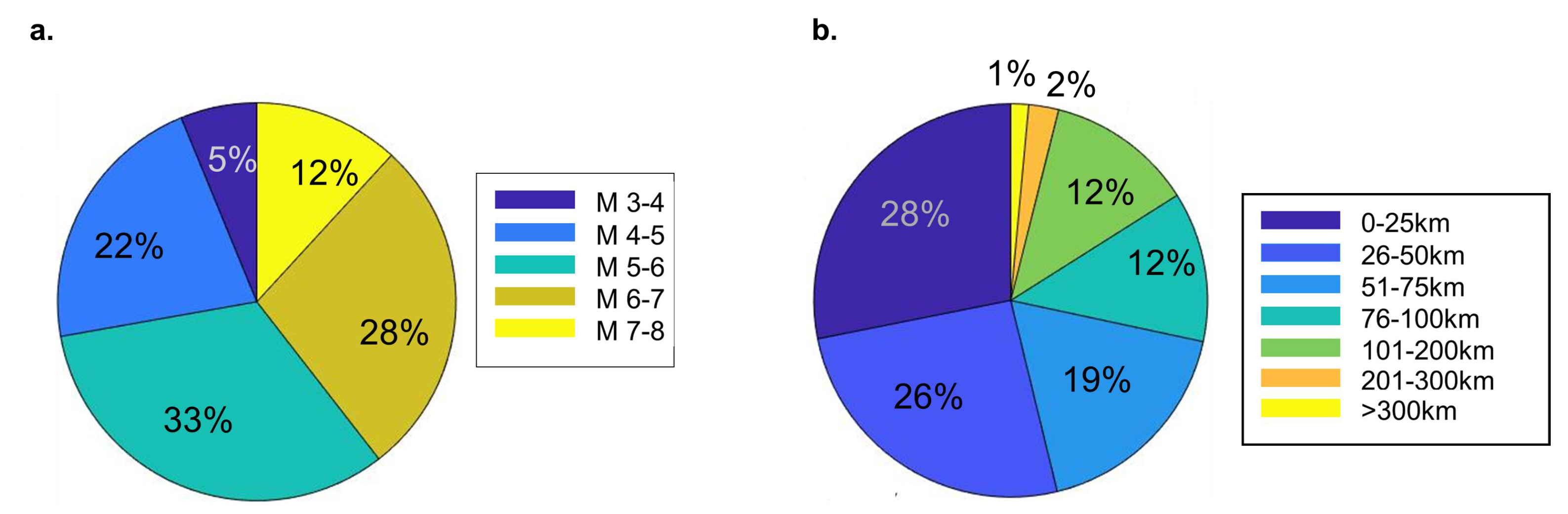
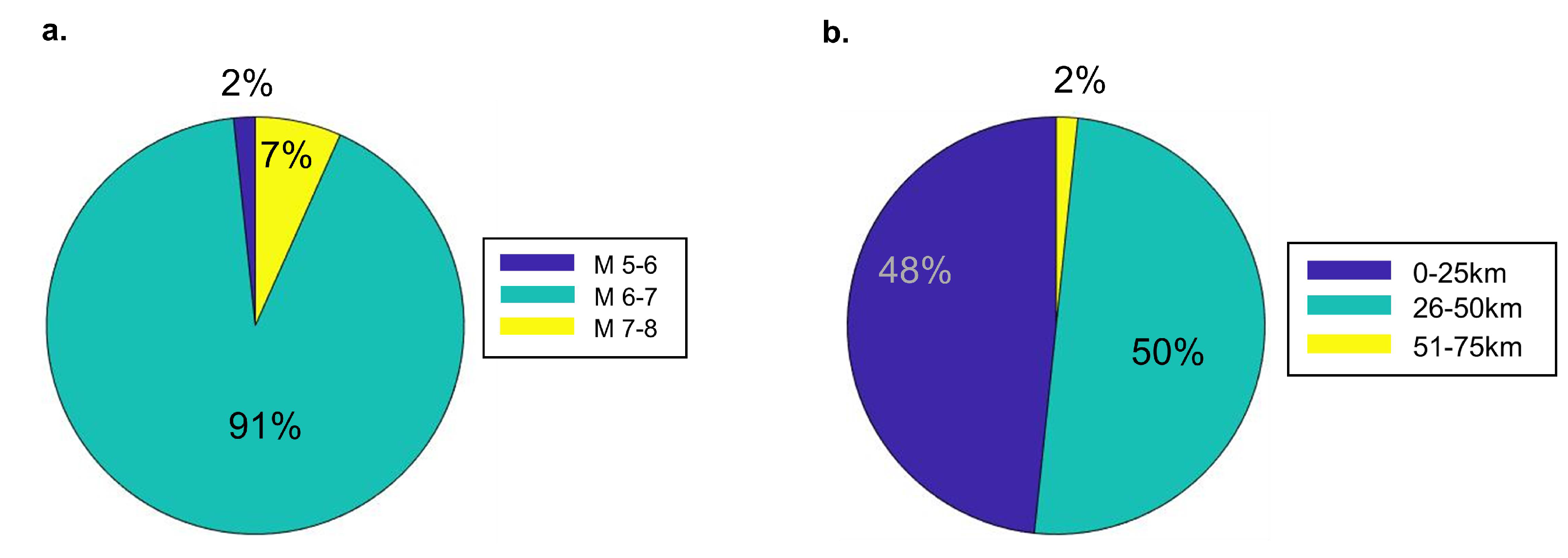
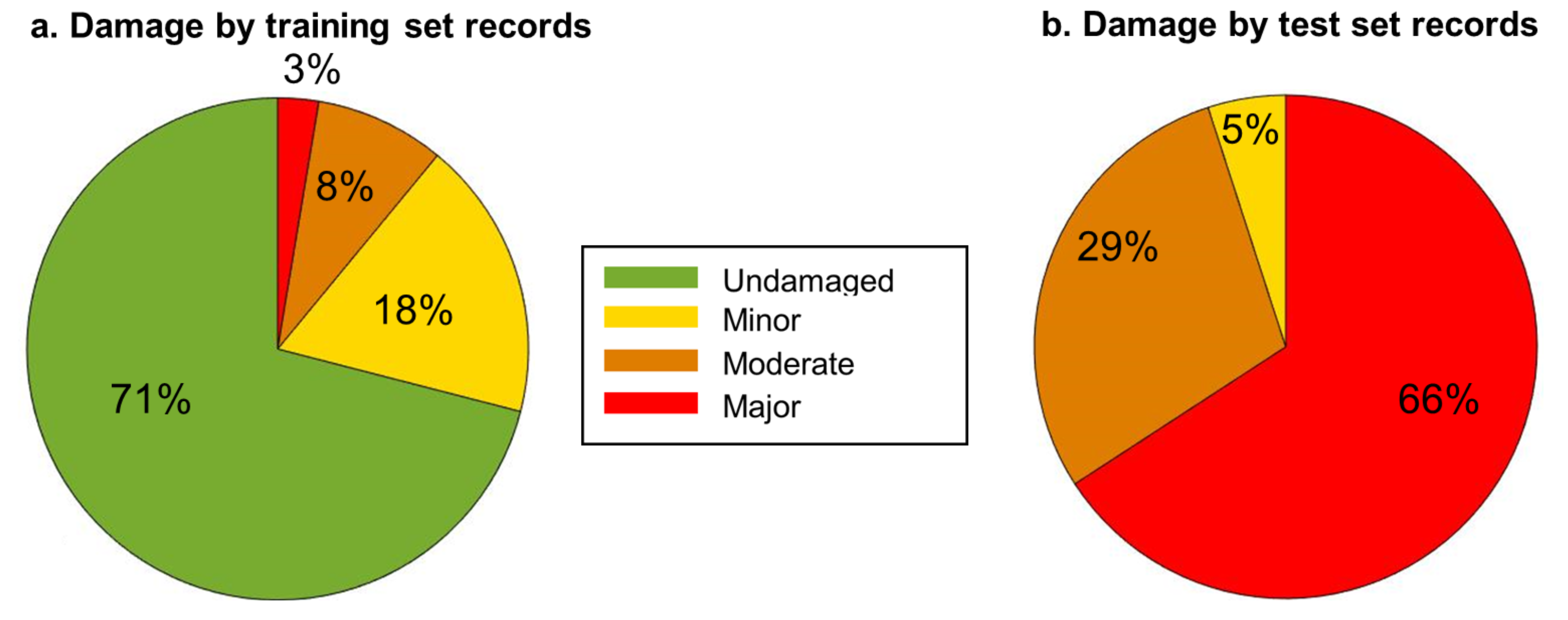
NTHA is performed on the models using both Set-1 and Set-2 records described in Section 2.1.2. The acceleration was computed at each node along with the force and displacement for each spring element. Damage state was evaluated using Equation (1) for each story. The worst damage state among the five stories was assigned as the damage state of the entire building and its location was assigned as the worst damage location. For the cases when the worst damage state occurred simultaneously at several locations, the lowest story was identified as the damage location. For the MDOF-US model, out of the 1710 cases, 1376 (80%), 150 (9%), 133 (8%), and 51 (3%) cases were respectively undamaged, minor damage, moderate damage, and major damage (Figure 7). For the MDOF-NS model, 1382 (81%), 55 (3%), 86 (5%), and 187 (11%) cases were respectively undamaged, minor damage, moderate damage, and major damage (Figure 7). The higher percentage of major damage in MDOF-NS was due to the non-uniform distribution of its shear capacity. The location of the worst damage for MDOF-US was the first story for all the 334 damaging events. In the case of MDOF-NS, damage locations of the 328 damaging events were distributed among all the bottom four stories (no damage was observed in the fifth story) but the majority of the damage locations were in the first and third stories. As previously discussed, the MDOF-US had a conservative design of uniform strength throughout the height. Therefore, the damage in this system occurred sequentially from bottom to top, i.e., the damage initiated at the first story and then moved up. For this reason, the extent of damage decreased with height for MDOF-US. However, for MDOF-NS, the strength variation resulted in concurrent damage at different stories, i.e., in many cases, the damage initiated at the second or third stories.

The features ($CAV,R_{CAV}$) and the ML approach (OLR algorithm) identified in the previous section were utilized to detect the location and severity of damage of the MDOF-US and MDOF-NS models. The $CAV$ of the first story was chosen where the earthquake force demand is expected to be the highest and the $R_{CAV}$ of the top story was selected as it is expected to capture the impact of damage at all lower stories. Moreover, in practice, the ground floor and roof of buildings are usually instrumented. Thus, using features associated with these two stories would be useful for direct applications to instrumented buildings. Using these features, the OLR was trained with TR-1 and tested against TE-1 and TE-2 for both MDOF-US and MDOF-NS with damage categories defined similar to the SDOF system.

Damage location was determined based on the assigned damaged state, i.e., the story that experienced the worst damage state was identified as the damage location. Using the damage state and location information obtained from the training set, the probability of the location of damage for a given damage state $P\left(n\right|y)$ was calculated where n is the story number, i.e., $n=1,\dots ,5$ and y is the damage state, i.e., $y=1,2,3$ ($y=0$ corresponds to the undamaged state). The probabilities of the worst damage location were subsequently determined by Equation (21) for all five stories. The story with the highest $P\left(n\right)$ was considered as the damage location. Here, $P(y=i)$ was obtained using Equations (11)–(14).

$$P\left(n\right)=\sum _{i=1}^{3}P\left(n\right|y=i)\times P(y=i)$$

(21)

4.1.2. Results

Table 4. Damage state and location accuracy (%) for the two MDOF models.

Task	Test Set	MDOF-US	MDOF-NS
Damage State	TE-1	90.67	90.67
	TE-2	84.33	96.67
Location	TE-1	97.50	93.00
	TE-2	97.50	95.00

shows the damage state and location accuracy values for the two MDOF models. Results reveal that MODF-US achieved damage state detection accuracy of 91% and 84% when tested with TE-1 and TE-2, respectively. The higher accuracy with TE-1 was expected since the test set came from the same distribution as the training set. The damage state detection accuracy for MDOF-US and MDOF-NS (91%) tested with TE-1 significantly improved to 97% for MDOF-NS when tested with TE-2.

Although accuracy is a widely used performance metric for ML models, other metrics can further explain the results, e.g., the recall value. Herein, the recall is defined as the proportion of the actual damages identified correctly for each damage state. The closer the recall value to 1, the better the performance of the model. The recall value for the undamaged state was computed using Equation (22).

$${\mathrm{Recall}}_{\mathrm{undamaged}}=\frac{\mathrm{TU}}{\mathrm{TD}1+\mathrm{TD}2+\mathrm{TD}3}$$

(22)

where TU = true undamaged cases, TD1 = true minor damage cases, TD2 = true moderate damage cases, and TD3 = true major damage cases. Similarly, recall values were calculated for the other damage states.

Table 5. Class-specific recall values for the two MDOF models.

Class	MDOF-US	MDOF-NS
Undamaged	0.993	0.993
Minor	0.286	0.000
Moderate	0.781	0.463
Major	0.922	0.966

presents the class-specific recall values for the two MDOF systems. From this table, it is evident that for MDOF-US, the model predicted very well the undamaged class (0.99) and the major damage class (0.92). For moderate damage, it did fairly with a 0.78 recall value. However, minor damage was mostly misclassified due to the definition of the damage states. Since minor damage was defined as $1\le \mu \le 2$, with this narrow range, the model performed poorly to detect minor damages which was further worsened by the lack of data from minor damage states. Similar performance of the model was observed for MDOF-NS. Major damage class had a higher recall value (0.97) than the MDOF-US, because of more data available for this damage state. Both MDOF-US and MDOF-NS had the same recall for the undamaged class.

Table 4 also shows that damage locations were detected with 97.5% accuracy for MDOF-US with both TE-1 and TE-2. It is noted that three inaccurate cases were detected where the worst damage took place in both first and second stories, i.e., the first story was labeled as the correct location, but the model only identified the second story as the worst damage location. The damage locations were detected with 93% and 95% accuracy with TE-1 and TE-2, respectively, for MDOF-NS. Damage location detection for this model was more critical since the non-uniformity of stiffness introduced significant uncertainty about the damage locations. Thus, the results show that the damage location was identified with high confidence, even for non-uniform structural properties, using the proposed method.

4.2. Tai-Tung Fire Bureau Building

4.2.1. Building Description

In this section, OLR was implemented with the $CAV$ and $R_{CAV}$ as features on Tai-Tung Fire Bureau (TFB) building located at Tai-Tung city in Taiwan. TFB was a four-story reinforced concrete building with a partial basement. The first story height for the building was 5 m (16.4 ft) which was taller than the other stories, 3.5 m (11.4 ft). Furthermore, the first story had fewer partition walls for the purpose of parking fire engines and other large equipment causing the first story to behave as a soft story. TFB was instrumented with 22 accelerometers located as shown in Figure 8. It experienced five earthquakes, listed in

Table 6. Earthquake events recorded by the sensors of TFB building.

Event #	Date (mm/dd/yyyy)	Magnitude
1	8/4/1999	4.8
2	9/24/2002	5.2
3	12/10/2003	6.4
4	12/28/2005	4.7
5	4/1/2006	6.2

, and suffered from severe damage during the 2006 M 6.2 earthquake (#5 in Table 6). Several columns of the first story and partition walls on first and second stories experienced major damage. The building was deemed not feasible to repair and was subsequently demolished.

Two MDOF analytical models were developed to simulate the behavior of the lateral force resisting systems in the two directions (X and Y shown in Figure 8) based on details (period, stiffness, damping, etc.) found in [47]. The vibration responses from NTHA of the MDOF models to Set-1 ground motions described in Section 2.1.2 were used to extract damage features and the corresponding damage states. Two training sets of features were generated for the two directions which were subsequently used to develop two OLR models (OLR_X and OLR_Y). For the test sets, the recorded responses of sensors 7, 9, 16, & 19 were used as Test set-1, to evaluate OLR_X, and responses of sensors 8, 10, 17, & 20 were used as Test set-2, to evaluate OLR_Y, where ground floor $CAV$ and roof $R_{CAV}$ were paired as features. Three classification tasks were performed using these data sets, namely binary damage detection, multi-class damage assessment, and damage location detection making use of Equation (21) in this practical application.

4.2.2. Results

Table 7. Damage detection, assessment, and location identification tasks accuracy (%) for TFB Building.

	Damage Detection	Damage Assessment	Damage Location
Test set-1	90.0	80.0	66.7
Test set-2	80.0	70.0	50.0

presents the accuracy values for the three tasks performed showing higher values for Test set-1 than Test set-2. The models performed well for damage detection with respective 90% and 80% accuracy values. Both OLR models had labeled event #3 as a damaged case. This is interesting because even though there was no reported visual damage for event #3, Chu and Lo [48] stated the possibility of nonlinearity during this event. For the damage assessment task, the accuracy values for Test set-1 and Test set-2 were 80% and 70%, respectively. The OLR_X model accurately detected the severe damage state (major damage as described in Section 2.1.3) of event #5 for sensor 19. It labeled the damage state of sensor 16 as moderate (moderate damage as described in Section 2.1.3) and indicated that damage was present for event #3. OLR_Y assessed the damage state of event #5 for sensor 20 as moderate and detected minor damage for event #3.

Figure 9 presents the confusion matrix for the two test sets to better understand the performance of OLR_X and OLR_Y models. It shows OLR_X correctly detected all the damaged responses as damaging. However, it misclassified one response from event #3 as damaged. On the other hand, OLR_Y misclassified both damaged and undamaged responses falsely labeling one of the responses of event #5 as undamaged. Hence, the accuracy for this model was lower compared to OLR_X for both the damage detection and damage assessment tasks.

For damage location, the first story had been identified as the location of the damage for event #5 which was consistent with the observed damages [48]. Per Equation (21), the location was determined for any sample indicating damage. Hence, the model determined damage on the first story for event #3. This reduced the location detection accuracy values for both OLR_X and OLR_Y models to 67% and 50%, respectively (Table 7). As stated before, no visible damage had been identified for event #3 but the present study provided further evidence that the structure was most probably weakened by event #3 and became vulnerable to damage for subsequent earthquake events, especially #5 listed in Table 6.

5. Discussions and Conclusions

In this paper, a rapid damage assessment methodology is presented that uses ML algorithms with single dimension CAV based features. A computer experiment was performed to identify the appropriate features and the ML algorithm using data from a simulated SDOF system. Results from this experiment revealed that $CAV$ and $R_{CAV}$ pair as the ideal feature combination. Not only this combination produced the highest accuracy with all ML tools but also produced the highest accuracy when tested against a dataset different from the training set. Moreover, among the considered four ML algorithms, OLR performed the best for its generalization capabilities.

The presented rapid damage assessment methodology was subsequently applied on two MDOF models and one instrumented building. For the two MDOF models, namely MDOF-US and MDOF-NS, detections of the damage state and location were assessed. The study showed that the proposed method correctly detected the worst damage state with about 91% accuracy for both MDOF models when tested with TE-1. Moreover, it achieved damage state accuracy of 84% and location accuracy of 97.5% for MDOF-US and damage state accuracy of 97% and location accuracy of 95% for MDOF-NS when tested with TE-2. This shows that the proposed method can detect and assess damage even if datasets come from distributions different from the training dataset. However, from the recall values, it was evident that the method was more successful in detecting undamaged and major damage classes than moderate or minor damage classes. The proposed method did exceedingly well in damage location detection even when the locations were fairly distributed among different stories.

For the instrumented building, the training sets came from the analytical models of the lateral force resisting systems of the building. Test sets were the recorded earthquake data of two perpendicular directions. Results showed that damage detection accuracy was 90% and 80% for the two test sets and their corresponding models using OLR. Further investigation of the accuracy values revealed the possibility of undetected damages in one of the earthquake events that made the structure vulnerable to the subsequent damaging earthquake events.

Rapid and accurate monitoring of structures is vital for decision making tasks regarding re-occupancy, emergency response, and future use of the structure following an earthquake event. The techniques reported in this study achieve these tasks via instantaneous use of the response data (simulated and/and measured) to locate and assess the structural integrity. The major challenge in the application of the proposed technique comes from the lack of recorded data as well as the lack of detailed analytical models. A resilient performance in the face of natural hazards can be achieved when all buildings in a community are instrumented to record and transfer strong motion data and have fairly detailed analytical models, i.e., when digital twins are developed and validated. The current developments in sensor technologies, high-performance computing, and wireless data communication open the door to resolve this challenge.

References

1. ASCE. Report Card for California’s Infrastructure. 2021. Available online: https://infrastructurereportcard.org/cat-item/bridges/ (accessed on 20 May 2021).
2. Farrar, C.R.; Worden, K. Structural Health Monitoring: A Machine Learning Perspective; Wiley: Hoboken, NJ, USA, 2012. [Google Scholar]
3. Arici, Y.; Mosalam, K.M. System identification of instrumented bridge systems. Earthq. Eng. Struct. Dyn. 2003, 32, 999–1020. [Google Scholar] [CrossRef]
4. Arici, Y.; Mosalam, K.M. Modal identification of bridge systems using state-space methods. Struct. Control Health Monit. 2005, 12, 381–404. [Google Scholar] [CrossRef]
5. Arici, Y.; Mosalam, K.M. Statistical significance of modal parameters of bridge systems identified from strong motion data. Earthq. Eng. Struct. Dyn. 2005, 34, 1323–1341. [Google Scholar] [CrossRef]
6. Pandey, A.K.; Biswas, M.; Samman, M.M. Damage detection from changes in curvature mode shapes. J. Sound Vib. 1991, 145, 321–332. [Google Scholar] [CrossRef]
7. Zou, Y.; Tong, L.; Steven, G.P. Vibration-based model-dependent damage (delamination) identification and health monitoring for composite structures—A review. J. Sound Vib. 2000, 230, 357–378. [Google Scholar] [CrossRef]
8. Pastor, M.; Binda, M.; Harčarik, T. Modal assurance criterion. Procedia Eng. 2012, 48, 543–548. [Google Scholar] [CrossRef]
9. Chang, K.C.; Kim, C.W. Modal-parameter identification and vibration-based damage detection of a damaged steel truss bridge. Eng. Struct. 2016, 122, 156–173. [Google Scholar] [CrossRef]
10. Brehm, M.; Zabel, V.; Bucher, C. An automatic mode pairing strategy using an enhanced modal assurance criterion based on modal strain energies. J. Sound Vib. 2010, 329, 5375–5392. [Google Scholar] [CrossRef]
11. Todorovska, M.I.; Trifunac, M.D. Earthquake damage detection in the Imperial county services building I: The data and time-frequency analysis. Soil Dyn. Earthq. Eng. 2007, 27, 564–576. [Google Scholar] [CrossRef]
12. Muin, S.; Mosalam, K.M. Localized Damage Detection of CSMIP Instrumented Buildings using Cumulative Absolute Velocity: A Machine Learning Approach. In Proceedings of the SMIP18 Seminar on Utilization of Strong-Motion Data, Sacramento, CA, USA, 25 October 2018. [Google Scholar]
13. Muin, S.; Mosalam, K.M. Cumulative Absolute Velocity as a Local Damage Indicator of Instrumented Structures. Earthq. Spectra 2017, 33, 641–664. [Google Scholar] [CrossRef]
14. Sajedi, S.O.; Liang, X. Vibration-based semantic damage segmentation for large-scale structural health monitoring. Comput. Aided Civ. Infrastruct. Eng. 2019, 35, 579–596. [Google Scholar] [CrossRef]
15. Campbell, K.; Bozorgnia, Y. Use of cumulative absolute velocity (CAV) in damage assessment. In Proceedings of the 15th World Conference on. Earthquake Engineering, Lisbon, Portugal, 24–28 September 2012; pp. 1–10. [Google Scholar]
16. Zengin, E.; Abrahamson, N.A. A vector-valued intensity measure for near-fault ground motions. Earthq. Eng. Struct. Dyn. 2020, 49, 716–734. [Google Scholar] [CrossRef]
17. Muin, S.; Mosalam, K.M. Human-Machine Collaboration Framework for Structural Health Monitoring and Resiliency. Eng. Struct. 2021, 235, 112084. [Google Scholar] [CrossRef]
18. Lam, H.F.; Yuen, K.V.; Beck, J.L. Structural health monitoring via measured Ritz vectors utilizing artificial neural networks. Comput. Aided Civ. Infrastruct. Eng. 2006, 21, 232–241. [Google Scholar] [CrossRef]
19. Figueiredo, E.; Park, G.; Farrar, C.R.; Worden, K.; Figueiras, J. Machine learning algorithms for damage detection under operational and environmental variability. Struct. Health Monit. 2011, 10, 559–572. [Google Scholar] [CrossRef]
20. Abdul-Aziz, A.; Woike, M.R.; Oza, N.C.; Matthews, B.L.; Lekki, J.D. Rotor health monitoring combining spin tests and data-driven anomaly detection methods. Struct. Health Monit. 2012, 11, 3–12. [Google Scholar] [CrossRef]
21. Ng, C.T. Application of Bayesian-designed artificial neural networks in Phase II structural health monitoring benchmark studies. Aust. J. Struct. Eng. 2014, 15, 27–36. [Google Scholar] [CrossRef] [Green Version]
22. Bakhary, N.; Hao, H.; Deeks, A.J. Substructuring technique for damage detection using statistical multi-stage artificial neural network. Adv. Struct. Eng. 2010, 13, 619–639. [Google Scholar] [CrossRef]
23. Hakim, S.; Razak, H.A.; Ravanfar, S. Fault diagnosis on beam-like structures from modal parameters using artificial neural networks. Measurement 2015, 76, 45–61. [Google Scholar] [CrossRef]
24. Jiang, S.F.; Zhang, C.M.; Yao, J. Eigen-level data fusion model by integrating rough set and probabilistic neural network for structural damage detection. Adv. Struct. Eng. 2011, 14, 333–349. [Google Scholar] [CrossRef]
25. Pawar, P.M.; Venkatesulu Reddy, K.; Ganguli, R. Damage detection in beams using spatial Fourier analysis and neural networks. J. Intell. Mater. Syst. Struct. 2007, 18, 347–359. [Google Scholar] [CrossRef]
26. Mehrjoo, M.; Khaji, N.; Moharrami, H.; Bahreininejad, A. Damage detection of truss bridge joints using artificial neural networks. Expert Syst. Appl. 2008, 35, 1122–1131. [Google Scholar] [CrossRef]
27. Abdeljaber, O.; Avci, O.; Kiranyaz, M.S.; Boashash, B.; Sodano, H.; Inman, D.J. 1-D CNNs for structural damage detection: Verification on a structural health monitoring benchmark data. Neurocomputing 2018, 275, 1308–1317. [Google Scholar] [CrossRef]
28. Khodabandehlou, H.; Pekcan, G.; Fadali, M.S. Vibration-based structural condition assessment using convolution neural networks. Struct. Control Health Monit. 2019, 26, e2308. [Google Scholar] [CrossRef]
29. Gui, G.; Pan, H.; Lin, Z.; Li, Y.; Yuan, Z. Data-driven support vector machine with optimization techniques for structural health monitoring and damage detection. KSCE J. Civ. Eng. 2017, 21, 523–534. [Google Scholar] [CrossRef]
30. Ghiasi, R.; Torkzadeh, P.; Noori, M. A machine-learning approach for structural damage detection using least square support vector machine based on a new combinational kernel function. Struct. Health Monit. 2016, 15, 302–316. [Google Scholar] [CrossRef]
31. Pan, H.; Azimi, M.; Yan, F.; Lin, Z. Time-frequency-based data-driven structural diagnosis and damage detection for cable-stayed bridges. J. Bridge Eng. 2018, 23, 04018033. [Google Scholar] [CrossRef]
32. McKenna, F. OpenSees User’s Manual. 2010. Available online: http://opensees.berkeley.edu (accessed on 20 August 2018).
33. Mahin, S.; Lai, J.W.; Wang, S.; Schoettler, M. Evaluating and improving the seismic performance of older tall buildings. In Proceedings of the Second International Conference on Performance-Based and Life-Cycle Structural Engineering, Brisbane, Australia, 9–11 December 2015; The University of Queensland: St Lucia, Australia, 2015; pp. 25–37. [Google Scholar]
34. Günay, S.; Mosalam, K.M. Acceleration Response Spectrum: Revisited for Higher Mode Effects. In Proceedings of the 16th World Conference on Earthquake, Santiago, Chile, 9–13 January 2017. [Google Scholar]
35. International Code Council (ICC). International Building Code; International Code Council: Washington, DC, USA, 2012. [Google Scholar]
36. Bozorgnia, Y.; Abrahamson, N.A.; Atik, L.A.; Ancheta, T.D.; Atkinson, G.M.; Baker, J.W.; Baltay, A.; Boore, D.M.; Campbell, K.W.; Chiou, B.S.J.; et al. NGA-West2 research project. Earthq. Spectra 2014, 30, 973–987. [Google Scholar] [CrossRef] [Green Version]
37. Pacific Earthquake Engineering Research Center (PEER). NGA West2 Database. 2020. Available online: https://ngawest2.berkeley.edu/ (accessed on 17 February 2020).
38. Baker, J.W.; Lin, T.; Shahi, S.K.; Jayaram, N. New Ground Motion Selection Procedures and Selected Motions for the PEER Transportation Research Program; Peer Report 2011/3; Pacific Earthquake Engineering Research Center: Berkeley, CA, USA, 2011. [Google Scholar]
39. Applied Technology Council for the Federal Emergency Management Agency. Seismic Performance Assessment of Buildings: 1—Methodology; Applied Technology Council for the Federal Emergency Management Agency: Redwood City, CA, USA, 2012. [Google Scholar]
40. Reed, J.W.; Kassawara, R.P. A criterion for determining exceedance of the operating basis earthquake. Nucl. Eng. Des. 1990, 123, 387–396. [Google Scholar] [CrossRef] [Green Version]
41. Bommer, J.J.; Martinez-Pereira, A. The effective duration of earthquake strong motion. J. Earthq. Eng. 1999, 3, 127–172. [Google Scholar] [CrossRef]
42. Alibrandi, U.; Muin, S.; Mosalam, K.M. The method of the independent components for sustainable building design. In Proceedings of the 2015 IEEE International Conference on Building Efficiency and Sustainable Technologies (ICBEST), Singapore, 31 August 2015; pp. 101–106. [Google Scholar]
43. Muin, S.; Günay, S.; Mosalam, K.M. Decision making of innovative building façade use in Singapore. In Proceedings of the Second International Conference on Performance-Based and Life-Cycle Structural Engineering, Brisbane, Australia, 9–11 December 2015; The University of Queensland: St Lucia, Australia, 2015; pp. 1278–1286. [Google Scholar]
44. Schmidhuber, J. Deep learning in neural networks: An overview. Neural Netw. 2015, 61, 85–117. [Google Scholar] [CrossRef] [PubMed] [Green Version]
45. Miranda, E.; Reyes, C.J. Approximate lateral drift demands in multistory buildings with nonuniform stiffness. J. Struct. Eng. 2002, 128, 840–849. [Google Scholar] [CrossRef]
46. American Society of Civil Engineers. Minimum Loads and Associated Criteria for Buildings and Other Structres; American Society of Civil Engineers: Reston, VA, USA, 2016. [Google Scholar]
47. Wang, J.F.; Lin, C.C.; Lin, G.L.; Yang, C.H. Story damage identification of irregular buildings based on earthquake records. Earthq. Spectra 2013, 29, 963–985. [Google Scholar] [CrossRef]
48. Chu, S.Y.; Lo, S.C. Application of the on-line recursive least-squares method to perform structural damage assessment. Struct. Control Health Monit. 2011, 18, 241–264. [Google Scholar] [CrossRef]
Figure 1. Proposed framework using acceleration data from instrumented structures to assess their damage conditions following an earthquake event.
Applsci 11 05727 g001
Figure 2. (a) Magnitude and (b) distance of Set-1 (ground motions from PEER NGA-West2).
Applsci 11 05727 g002
Figure 3. (a) Magnitude and (b) distance of Set-2 (ground motions from [38]).
Applsci 11 05727 g003
Figure 4. Damage states of the SDOF system produced by records from (a) Set-1 and (b) Set-2.
Applsci 11 05727 g004
Figure 5. Plots of the relationships of the proposed features and the displacement ductility.
Applsci 11 05727 g005
Figure 6. (a) MDOF models used in the study, (b) Story shear distribution along the height, (c) Story force-displacement relationship [34].
Applsci 11 05727 g006
Figure 7. Worst damage state and location distribution of the MDOF-US and MDOF-NS models.
Applsci 11 05727 g007
Figure 8. Sensor locations at TFB building.
Applsci 11 05727 g008
Figure 9. Confusion matrices for two test sets of TFB building to evaluate (a) OLRX and (b) OLRY.
Applsci 11 05727 g009