Understanding Natural Disaster Scenes from Mobile Images Using Deep Learning

Abstract

With the ubiquitous use of mobile imaging devices, the collection of perishable disaster-scene data has become unprecedentedly easy. However, computing methods are unable to understand these images with significant complexity and uncertainties. In this paper, the authors investigate the problem of disaster-scene understanding through a deep-learning approach. Two attributes of images are concerned, including hazard types and damage levels. Three deep-learning models are trained, and their performance is assessed. Specifically, the best model for hazard-type prediction has an overall accuracy (OA) of 90.1%, and the best damage-level classification model has an explainable OA of 62.6%, upon which both models adopt the Faster R-CNN architecture with a ResNet50 network as a feature extractor. It is concluded that hazard types are more identifiable than damage levels in disaster-scene images. Insights are revealed, including that damage-level recognition suffers more from inter- and intra-class variations, and the treatment of hazard-agnostic damage leveling further contributes to the underlying uncertainties.

1. Introduction

Disasters are a persistent threat to human well-being, and disaster resilience is of paramount importance to the public. To achieve disaster resilience, technical and organizational resources play vital roles in securing adequate preparation, adaptable response, and rapid recovery [1]. During the phases of response and recovery, while disaster scenes are possibly still being unfolded, information collection via disaster reconnaissance is crucial for restoring the functionalities of communities and infrastructure systems. Disaster scenes, however, are perishable as a disaster recedes and recovery efforts progress. Traditional remote sensing (RS) technologies via orbital or airborne imaging sensors have long been recognized as a helpful tool that provides geospatial analytics for improving the efficacy of disaster reconnaissance. In general, RS technologies can provide data that record the disaster scenes, including unfolded hazards (e.g., flood inundation) and disastrous consequences (e.g., building damage). However, traditional RS platforms suffer from long time latency due to revisit periods, orbital maneuver, and the ensuing data processing [2]. Moreover, due to their orbital or airborne view, it is often impossible for traditional RS sensors to capture the elevation view of built objects (e.g., buildings) and other detailed structural conditions. Therefore, although it is less efficient in terms of spatial coverage, ground-based disaster reconnaissance is not replaceable by traditional remote sensing.

In recent years, two emerging RS technologies are changing the normal of disaster reconnaissance. First, due to the ubiquity of digital cameras, smartphones, body-mounted recording devices, and social networking smart apps, which may be collectively termed smart devices, can seamlessly capture, process, and share images. This nearly real-time imaging can record personal and public events, including disasters. Many researchers in Civil Engineering hence recognize the power of mobile devices for aiding disaster response, infrastructure inspection, and construction monitoring [3,4,5,6]. The second is the use of small unmanned aerial vehicles (UAVs). As witnessed in recent years, since UAVs can provide high-resolution coverage of ground scenes at low above-ground-level (AGL) heights, many research efforts investigate the application of UAV-based RS [7,8,9,10]. UAV imaging can be deployed with diverse modes, including survey-grade imaging similar to traditional airborne remote sensing.

Nonetheless, recent trends include using a micro-sized UAV as a flying camera at a very low AGL, which is then similar to the imaging with the use of mobile devices, for example, via the so-called ‘follow-me’ drone [11]. In this paper, the authors propound that this non-traditional RS practice can conduce to the demand for real-time analytics arising from the post-disaster response and recovery activities. By recognizing their primary characteristic of using small and low-cost devices carried or operated by human users or operators, the term mobile remote sensing is coined in this effort. It is noted that in this paper, the emphasis is on smart device-based imaging and the disaster-scene images from this venue. In the meantime, this choice is supported by the abundance of such images, as researchers have archived a large volume of mobile imagery data from numerous disaster reconnaissance activities (e.g., as found in DesignSafe-CI, a collaborative cloud-based workspace) [12].

Mobile RS provides untapped opportunities for extracting relevant information and understanding natural disasters. However, significant differences exist when comparing the processing methods for mobile RS images against traditional ones. First, traditional RS images are generally ortho-rectified and geo-referenced when provided for processing and understanding. Because of such geo-readiness, many application efforts concern change detection, which is to detect landscape differences at different times for a terrain of interest on the Earth surface. As such, besides basic photogrammetric processing methods, a wide range of digital change-detection methods are found [13,14,15,16,17]. Mobile RS images differ from traditional ones in that they are often opportunistically collected. Due to their low-altitude or ground-level capturing mode, numerous images at different perspective angles are necessary for characterizing a local scene. Therefore, the involved processing to obtain a full view of the object (e.g., via a 3-dimensional reconstruction process) is much more complex than processing geo-ready images. Second, although mobile RS images can be geo-tagged via geographical positioning services in smart devices, many social or crowdsourced images are often marked with questionable geo-tags or simply have not geo-tags [18,19]. Last, traditional RS images captured at different times can give rise to a time-series coverage for a particular region, whereas mobile RS data lacks such temporal advantages. These differences imply that one cannot use the traditional photogrammetric processing and change-detection methods to deal with mobile RS images that are arranged spatially and temporally non-structural. From this point of view, the process of processing and understanding mobile RS images, including extraction, interpretation, and localization of objects in images, belong to the general image understanding problem as defined in the computer or machine vision literature [20,21]. By borrowing this concept, image-based disaster-scene understanding is coined in this paper, which is defined as a computational process of extracting information and detecting features or objects from images relevant to interpret a disaster. As will be further elaborated, research gaps exist towards a more cognitive mobile RS-based disaster-scene understanding.

This paper contributes to the knowledge by developing and testing a deep-learning framework to understand disaster scenes. In this framework, the proposed learning models identify two essential properties in a given disaster image (namely the hazard type and the disaster-induced damage level). Performance evaluation reveals the insights in understanding disaster scenes in mobile images, including that the general damage-level classification is more challenging than hazard-type recognition. To achieve the goal, the authors built a multi-hazard disaster database with images from multiple sources, which forms another contribution of this paper. In the following, the specific research problems and challenges are defined. The methodology framework is proposed, including data preparation, network architectures and adjustment for two deep-learning models, and transfer-learning-based training. Three strategically designed deep-learning models are evaluated in this paper, followed by a comprehensive discussion. Conclusions are then given based on the research findings in this paper.

2. Research Problems and Challenges

Disaster scenes from extreme events, such as hurricanes, floods, earthquakes, tsunamis, and tornadoes, are considerably complex. From the perspective of naked eyes, a disaster scene includes countless visual patterns related to built objects, natural hazards, landscapes, human activities, and many others. The semantic attributes for labeling patterns relevant to this effort are named hazard-type and damage-level. The rationale for this proposition is justified as follows by examining the practice of professional reconnaissance activities.

It is a cognitive process when professionals in a disaster field conduct digital recording via cameras or smart apps, e.g., Fulcrum [22]. To the trained eyes of professional engineers, their attention can be quickly paid to the visual patterns of interest, the built objects, the apparent damage features (e.g., cracking or debris), and other clues that are relevant to damage due to the extraordinary intelligence of human beings and their professional training. For example, a post-tsunami image often contains inundation marks or water-related textures, whereas the post-earthquake images usually show conspicuous cracking in buildings or cluttered debris. For tornado scenes, the damaging effects usually lie on the roof or the upper area of buildings, showing peeled surface materials due to wind blowing and shearing. In sum, professionals often act as a detective while conducting a forensic engineering process. In this process, they record the consequential evidence of damage in built objects using digital images. They further look for cues that cause the damage, namely the causal evidence of hazardous factors, which may co-exist in the same image of damaged objects or are recorded in different images. Second, this cognitive process continues in written reports by professionals, where the images are often showcased with captions or descriptions. Domain knowledge is more involved in this process, wherein the engineers tend to use a necessary number of images to analyze the common evidence of hazards and damage in images, then remark the intensity of the hazard and the degree of damage rationally, and even further, infer the underlying contributing factors, such as structural materials and geological conditions. Indeed, this has been called a learning from disaster in engineering communities as demonstrated in many disaster reconnaissance reports (e.g., [23]).

This cognitive understanding and learning process rarely occurs when the crowd conducts it as they lack domain knowledge. Also, even it is conducted by professionals, they may seek to excessively record disaster scenes yet without describing and reporting all images. As mentioned earlier, digital archives and social networks to this date have stored a colossal volume of images recording extreme events in recent years, which are not exploited or analyzed in the foreseeable future. This accumulation will inevitably be explosive with the advent of ubiquitous use of personal RT devices, for example, body-mounted or flying micro-UAV cameras.

In this paper, inspired by the practical cognitive process of disaster-scene understanding, the authors argue an identifiable causality pair in a disaster-scene image, the hazard applied to and the damage sustained by built objects in images. This identifiable causality, more specifically termed disaster-scene mechanics, gives rise to the fundamental research question in this effort: does a computer-vision-based identification process exist that can process and identify hazard and damage related attributes in a disaster-scene image? To accommodate a computer-vision understanding process, the attributes are reduced to be categorical. As such, two identification tasks are defined in this paper:

(1)

Given a disaster-scene image, one essential task is to recognize the contextual and causal property embedded in the image, namely the Hazard-Type.

(2)

The ensuing identification is to estimate the damage-level for an object (e.g., a building).

It is noted that compared with human-based understanding found in professional reconnaissance reports, the underlying intelligence is much reduced in the two fundamental problems defined above. Regardless, significant challenges exist toward the images-based disaster-scene understanding process.

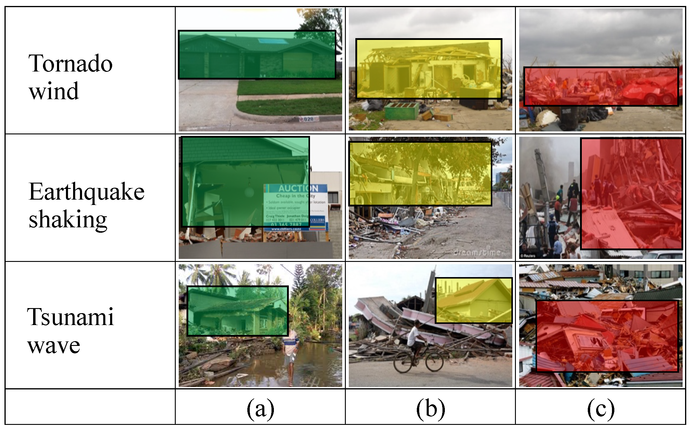
The challenges come from two interwoven factors: the scene complexity and the class variations. To illustrate the image complexity and the uncertainties, sample disaster-scene images are shown in Figure 1, which are manually labeled with hazard-type and damage-level. Observing Figure 1 and other disaster-scene images, the first impression is that image contents in these images are considerably rich, containing any possible objects in natural scenes. Therefore, understanding these images belong to the classical scene understanding problem in Computer Vision [24,25], which is still being tackled today [26]. In terms of variations, as one inspects the image samples in Figure 2, it is relatively easy to distinguish the hazard-type if the images show visual cues of water, debris, building, and vegetation patterns. However, when labeling damage-level, it is observed that the ‘Major’ or ‘Minor’ damage-level is relatively easy to identify, whereas the ‘Moderate’ possess significant uncertainties between different observers or even the same observer at different moments, which are collectively called inter-class variations. As one inspects more images, the variations are extensively observed within images that fall in the same class in terms of either the same hazard-type or damage-level, known as intra-class variations [27]. The effects of these variations are two-fold. First, human-based labeling is more likely to be erroneous, which increases the theoretical lower-bound decision errors. Second, they challenge any machine-learning candidate model if it has a low capacity in representing the complexity or weak discriminative power to deal with the class variations.

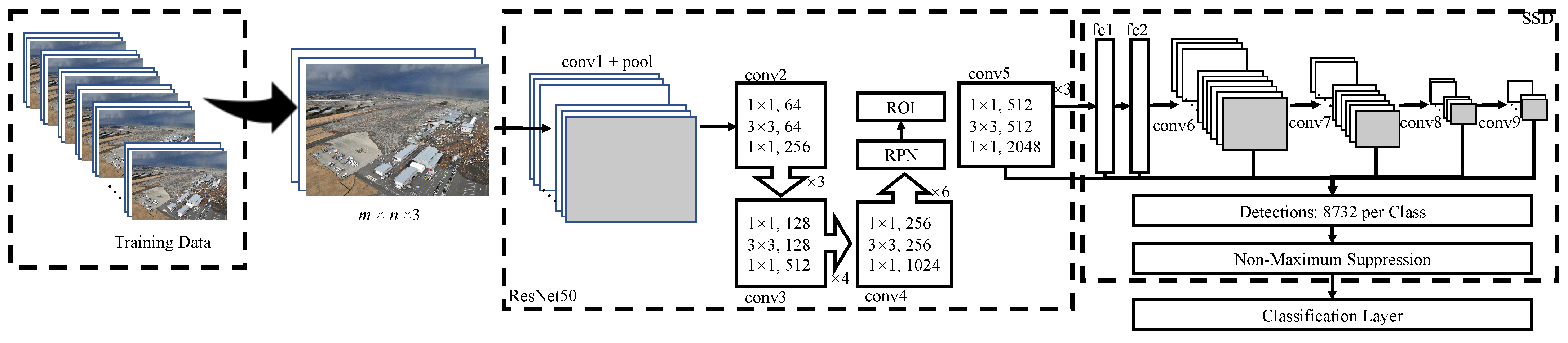
The scene complexity and the conjunct inter-class and intra-class variations pose significant challenges in constructing a supervised learning-based model. Such a model should be high-capacity to encode the complexity in images and be sufficiently discriminative to identify class boundaries in the feature space. By considering these demands, the bounding-box-based object-detection models are selected in this paper. A review of related background is given in the following.

3. Deep-Learning-Based Framework

3.1. Review of Deep Learning

The performance of natural scene understanding culminates today as deep-learning techniques advance [24,25,26]. A deep-learning model, incorporating both feature extraction and classification in an end-to-end deep neural network architecture, can learn intricate patterns (including the objects of interest and the background in images) from large-scale datasets. For visual computing tasks, the dominant deep-learning architecture is the Convolutional Neural Network (CNN), which has a reported superb performance in many types of tasks, such as object classification, localization, tracking, and segmentation [28]. Moreover, contemporary deep-learning models, especially those for image-based scene understanding, possess an advantageous mechanism when learning from small datasets, the transfer learning (TL) mechanism. The technical advantage of TL, briefly speaking, is that if a pre-trained CNN model bearing a priori knowledge of the general scenes via learning from a large-scale database, it can be re-trained over the new but small database to achieve updated knowledge for objects of interest with improved convergence rates and prediction performance [29,30]. In the literature, many commonly used CNN models have been trained and validated based on a large-scale database (e.g., the ImageNet [31]); the backbones of these CNN models (usually all layers except the final classification layer) can be directly used to realize transfer learning in a new model.

In this effort, the central problem of image-based hazard-type and damage-level classification is essentially an object-detection problem, including localization and classification. Early object-detection methods often use sliding-window and template-matching strategies. However, they are superseded by more accurate deep-learning-based methods in recent years. The first category of deep-learning-based methods features bounding-box detection, which provides a natural mechanism of classifying the region of interest in an image domain, namely an attention mechanism. Two strategies are found for bounding-box-based localization of objects: region-proposal strategy represented by the Faster R-CNN model [32] and regression-based generation as in the Single Shot Multibox Detector (SSD) [33]. The third type of object-detection technique aims to localize and classify objects at the pixel level, which is known as semantic segmentation [34]), and is typically much computationally expensive (as shown in [35]). In light of disaster scenes in images, which often show cluttered objects without apparent boundaries, pixel-level segmentation is unnecessary.

The two bounding-box detection models, Faster R-CNN and SSD, are adopted and further modified in this paper; for a detailed comparison and evaluation of the original models, one can refer to a recent review paper [36]. To this date, the Faster R-CNN is a de-facto CNN-based object-detection model, which implements shared network weights and adopts uniform network structures (the Regional Proposal Network, or RPN, and a user-selected CNN for feature extraction), resulting in much faster and more accurate prediction than its predecessors (Fast R-CNN and R-CNN) [32]. It is noted that in a Faster R-CNN model, besides the two core networks (RPN and CNN), bounding-box coordinates regression and final classification layers still exist. On the other hand, the SSD model realizes global regression and classification, mapping straightly from image pixels to bounding-box coordinates and class labels. Therefore, the SSD model remarkably reduces the prediction time and achieves real-time prediction, which was reported to have a rate of 46 frames per second (FPS) compared with about 7 FPS for Faster R-CNN [33]. Nonetheless, as evaluated by [36], its performance gain sacrifices its accuracy in detecting small objects or objects with granular features in images.

3.2. Methodology Framework

In this effort, three deep-learning models are developed and evaluated based on a unique disaster-scene database prepared by the authors. The basic methodological steps are illustrated in Figure 1. In the following, these steps are detailed.

3.2.1. Multi-Hazard Disaster-Scene Database

A multi-hazard disaster-scene (MH-DS) database covering three different hazard types with mobile images captured mostly in urban settings is created in this paper and has been publicized as an open-source database [37]. This database was completed by the authors and several graduate and undergraduate researchers at the University of Missouri–Kansas City. This moderate-scale database, including approximately 1757 color images, was collected from five disaster events worldwide. Among them, 760 images were collected using Internet searching based on two earthquake disasters (the 2010 Haitian earthquake and the 2011 Christchurch Earthquake, New Zealand). Five hundred fifty-six (566) images were searched from the Internet based on two tsunami disasters (the 2011 Tōhoku Earthquake and Tsunami in Japan and the 2004 Indonesian Tsunami). The remaining 441 images were collected and shared by a research team from the 2013 Moore Tornado, Oklahoma [38]. As illustrated in Figure 2, three types of hazardous forces are embedded in the images in accordance with the five disaster events; all images are filtered such that one or multiple buildings are found in the images. It is noted that when developing the disaster-scene database, images with intact or normal buildings without a disaster context are not considered. If otherwise added, the treatment is to add a label of ‘no-damage’ or ‘no-hazard’ to the class labels; in such case, the model to be developed essentially conducts building detection. For solving the research problem in this paper, this is irrelevant.

The semantics creation process for completing the disaster-scene database is introduced below. At the end of this process, besides the original images, two types of metadata are created: the coordinates for a bounding box in the image (four integer values) and the class types for hazard-type and damage-level (two integer values). This process is similarly used as in a typical object-detection-oriented image database in the literature of computer vision. In this paper, it was assisted by using an open-source package, ImageLabel [31]. First, for localizing an object in an image, the most common approach is to annotate a bounding box to the object. Nonetheless, how to define a bounding box that largely expresses the attributes of hazard-type and damage-level is a very subjective process. The authors discover that although cognition is individualistically different, there is an attention zone in each image that attracts a human observer who can collectively determine the hazard-type and damage level, leading to the desired consensus necessary for annotating and labeling images by multiple analysts. It is found too that such attention zones subtly differ between labeling the hazard-type and that for damage-level. For the hazard-type, the features in such a zone include all pertinent objects in an image, including buildings, vegetation, water, pavement, and vehicles. The attention is focused on the damaged buildings due to the secondary task of classifying the damage level. For determining the damage level, the attention zone is mostly on the buildings and their structural failure features. To avoid creating two different bounding boxes for localizing hazard-type and damage-level in an image, only a single bounding box is manually annotated to approximate the underlying building-object focused attention zone. However, the authors argue that this treatment may compromise the model performance.

Following the bounding-box annotation, labels for the hazard type and damage level are assigned to each image. Due to the image collection process, hazard-type recognition and labeling are relatively straightforward. Given the disaster-event type known in advance of the collection process, the analysts only need to filter out images that do not fall in any of the hazard-type. For example, given the 2011 Tōhoku event, buildings damaged by earthquakes were found in images; to focus on the tsunami-wave induced hazards, these images were excluded. When assessing the images from the 2011 Christchurch Earthquake, images with ground water-related scenes (due to liquefaction) were removed. Damage-level recognition and labeling bear more uncertainties. First, no standard or rule can guide damage-level scaling agnostic to hazard types. The most commonly used guide for field-based visual damage scaling is found in [39], which defines five levels of identifiable damage based on visual features of a low-rise building. However, it is for earthquake-induced damage only. In this effort, with five hazard types and considering indefinite variations in building materials and types, three levels of damage are enacted to describe damage-level, which is assumed to be invariant to hazard types and building properties. Consequentially, the authors propose to use the following three damage levels. (1) The ‘Minor’ level stands for slight damage (usually the structure stands and appears to have a few instances of cracks, cluttered objects, or debris); (2) The ‘Moderate’ level describes globally moderate to locally severe damage (visually, the object stands but appears to have many cluttered artifacts, severe cracks, or distorted elements); (3) The ‘Major’ level covers both globally severe damage and full collapse (visually the structure shows partial to full collapse).

A numeric tag is uniquely assigned to simplify the labeling, which differentiates both the hazard type and the damage level. After the manual labeling and bounding-box creation, all these visually obtained manual tagging and annotation results become the critical metadata as an integral part of the resulting disaster-scene database for the ensuing machine-learning framework. Furthermore, the labels and bounding-box information (including the coordinates of the bounding-box corners in images) for each image is written in an XML file. The number of the resulting XML files is the same as the number of images in the database. Figure 3 illustrates the distribution of the resulting labels. It is noted that the instances of class labels are not well-balanced, where the Earthquake type takes $43.5\%$ of all hazard-type class labels, and the Moderate type owns $44.5\%$ of all damage-level labels. This imbalance needs to be heeded when evaluating model performance.

3.2.2. Deep-Learning Models and Training

Given the nature of a disaster scene, it bears two attributes simultaneously: the hazard type and the damage level. Two classification schemes can be designed. First, one can multiply the two sets of class labels, attempting to create a learning model that predicts nine different classes. The problem at hand can be achieved by using a single model outputting nine class labels. The second one is to predict hazard-type and damage-level, separately, by two independent models. In this effort, to achieve straightforward performance evaluation and to reveal the insights about what aspect of the underlying disaster-scene mechanics is identifiable by a computer model, the second scheme is adopted. Accordingly, each of the two disaster-scene attributes is learned separately from the data using a standalone model.

As reviewed and reasoned previously, the generic bounding-box-based object-detection models, Faster R-CNN and SSD, are adopted in this work as the baseline architectures. First, given the flexibility of choosing a user-defined CNN feature extraction in Faster R-CNN, two CNN-based extractors are evaluated, which are the ZF (Zeiler and Fergus) CNN as used in the original Faster R-CNN model in [32], and the ResNet-50, a popular and high-performance extractor proposed by [40]. Second, given the computational gain of using the SSD architecture, a modified SSD model with the ResNet-50 as the feature extractor is developed for comparison with the Faster R-CNN counterpart.

With this treatment and the consideration of two different deep-learning architectures and two CNN-based feature extractors, three different deep-learning models for the two different predictive tasks are designed, trained, and tested in this work, as defined in

Table 1. Disaster-scene learning models and class prediction.

Models	Class 1	Class 2	Class 3
$M_{HT}(FRC,ZF)$	Tornado	Tsunami	Earthquake
$M_{DL}(FRC,ZF)$	Minor	Moderate	Major
$M_{HT}(FRC,RN)$	Tornado	Tsunami	Earthquake
$M_{DL}(FRC,RN)$	Minor	Moderate	Major
$M_{HT}(SSD,RN)$	Tornado	Tsunami	Earthquake
$M_{DL}(SSD,RN)$	Minor	Moderate	Major

Note: HT—hazard-type; DL—damage-level; FRC—Faster R-CNN; RN—ResNet-50; and SSD, Single Shot MultiBox Detector.

. In Table 1, the symbol $M_{HT}$ means to learn hazard-type: $M_{HT}(FRC,ZF)$ using Faster R-CNN with a ZF extractor, $M_{HT}(FRC,RN)$ with ResNet50, and $M_{HT}(SSD,RN)$ using SSD with ResNet50. The model with the symbol $M_{DL}$ outputs the damage level. Similarly, $M_{DL}(FRC,ZF)$ refers to the Faster R-CNN model with ZF, $M_{DL}(FRC,RN)$ means Faster R-CNN with ResNet50 and $M_{DL}(SSD,RN)$ applies the SSD network. Table 1 summarizes the achieved trained models and their goals of prediction. With this attribute separation, Table 1 simplifies the model outputs: for both types of models, Class 1, 2, and 3 correspond to either the three hazard types or the three damage levels, respectively. Therefore, besides the modification as presented in the following, all the models are adapted to output three class labels.

3.2.3. Modified Faster R-CNN Models

As shown in Figure 4, this network consists of two sub-networks: a basic convolutional network for image feature extraction and the region-proposal network for bounding-box prediction. To evaluate the effects of CNN feature extractors, the basic ZF network is used first. As originally proposed in [32], this model is taken as a baseline model in this paper. The ZF network [41], a variant of the AlexNet model, can map the extracted features to a synthesized image at the pixel level (termed DeConvNet), which makes it convenient to visualize the mechanism of CNN-based feature extraction. ZF network has five convolutional layers and two fully connected layers. Figure 4a illustrates this network.

In the second model, the ZF network is replaced by the ResNet-50 [42] as an enhanced feature extractor. In the ResNet family of networks, multiple nonlinear layers are used to approximate a residual function. This treatment significantly reduces the degradation phenomenon caused by introducing deeper layers. The ResNet layers are structured into blocks, and typical block stacks three layers: 1 × 1 convolutional layer for reducing the dimension first, a 3 × 3 convolutional layer, and another 1 × 1 convolutional layer for restoring the dimension. Adopting batch-normalization (BN) in ResNet further enables improved generalization performance for such a large-scale deep network. A ResNet-50 network has four main clustered layers, which have 3, 4, 6, and 3 blocks in each cluster. As a result, ResNet-50 has 50 layers. Since the last layer of ResNet50 is a fully connected layer that cannot directly connect to the RPN stage in the Faster R-CNN architecture, the output from the 3rd layer cluster of ResNet50 is fed to the RPN sub-network. The ROI layer is re-connected to the 4th layer cluster of the ResNet-50, followed by the fully connected layers for bounding-box and label prediction. Figure 4b illustrates the resulting modified Faster R-CNN network.

3.2.4. Modified SSD Network

With the concern of expensive computation pertinent to the Faster R-CNN architecture, the authors further consider the SSD architecture. To have a fair comparison with the Faster R-CNN with a ResNet-50 extractor, ResNet-50 is adopted for the SSD model. This treatment implies that when comparing the Faster R-CNN models with the modified SSD in this paper, the only difference at the architecture level is their individualistic treatment of bounding-box generation and classification scores generation. The resulting architecture of the SSD model is shown in Figure 5.

3.2.5. Training Via Transfer Learning

The disaster-scene database in this work has about 1700 (1.7 K) images for both training and testing. For training and testing in this effort, 85% and 15% of the images are randomly picked, respectively. As such, 1403 images are randomly selected and used in the training phase, and the remaining 254 images as the testing data. However, the database is relatively much smaller than a typical database (which usually has over 10 K to millions of images) for training a CNN model. As reviewed earlier, the transfer learning (TL) mechanism is introduced into the training procedure.

In this paper, the pre-trained ZF and the ResNet-50 models as feature extractors trained on ImageNet, are used; the weights in their networks are subject to a fine-tuning process during the training (i.e., not from a set of random weights or from ‘scratch’). Other network layers in the modified Faster R-CNN or SSD models are still subject to complete training. To proceed with the TL-based training, an end-to-end iterative training process is implemented. Since the Faster-R-CNN models have two parallel parts, the shared CNN (ZF or ResNet-50) and the RPN, in this paper, the CNN is trained with 80,000 epochs first, then the RPN is trained continuously with 40,000 epochs. This procedure is repeated twice, resulting in a total of 240,000 epochs. A fully connected classifier is trained at the end of the framework. To create the same condition for the performance comparison, the SSD models are trained with 240,000 epochs too. Figure 6a,b provides the losses as the training epochs for the model $M_{HT}^{(FRC,RN)}$ and $M_{DT}^{(FRC,RN)}$, respectively. Both loss curves indicate the convergence of learning with the epochs set in this work.

All the models use descending learning rates: the learning rate starts from $3\times {10}^{-4}$, then it becomes one-tenth of the original learning rate after the CNN training (at the 80,000 epoch). For the second training procedure (CNN + RPN), the learning rate is reduced by 10 times again. These models are trained in a workstation with Nvidia Titan X GPU and Intel Xeon CPU. Due to the hardware limitation, the batch size is set as 16. The entire training for each model takes around 9 h.

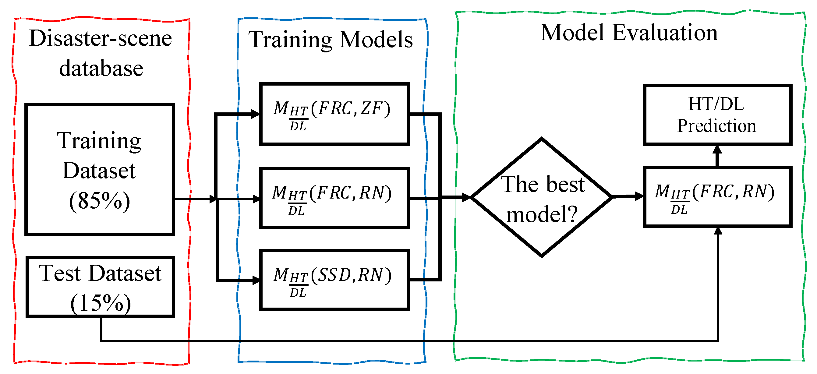
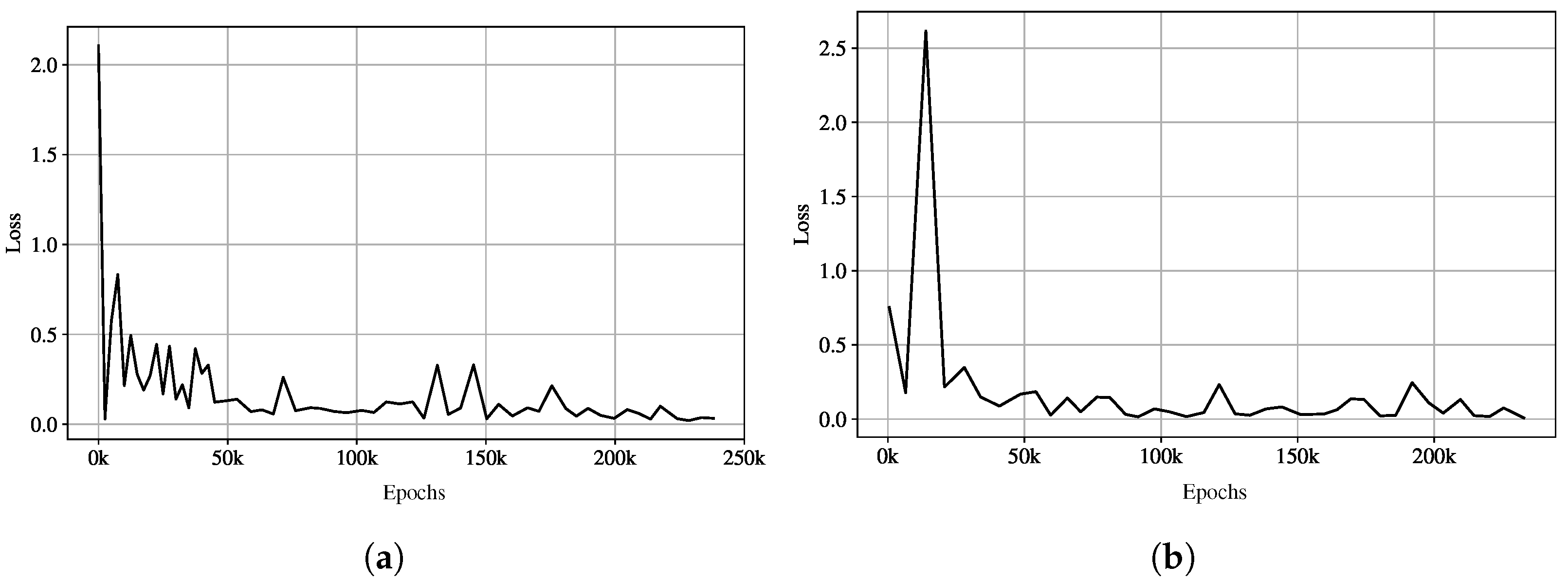
4. Performance Evaluation

With the deep-learning models defined previously, this section aims to conduct experimental testing based on the multi-hazard disaster-scene dataset prepared in this work. Quantitative performance measures and graphical analytics are used for this purpose. It is noted that similar to the conventional treatment in bounding-box-based objection detection, it is the class labels that are evaluated. Bounding boxes are used as a visual reference to exam if proper attention zones are produced.

4.1. Performance Measures

The simplest and basic performance measures are based on the calculation of prediction rates given a set of known class labels and classification labels, resulting in the counting of four prediction consequences, including the number of true-positive (TP), true-negative (TN), false-negative (FN), and false-positive (FP) predictions. With these counts, simple accuracy measures, including the confusion matrix, the Overall Accuracy ($OA$), and the Average Accuracy ($AA$), can be defined. These simple accuracy measures may be misleading in practice, particularly when the learning data is imbalanced. In this work, a comprehensive set of performance metrics, including scalar and graphic metrics, are adopted.

Precision and recall are improved performance measures in the field of information retrieval and statistical classification, also widely used in the deep-learning-based object-detection literature. The precision is the ratio of the number of positive samples to the total number retrieved (defined as $TP/(TN+FP)$). It reflects the ability of a model to predict only the relevant instances. The recall rate refers to the ratio of the number of positive samples retrieved and the number of all truly positive samples in the dataset (defined as $TP/(TP+FN)$. The recall indicates the ability of a model to find all relevant instances. The two measures are coupled; in general, when both measures approach 1, they reflect a more accurate model. However, practical models often achieve higher precision and low recall or vice versa. Based on precision and recall, the $F_1$ score, which is the harmonic mean of precision and recall, quantifies the balanced performance of a classification model.

The precision and recall can be evaluated using a default threshold value (i.e., 0.5) in the classification layer. By varying the underlying classification threshold, a precision-recall curve (PRC) can be plotted. Technically, a maximal F-1 measurement (and the optimal threshold) can be recognized from this PRC curve. Another graphical evaluation approach, called the Receiver Operating Characteristic (ROC) curve, is often used in the literature on machine learning. A ROC is created by plotting the true-positive rate (which is the same as the recall measure) against the false-positive rate, during which the classification threshold varies as well. Given a PRC or ROC associated with an acceptable classification model, one usually observes that as the recall (or the true-positive rate) increases, the precision decreases, and the false-positive rate increases. Last, it is noted that with the ROC curve, the area under the ROC curve ($AUC$) can be used as a lumped measure that indicates the overall capacity of the model. In this paper, the baseline confusion matrices, four performance statistics $AUC$, $F_1$ score, $AA$, and $OA$, and two graphical curves (PRC and ROC curves) are used as performance measures.

4.2. Model Performance

The performance of the predictive models for hazard-type and damage-level classification is evaluated separately in this section. In each case, besides the straightforward confusion matrix, the scalar accuracy measures, including the $F_1$ score, the overall accuracy ($OA$), the average accuracy ($AA$), and the area under the ROC curve ($AUC$) are jointly considered. The graphical ROC and PRC of the best models selected in this paper are further used to examine the model capacity and robustness.

4.2.1. Hazard-Type Prediction Performance

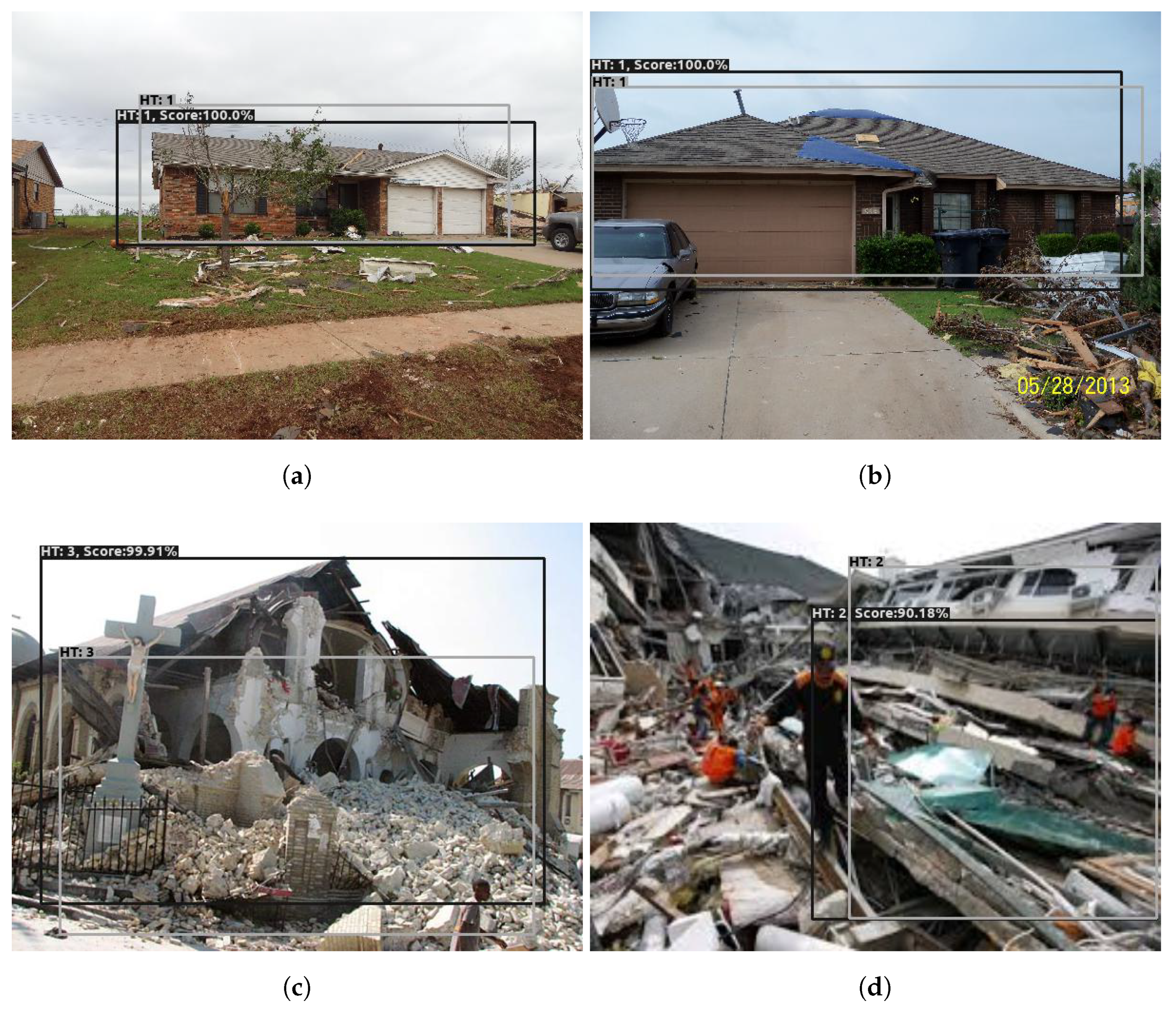
Three hazard-type prediction models are assessed herein (Table 1). Figure 7 demonstrates four sample prediction results from $M_{HT}(FRC,RN)$. In each predicted instance, both ground-truth and predicted information are annotated, including the bounding boxes, the class labels, and the prediction scores. Regarding the bounding-box prediction, first, it is observed that our strategy of emphasizing the spatial boundaries of damaged buildings is largely confirmed. In all cases, the bounding boxes tend to envelop the buildings. It is observed that for tornado scenes, as illustrated in Figure 7a,b, both bounding boxes and hazard-type are more accurately detected. For earthquake and tsunami scenes, instances exist that are challenging to differentiate for human analysts if one inspects Figure 7c,d. Nonetheless, the model largely has learned the salient differences in terms of geometric distinction of debris patterns. In addition, while outlining the bounding box in Figure 7d, it seems that the analyst emphasizes the salient region that can inform the tsunami hazard-type. Therefore, a smaller box is given. In terms of discriminating its damage-level, it is excessively small.

Based on the testing data, the accuracy measurements are reported in two tables.

Table 2. Confusion matrix of hazard-type prediction.

	Prediction	${\mathit{M}}_{\mathit{HT}}(\mathit{FRC},\mathit{ZF})$				${\mathit{M}}_{\mathit{HT}}(\mathit{FRC},\mathit{RN})$				${\mathit{M}}_{\mathit{HT}}(\mathit{SSD},\mathit{RN})$
Actual		Tornado	Tsunami	Earthquake	Total	Tornado	Tsunami	Earthquake	Total	Tornado	Tsunami	Earthquake	Total
Tornado		72	2	1	75	73	0	2	75	33	3	39	75
Tsunami		4	48	16	68	0	59	9	68	16	19	33	68
Earthquake		9	16	86	111	2	12	97	111	17	22	72	111
Total		85	66	103	254	75	71	108	254	66	44	144	254

reports the confusion matrix for each hazard-type model. In

Table 3. Performance of hazard-type prediction.

	${\mathit{M}}_{\mathit{HT}}(\mathit{FRC},\mathit{ZF})$			${\mathit{M}}_{\mathit{HT}}(\mathit{FRC},\mathit{RN})$			${\mathit{M}}_{\mathit{HT}}(\mathit{SSD},\mathit{RN})$
	$\mathit{AUC}$	${\mathit{F}}_1$ Score	$\mathit{AA}$	$\mathit{AUC}$	${\mathit{F}}_1$ Score	$\mathit{AA}$	$\mathit{AUC}$	${\mathit{F}}_1$ Score	$\mathit{AA}$
Tornado	0.98	0.90	0.96	0.99	0.97	0.97	0.64	0.47	0.44
Tsunami	0.83	0.72	0.705	0.92	0.85	0.87	0.57	0.34	0.28
Earthquake	0.86	0.80	0.774	0.91	0.88	0.88	0.55	0.57	0.65
OA	0.81			0.90			0.49

, four accuracy measures are listed, including the AUC based on the ROC curve as a measure of model capacity, the $F_1$ score as the primary accuracy measure, and the $AA$ as a simple accuracy measure. These three measures are calculated as different class labels (the hazard-type of Tornado, Tsunami, and Earthquake). Then the overall accuracy measure, $OA$, is given for each model. The following observations are summarized based on these performance measurements.

First, the high $AUC$ scores of both the FRC-based models signify their higher prediction capacities than the SSD model at all hazard types. In terms of the $F_1$ scores, the FRC-based models again show much greater accuracy than the SSD model. If the $F_1$ scores alone are compared, one may see that when the Resnet-50 is used as the feature extractor, slightly better classification accuracy is observed than the ZF-based model. The $AA$ measure shows a consistent trend as the $F_1$ score. On the other hand, when the SSD model $M_{HT}(SSD,RN)$ is concerned, even with the more competitive feature extractor (ResNet-50), its accuracy drops significantly. Based on this evidence, it is argued that the use of Faster R-CNN as the basis for hazard-type prediction is superior to the SSD-based architecture.

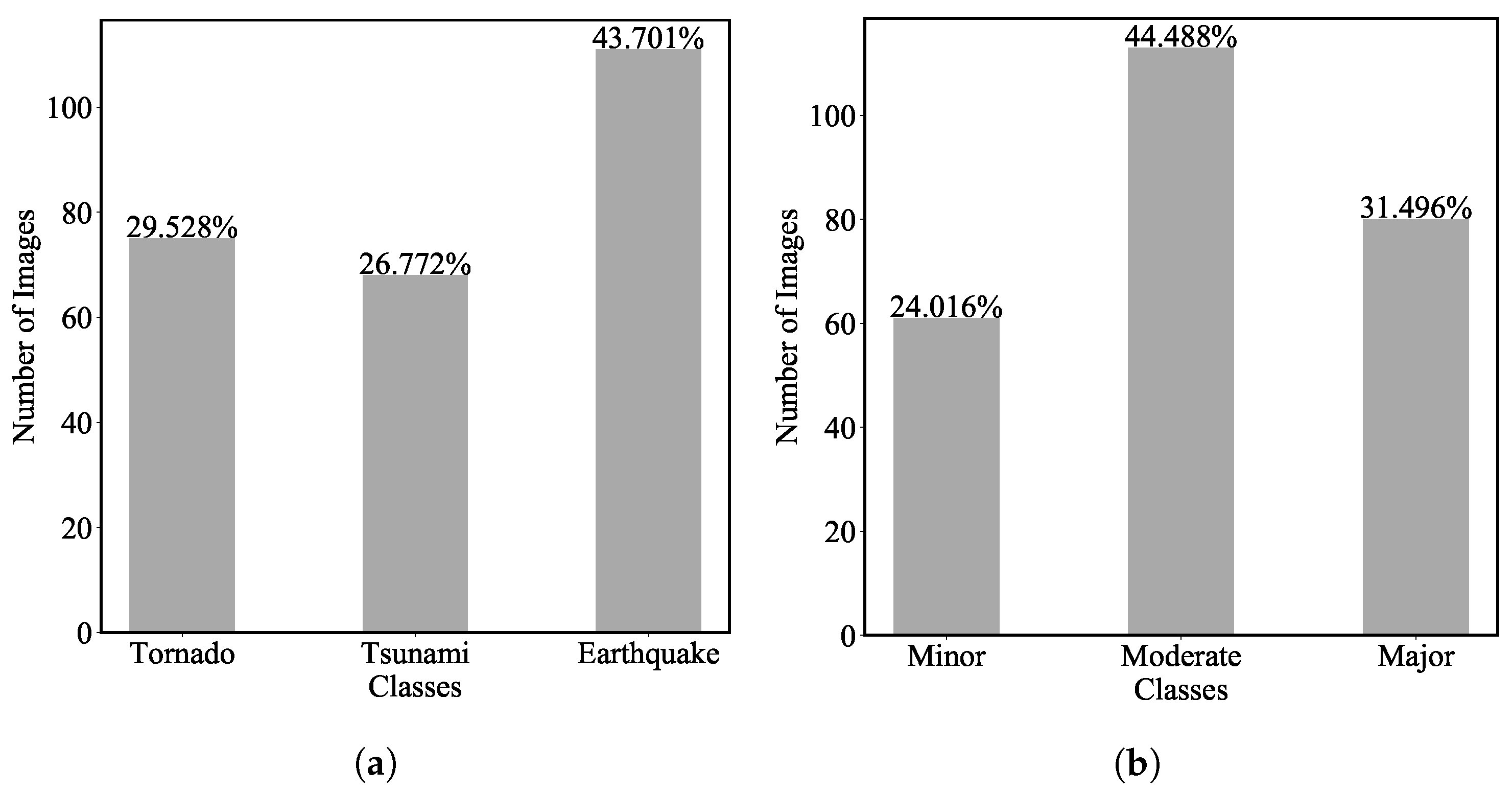
Between the two Faster R-CNN models, $M_{HT}(FRC,ZF)$ and $M_{HT}(FRC,RN)$, it can be seen that this hazard-type detector is more sensitive to the tornado disaster than to the earthquake disaster, and the last is the tsunami disaster. To comprehend this observation, the percentages of images of different hazard types in the learning datasets may provide some insight. It is found that the earthquake images are about 42% of the total samples, tornado images about 25%, and tsunami images around 33%. This indicates that the data is relatively not well-balanced but not severely imbalanced, implying that data imbalance does not sufficiently explain the lowest performance in tsunami disaster prediction. By visually inspecting the images and further reflecting on the strategy of using building-focused bounding boxes when annotating the data, the authors speculate that for a tsunami image, by the mandatory attention of the visual cues on building objects using bounding boxes, this treatment may tend to miss other important visual cues, particularly water. In other words, by confining the visual cues within the bounding boxes for only the buildings, more subjective uncertainties are introduced to discriminate tsunami scenes against the other two.

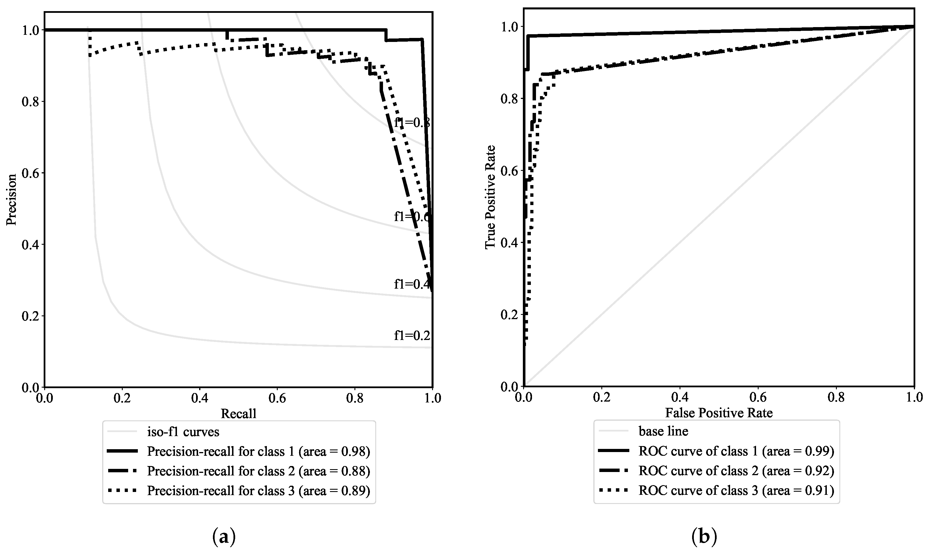
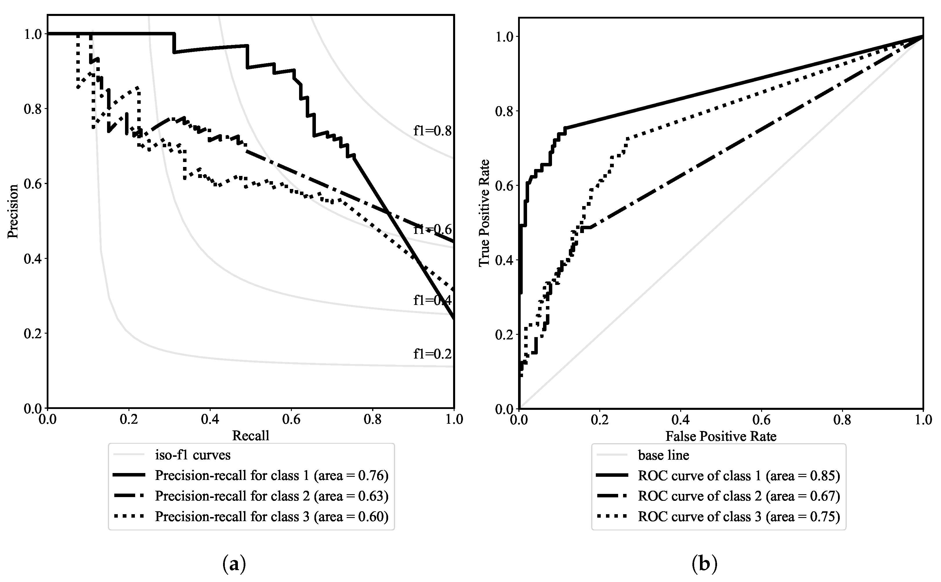
As observed previously, the best model for hazard-type prediction is $M_{HT}(FRC,RN)$. To better assess its capacity and robustness, the PRC and ROC curves are illustrated in Figure 8. In the PRC plot, the iso-contours of the $F_1$ values with various classification thresholds are illustrated, which lead to the $F_1$ contours of 0.2, 0.4, 0.6, and 0.8. The baseline prediction line is marked in the ROC lines, indicating that any ROC above this diagonal line implies a useful classification model. From PRC and ROC plots, which are overall monotonic and symmetrically concave, it is evident that the model consistently has a strong capacity and robustness at most select thresholds.

4.2.2. Damage-Level Prediction Performance

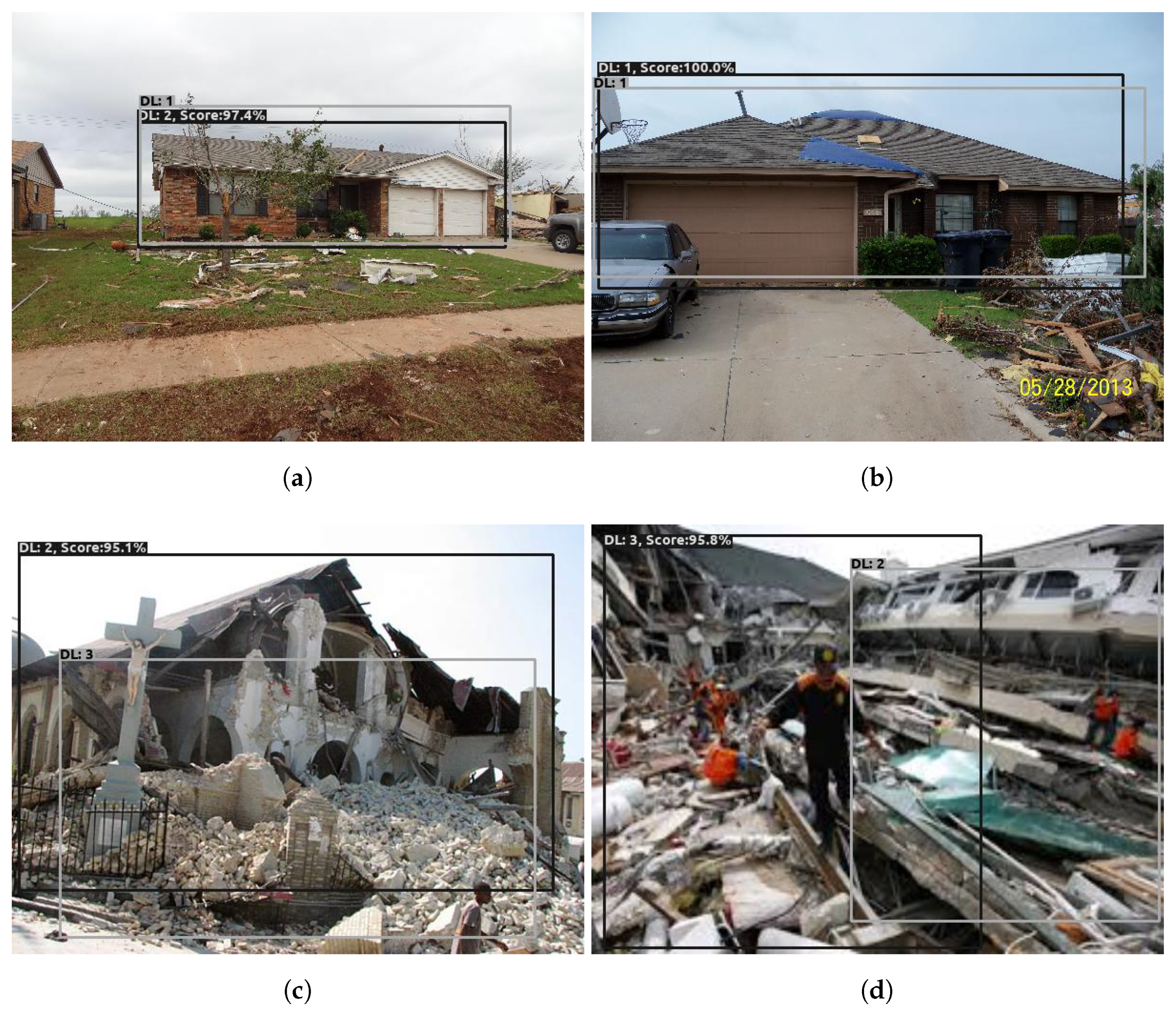
Three damage-level prediction models are assessed herein (Table 1). Figure 9 first demonstrates the damage-level prediction results using the same four sample inputs as in Figure 8 using the damage prediction model $M_{DL}(FRC,RN)$. As shown earlier, the bounding boxes tend to envelop the buildings with different damage features. It is interesting to note that in Figure 9d, the damage prediction model chooses a much different bounding box and reports a correct damage level. In contrast, the underlying bounding-box emphasizes tsunami hazard features, and an erroneous damage level is given as ‘ground-truth’. This implies the subjective variability introduced by human annotators.

The performance measurements are reported in terms of the confusion matrices and scalar measures in

Table 4. Confusion Matrix of damage-level Models.

	Predict	${\mathit{M}}_{\mathit{DL}}(\mathit{FRC},\mathit{ZF})$				${\mathit{M}}_{\mathit{DL}}(\mathit{FRC},\mathit{RN})$				${\mathit{M}}_{\mathit{DL}}(\mathit{SSD},\mathit{RN})$
Actual		Minor	Moderate	Major	Total	Minor	Moderate	Major	Total	Minor	Moderate	Major	Total
Minor		27	24	10	61	46	7	8	61	29	8	24	61
Moderate		23	57	33	113	19	55	39	113	24	21	68	113
Major		10	34	36	80	4	18	58	80	13	15	52	80
Total		60	115	79	254	69	80	105	254	66	44	144	254

and

Table 5. Performance of damage-level classification.

	${\mathit{M}}_{\mathit{DL}}(\mathit{FRC},\mathit{ZF})$			${\mathit{M}}_{\mathit{DL}}(\mathit{FRC},\mathit{RN})$			${\mathit{M}}_{\mathit{DL}}(\mathit{SSD},\mathit{RN})$
	$\mathit{AUC}$	${\mathit{F}}_1$ Score	$\mathit{AA}$	$\mathit{AUC}$	${\mathit{F}}_1$ Score	$\mathit{AA}$	$\mathit{AUC}$	${\mathit{F}}_1$ Score	$\mathit{AA}$
Minor	0.59	0.44	0.44	0.85	0.71	0.75	0.55	0.46	0.47.5
Moderate	0.50	0.50	0.50	0.67	0.57	0.49	0.51	0.27	0.18.58
Major	0.58	0.45	0.45	0.75	0.62	0.72	0.60	0.46	0.65
OA	0.47			0.63			0.50

, respectively. The most significant observation is that damage-level prediction performance decreases considerably compared to the hazard-type prediction over the testing data. In terms of both the $AUC$, $F_1$ score, the $AA$’s, and $OA$’s, none of the performance measurement exceeds 0.9. Nonetheless, the model with the highest performance values is found in $M_{DL}(FRC,RN)$, which shows moderate performance with an overall accuracy of 62.6% and $AUC$ and $F_1$ scores both greater than 0.5 at all damage-level predictions, albeit an alarming accuracy at predicting moderate-level damage. The two other damage-level prediction models, $M_{DL}(FRC,ZF)$ and $M_{DL}(SSD,RN)$, manifest unsatisfactory prediction performance. This implies that the ‘strong’ Faster R-CNN model with a ‘moderate’ ZF feature extractor or the ‘normal’ SSD model with a ‘strong’ Resnet feature extractor cannot sufficiently discriminate damage-level as human experts can do. The model $M_{DL}(FRC,RN)$ with a strong feature extractor and a strong region-proposal model can correctly detect damage-level. If one scrutinizes all the model performance measurements, even with two non-satisfactory models, it is evident that predicting moderate-level damage poses to be the most challenging one. This aspect, as well as the overall moderate performance, is further discussed later.

The ROC and PRC plots in Figure 10 further illustrate the moderate predictive capacity of the model $M_{DL}(FRC,RN)$. Compared to the ROC and PRC plots for the best hazard-type model $M_{HT}(FRC,RN)$, it is seen that both predictive capacity and robustness degrade. Moreover, both graphical analytics show a relatively high capacity to predict minor-damaged buildings, moderate in major-damage prediction, and less satisfactory in minor-damage prediction at all possible variable classification thresholds.

4.3. Observation

The primary observations from the experiments above are multi-fold, which are listed below:

• Hazard-type detection achieves statistically high performance over hazard-type (very high accuracy on tornado-wind scenes, high on the earthquake scene, and weak on the Tsunami-wave scene), and the best model architecture is $M_{HL}(FRC,RN)$.
• Damage-level prediction retains moderate yet explainable performance; nonetheless, the model $M_{DL}(FRC,RN)$ secures acceptable performance on minor- and detecting major-damage level.
• The bounding-box-based detection is overall satisfactory and sufficiently captures the attention zones in disaster-scene images.
• Regarding the three-model architecture for the two disaster-scene understanding tasks, it is observed too that Faster R-CNN as a general object-detection architecture with outputs of both bounding boxes and class labels has a superior performance.

More explanations and limitations in the proposed methodology framework are discussed in the following.

5. Discussion

5.1. Justification of Accuracy

First, to enlighten the discussion regarding the accuracy of image-based damage classification, the authors retrieve relevant accuracy results from the literature. It is noted that again there are no similar efforts that use mobile RS images. Ref. [43] reviewed many efforts, where categorical structural damage was classified using traditional RS images. First, the average or overall accuracy ranged from 70% to 90%, depending on the availability and quality of the data; higher rates were usually a result of possessing high-quality pre- and post-event data. Ref. [44] conducted damage classification using synthetic aperture radar (SAR) images before and after the 2011 Tohoku Earthquake and Tsunami in Japan. With a traditional machine-learning framework, they reported an average accuracy of 71.1% using the F-1 score. Ref. [45] proposed a deep-learning-based damage detection workflow using the same type of data over the tsunami-related damage as in [44]. They reported a damage-level recognition accuracy of 74.8% over three damaging classes. Ref. [46] identified the significance of fusing the Digital Elevation Model (DEM) with SAR data for damage mapping. In terms of four levels of building damage for an Indonesia tsunami, they reported a higher overall accuracy (>90%) yet a low average accuracy (around 67%). Given such comparison, the authors of this paper argue that towards an image-based classification of structural damage for built objects, an OA measurement of $62.6\%$) as reported by the model $M_{DL}(FRC,RN)$ is not surprisingly low.

To further explain this, three vital differences between traditional RS images and mobile RS images are argued below, which render mobile RS-based damage detection more challenging.

• Bitemporal GIS-ready RT images vs. non-structured mobile images. In traditional RT images, the bitemporal pairs are usually both ortho-rectified and co-registered; therefore, bitemporal pixels for the same objects may only subject to misalignment of a few pixels, which significantly constrains the degree of errors. In the case of mobile images, there are no bitemporal pairs, and the damage is opportunistically captured from an arbitrary perspective of a built object. This difference leads to overall much more uncertainties in mobile RS images towards damage interpretation.
• Bounded vs. unbounded scene complexity. In traditional RT images, most multi-story building objects in the nadir or off-nadir views only show the roof level damage with minimal building elevation coverage. This implies that the structural characteristics are primarily in terms of lines, edges, and corners at the roofs of buildings, which are low-level visual features. When damage occurs, these low-level features are distorted or modified. In mobile images, however, the scene complexity is mounted dramatically, and the involved features are at a high-level, including parts of objects, adjacent objects, and potential relations between adjacent parts or objects.
• Hazard specific vs. hazard-agnostic damage-level. In most RT-based damage-level classification, the hazard-type comes from a single event, and the damage for built objects is extracted from bitemporal images. In this work, treating the damage-level agnostic to hazard-type leads to significant intra-class variations, which are much less significant when using traditional RS images.

Secondly, it is explainable that hazard-type prediction models perform better than the damage-level models in this work. For this performance disparity, three empirical reasons are speculated herein. First, visual clues that imply hazard-type in disaster-scene images are more abundant and distinct than those possibly exploitable for discriminating damage-level. Second, the damage-level semantically imply an increasing order of damage severity. This renders secondary yet significant overlapping in the underlying decision boundaries in the high-dimensional feature space, namely inter-class variations. Third, treating the damage-level not specific but agnostic to hazard-type leads to significant intra-class variations. These three conjunct reasons are believed to corroborate that generic damage-level are much more challenging to learn than hazard types given the same disaster-scene database.

5.2. Suggestions for Future Research

Tornado-scene images in this work should be augmented to include more complexity. It is noticed that when predicting the tornado scenes, very high accuracy is achieved (with an $AA$ up to 0.973 and an $F_1$ score of 0.970; Table 2). The prediction accuracy is high on earthquake-scene prediction ($AA$ = 0.873; $F_1$ score = 0.994); then the least on tsunami-scene ($AA$ = 0.867; $F_1$ score = 0.849). This ranked trend in prediction accuracy essentially coincides with the scene complexity, from low to high: Tornado-wind, Tsunami-wave, and Earthquake-shaking scenes. Essentially, although the disaster-scene database created in this work contains images for events around the world, they are still limited in terms of diversity. Specifically, the tornado-scene images came from a single event and were taken within residential areas from one town (Moore, Oklahoma). Regardless of the relative complexity, nearly all buildings in images are residences captured from their front view. More diversity is in the earthquake scenes from urban settings of two quite different countries, Haiti and New Zealand. Similarly, the tsunami images came from two countries as well, coastal towns in Japan and Indonesia. These distinctions in imagery-scene complexity in terms of their sources and characteristics explain the observed performance. It is suggested that a different source for tornado-scene images may be included to augment the scene complexity.

More flexible bounding-box-based annotations may be designed for very complex disaster-scene images. When the tsunami-wave scene is classified, relatively lower performance is observed with all the three models used. The authors speculate that by annotating bounding boxes and focusing on building objects, the tsunami-specific visual cues, particularly flood-borne debris, tend to be missed by the bounding boxes. The authors argue that this can reduce prediction performance about the tsunami scenes. As observed in Figure 7d and Figure 9d, bounding boxes are predicted differently from the human annotation. This is inevitably due to arbitrary and subjective variations in a subjective human-based process. The models learn the most plausible bounding box statistically in this tsunami-scene image. For damage-level prediction, however, the model chooses the bounding box with the damage-level of the maximum score value, and a much different box is predicted yet with a correct prediction (relative to the mislabeled label by a human analyst). This implies the disadvantage of the proposed simplified annotation process for the human analyst in this work. It is suggested that for very complex disaster scenes, such as hydraulic hazards induced disasters (e.g., flooding, tsunami, and storm surges), multiple and different bounding boxes can be used for characterizing the hazard-type and building damage. This treatment is left for future research.

Hierarchical and fine-grained semantic labeling should be pursued in future research. Related to hazard types, a hierarchical scheme may be designed based on event type; for example, for an earthquake-event scene, the hazard labels may include: shaking, land sliding, liquefaction, ground sinking; whereas related to disaster types, specific damage types may be classified according to element types and location; for example, for buildings, these may include structural beam, wall, or foundation damage and nonstructural-element damage. Nonetheless, this fine-grained labeling demands a much larger-scale database and a more sophisticated model.

Data imbalance in disaster-scene images is intrinsic. First, it is due to the nature of hazards in their frequency; for instance, the returning period of a strong earthquake is much more extended than a windstorm. Second, after an intense event, crowdsourced images from the general public are more focused on severely damaged buildings due to physiological preferences. In recent years, innovative loss functions were proposed that deal with dense objects in images with a high ratio between the foreground objects and background objects [47]. However, in this work, the imbalance occurs within different built objects, which are mainly in the foreground. Future research is needed, and the work of [47] provides an inspiring direction by tuning the loss function.

5.3. Understanding UAV Images

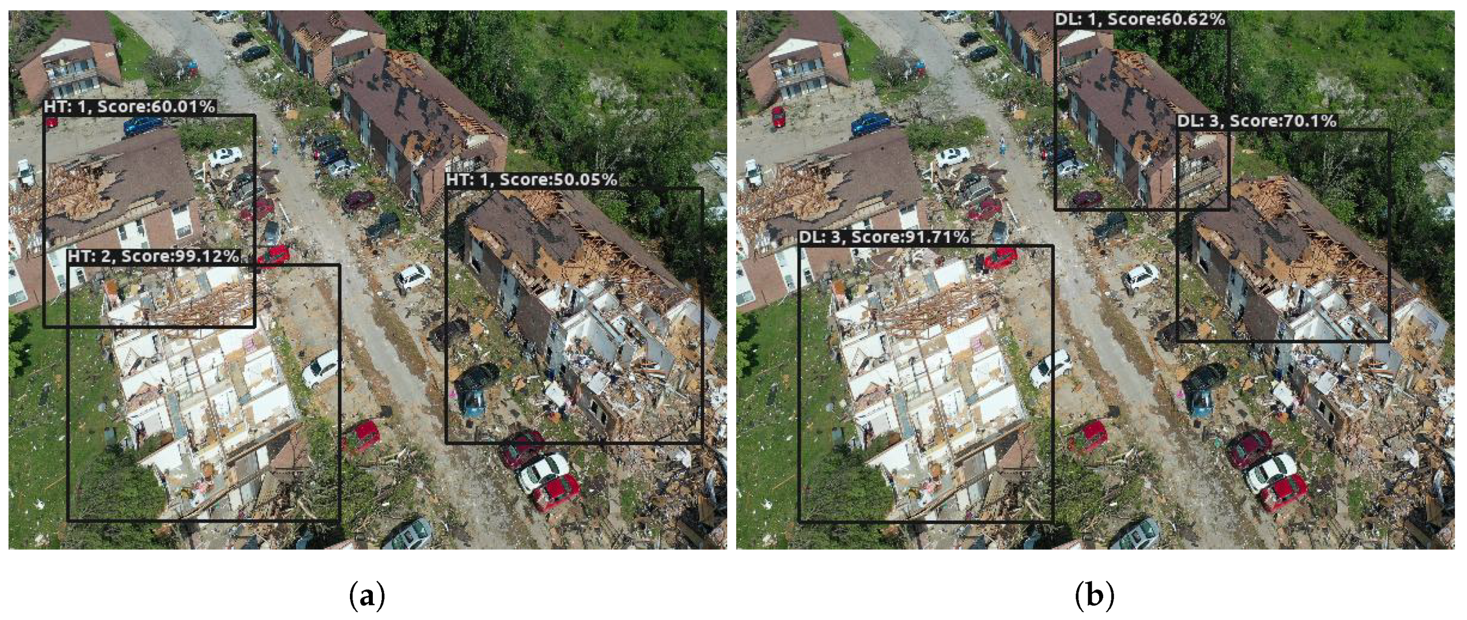
It is asserted in this paper that UAVs are becoming a personal RT platform and a standard tool in professional disaster reconnaissance activities in recent years. In practice, UAVs-based RS images possess special characteristics due to their much flexible imaging geometrics. In general, UAV images according to their coverage and imaging heights can be categorized into three types: (T1) elevation view of buildings if the imaging UAV captures at an AGL height comparable to building heights; (T2) overhead view of one or several buildings when the AGL heights are higher than buildings; (T3), aerial view of a large number of buildings when the AGL is much high (e.g., hundreds of feet above ground). In general, the authors state that the developed models in this work should work well for UAV images from the first category (T1) as they are similar to any ground-level mobile images. For images in T2, the images may still be similar to the mobile images in this paper as one may capture images at a higher ground than buildings. For T3, they should be processed first using photogrammetric methods used for traditional RS images.

In this effort, the models $M_{HT}(FRC,RN)$ and $M_{DL}(FRC,RN)$ developed previously are applied to some sample UAV images, which were captured from a recent tornado disaster reconnaissance (Jefferson City, Missouri). The images were shot at a low altitude over an apartment complex. As shown in Figure 11a, two of three damaged buildings are classified correctly as the tornado hazard-type. The lower left one is classified as the tsunami type because its roof is disappeared, which is a scene not appeared in the tornado-scene images in this paper (that were captured mostly with the front view). For damage-level classification, three buildings are detected in Figure 11b; the predicted damage-level conform to the hazard-agnostic damage classification. This extrapolation effort demonstrates that UAV images may deserve some specific processing to improve accuracy. One possible solution is to exploit the 3-dimensional (3D) embeddings hidden in many overlapped UAV images hence a 3D reconstruction of the scene can be obtained [8,48]. With 3D image-based learning, more granular and representative features may positively augment the model accuracy.

6. Conclusions

In this work, the authors explore the feasibility of a quantitative understanding of disaster scenes from mobile images. To deal with the significant complexity and uncertainties in disaster-scene images, this paper proposes adopting advanced deep-learning models to identify both hazard-type and damage-level embedded in images.

The authors develop three deep-learning models for two disaster-scene understanding tasks: hazard-type identification and damage-level estimation. The following conclusions are resolved by assessing the performance of the two tasks based on quantitative performance measures. First, the performance of the models demonstrates that disaster scenes in mobile RS practice can be modeled, and predictive models with acceptable performance are feasible. Second, it is concluded that hazard-type can be identified with high accuracy due to the underlying abundant visual characteristics. On the other hand, relatively modest performance is observed when the models predict damage level. Empirical explanations are provided, including that the proposed damage-level scaling is agnostic to hazard types and possesses much inter- and intra-class variations. Last, it is observed that the Faster R-CNN architecture with a Resnet-50 CNN as the feature extract excels with the highest performance in this effort.

With these conclusions, the authors expect that higher-performance predictive models for disaster-scene learning can be developed by enhancing data volume, veracity, and better-suited deep-learning architectures. The proposed concept of mobile imaging-based disaster-scene understanding and the developed frameworks in this paper can facilitate the automation of imaging activities conducted by either professionals or the general public as smart and mobile devices become ubiquitous, enabling data-driven resilience of disaster response.