An Advanced Spectral–Spatial Classification Framework for Hyperspectral Imagery Based on DeepLab v3+

Abstract

DeepLab v3+ neural network shows excellent performance in semantic segmentation. In this paper, we proposed a segmentation framework based on DeepLab v3+ neural network and applied it to the problem of hyperspectral imagery classification (HSIC). The dimensionality reduction of the hyperspectral image is performed using principal component analysis (PCA). DeepLab v3+ is used to extract spatial features, and those are fused with spectral features. A support vector machine (SVM) classifier is used for fitting and classification. Experimental results show that the framework proposed in this paper outperforms most traditional machine learning algorithms and deep-learning algorithms in hyperspectral imagery classification tasks.

1. Introduction

With the development of remote sensing technology in the late 20th century, the emergence of hyperspectral imagery (HSI) technology has attracted widespread attention in various fields. Unlike natural images and multispectral images, the resolution of hyperspectral images in the spectral range is very high, generally in the order of 10⁻²λ. A hyperspectral imager can record hundreds of channels of spectral band information from ultraviolet to midinfrared. This rich spectral band information has become the focus of many fields such as land monitoring, crop growth, petroleum exploration, and military target recognition.

Hyperspectral imagery classification (HSIC) is more difficult than natural image classification for two primary reasons [1]:

(a)

The spectral bands of hyperspectral images have high dimensionality, which increases the computational complexity. Moreover, according to the Hughes phenomenon, as the dimension number increases, the classification accuracy first increases and then decreases.

(b)

The spatial resolution of hyperspectral images is very low, and one pixel typically represents a distance of tens of meters. Therefore, the number of pictures in each dataset is very small, and extracting spatial features is more difficult.

At present, there are several different ideas to solve the problem of excessive dimensionality of hyperspectral datasets. First, the dimensionality of the spectral band can be reduced using one of the two broad strategies: projection and manifold learning. Principal component analysis [2] is a typical linear dimensionality reduction method in projection. The purpose is to map high-dimensional data to a low-dimensional space through a certain linear projection. In some high-dimensional images with more noise, the effect of principal component analysis is not satisfactory. Specifically, when the variance of the noise contained in a principal component with a large amount of information is greater than the variance of the signal, the quality of the image formed by the principal component is poor. Green [3] et al. addressed this problem using the MNF (minimum noise fraction) rotation. It essentially includes two stacked principal component transformations. When faced with some manifold data such as Swiss rolls, projection-based dimensionality reduction methods cannot solve the problem well; therefore, manifold learning is a better choice. The main methods are Isomap algorithm [4], Laplacian eigenmaps [5], and so on. In addition to dimensionality reduction methods, 3D-CNN in deep learning has also been applied to hyperspectral datasets. Chen [6] and Ying [7] used 3D-CNN to directly extract advanced features in hyperspectral images and realized the classification of hyperspectral images, cleverly avoiding the high dimensionality of hyperspectral images. However, the computational complexity of 3D-CNN is relatively large, and the training time of neural networks using 3D-CNN is relatively long.

To fully extract the effective feature information in the hyperspectral image, people try to combine different methods to think about the features in the spectral domain and spatial domain. In traditional machine-learning methods, some typical classifiers, such as k-nearest neighbors [8], support vector machines [9,10], etc., used the characteristic information of the spectral domain as the division standard and adopted different methods to effectively classify hyperspectral images. The powerful feature extraction ability makes deep learning attractive for traditional optical problems [11,12,13] and hyperspectral classification problems. Stacked AutoEncoders (SAE) [14] used the fusion feature information of the spectral domain and the spatial domain as training features for the classification of hyperspectral images. This is the first time that deep learning has been applied to the classification of hyperspectral images. Convolutional neural network (CNN) has local perception and parameter sharing and can learn different levels of spatial feature information. This weight-sharing network structure reduces the complexity of the network model, reduces the number of weights, and can effectively learn the corresponding features, while avoiding the complex feature extraction process. However, continuous convolution and pooling operations in the network destroy the original spatial information and reduce the resolution, which decreases the classification accuracy of picture. The fully convolutional network (FCN) [15] converts the fully connected layer at the end of the convolutional neural network into a convolutional layer. This makes it possible for the convolutional neural network to achieve pixel-level classification. Combining fully convolutional neural network and ELM (extreme learning machine) [16] has achieved the pixel-level classification of hyperspectral images.

We propose a classification structure based on the DeepLab v3+ network for the problem of how to use the limited hyperspectral image data to fully mine the feature information, thereby improving the accuracy of hyperspectral image classification. The main contributions of this article are summarized as follows:

(1)

We utilize DeepLab v3+ as the neural network structure to extract spatial domain features and merge them with spectral domain features. DeepLab v3+ is one of the fourth-generation DeepLab series of semantic segmentation networks developed by Google and has the best comprehensive performance so far. We are the first to apply the latest version of the DeepLab network to the hyperspectral image classification task.

(2)

We use the PCA method to reduce the dimensionality of the original hyperspectral image. In the spatial feature extraction stage, we select the first three principal components and the first principal component as training data and labels [16] to solve the dimensionality problem of the hyperspectral imagery.

(3)

We select different classifiers such as SVM, KNN, etc., to complete the task of hyperspectral image classification. We test and compare the classification accuracy under different conditions.

2. DeepLab v3+ and Proposed Framework

2.1. DeepLab v3+

DeepLab v3+ [17] is the latest work in the DeepLab series neural networks of semantic segmentation. Its predecessors include DeepLab v1, v2, and v3. The DeepLab series of neural networks use deep convolutional neural networks (DCNNs), which have excellent translation invariance so that they have good image-level classification capabilities. However, it is difficult for DCNNs to deal with the pixel-level classification problem, which is also an urgent problem for semantic segmentation. Therefore, in light of the following main problems, the author [17] has proposed solutions in different versions of DeepLab.

Continuous convolution and pooling in DCNNs inevitably lead to a decrease in the resolution of feature maps, which affects the final segmentation accuracy. Inspired by the paper [18], the author of DeepLab used the atrous convolution in the v2 version. The mathematical reasoning process of the hole convolution is described in detail [18] elsewhere; we discuss it briefly. Figure 1 represents the comparison of convolution principles in two different ways.

Let $F:Z^2\to R$ be a discrete function, and ${\mathsf{\Omega }}_r={\left[-r,r\right]}^2\cap Z^2 (r>0)$. Let the convolution kernel be $k:{\mathsf{\Omega }}_r\to R$, then the size of the convolution kernel is (2r + 1)². The definition of discrete convolution $\ast$ can be obtained from the above conditions:

$$\left(F\ast k\right)\left(p\right)={\sum }_{s+t=p}F\left(s\right)k\left(t\right)$$

(1)

when considering the atrous convolution, let $l$ be the hole coefficient. The atrous convolution ${\ast }_l$ with the atrous coefficient $l$ can be defined as:

$$\left(F{\ast }_{l}k\right)\left(p\right)={\sum }_{s+lt=p}F\left(s\right)k\left(t\right)$$

(2)

Secondly, another major problem with DCNNs is that due to the fixed parameters of the fully connected layer at the end of the network, the input images need to have a fixed size. The usual solution is to crop or scale the input image. However, in the process of cropping and scaling, the target object in the picture is deformed, resulting in a decrease in recognition accuracy. To address this problem, atrous spatial pyramid pooling (ASPP) is added to the DeepLab series neural network combining the design ideas of atrous convolution and spatial pyramid pooling (SPP) [19], which are represented in Figure 2.

The spatial pyramid pooling structure is generally placed before the last fully connected layer of the network. When the feature map of the size $\left(w,h\right)$ output by the previous layer is passed into the SPP, it is divided multiple times. The same image is divided into $m\times n$ image blocks of size $\left(w/m,h/n\right)$ by the division scale $\left(m,n\right)$. Each image block in each divided image is put into the pooling layer separately and finally linked to a fully connected layer after joining. The biggest advantage of the structure is that it solves the size problem of the input picture. Due to the flexibility of the input size, the network can extract the convergence features under different pooling window sizes to improve the classification accuracy. Similarly, each feature map is separately convolved by convolution kernels with different dilation rates and then concatenated together in an atrous spatial pyramid pooling structure.

In the v3+ version, in order to integrate multiscale information, the v3 network is designed as an Encoder, and then the spatial resolution is restored in the Decoder structure. The Encoder–Decoder model is commonly used in semantic segmentation. During the test, DeepLab v3+ showed good segmentation performance. In the PASAL VOC 2012 dataset, it produced an mIOU index of 89.0, which is the best performance so far. Therefore, we choose DeepLab v3+ as the main network for feature extraction in our research. Figure 3a shows the network structure of DeepLab v3+.

2.2. Proposed Framework

Figure 3b shows the framework we proposed of hyperspectral image classification. The framework can be roughly divided into three parts: PCA dimensionality reduction, feature extraction and fusion, and the use of classifiers to achieve pixel-level classification. The specific details and mathematical principles of the framework are as follows.

The unprocessed hyperspectral image is regarded as a series of samples. Assume that the matrix size represented by the hyperspectral image is $h\times w\times n$, where $h\times w$ represents the resolution of the image and $n$ represents the number of spectral channels. If $x_i\in R^n$ is represented by a column vector, then the dimensionality reduction goal is to reduce the dimensionality of $X\in R^{n\times h\times w}$ composed of $h\times w$ samples to $\widehat{X}\in R^{k\times h\times w}\left(k\le n\right)$. The process of principal component analysis is as follows.

Let $u_i$ be the $i-th$ principal component. The optimization is:

$$\underset{u_i}{\mathrm{argmax}}({\sum }_{j=1}^n\left|proj\left(x_j,u_i\right)\right|), \left(x_j,u_i\in R^n\right)$$

(3)

and the projection length of $x_j$ on $u_i$:

$$proj\left(x_j,u_i\right)=\frac{x_j\cdot u_i}{||u_i||{}^2}=\frac{x_j{}^T{u}_i}{||u_i||{}^2}$$

(4)

Let $||u_i||=1$, and we already know $X=\left[x_1,x_2,\cdots ,x_{h\times w}\right]$. Hence, it can be shown:

$$({\sum }_{j=1}^n\left|proj\left(x_j,u_i\right)\right|)=\underset{u_i}{\mathrm{argmax}}\left(u_i{}^{T}X{X}^T{u}_i\right)$$

(5)

The matrix $X{X}^T\in R^{n\times n}$ is positive definite. Therefore, $u_i{}^{T}X{X}^T{u}_i$ is positive definite quadratic form, and it has a maximum value. Under the constraint of $u_i{}^T{u}_i=1$, we obtain $X{X}^T{u}_i=\alpha u_i$ by Lagrange multiplier method. α is the eigenvalue of the matrix $X{X}^T$, and the objective function takes the maximum value when $u_i$ takes the eigenvector corresponding to α. We can get:

$$\underset{u_i}{\mathrm{argmax}}\left(u_i{}^{T}X{X}^T{u}_i\right)=\alpha u_i{}^T{u}_i=\alpha$$

(6)

where $u_i$ is the $i-th$ principal component. Taking the eigenvectors of the first k eigenvalues and the corresponding matrix, $U=\left[u_1,u_2,\cdots ,u_k\right]\in R^{n\times k}$. Finally, a dataset reduced from n dimensions to k dimensions can be obtained by

$$\widehat{X}=U^{T}X\in R^{k\times h\times w}$$

(7)

Using an established method [16], the dimensionality of original hyperspectral dataset is reduced by PCA. As a method of dimensionality reduction, PCA only reduces the dimensionality of the data while there is very little information loss. The introduction of PCA is to avoid the use of three-dimensional convolution in the feature extraction process which is computationally intensive. If we do not use PCA, three-dimensional convolution has to be used in all data, including training set and test set generally. Therefore, the introduction of PCA theoretically does not lead to biased results.

We take the first three principal components, namely $k=3$, as the dataset, and take the first principal component, namely $k=1$, as the label. All data processed by PCA are converted into uint8 format; therefore, in theory, they are all integers in the range of $\left[0,255\right]$. The main reason for using the first principal component as the label is that the data after dimensionality reduction remove the redundant information in the spectral domain and only a single channel is retained. The process retains the feature relationship of the object represented by each pixel in space, which is also an essential element for extracting spatial features.

To expand the number of samples so as to extract the spatial feature information abundantly, we use an established method [20] to crop the reduced-dimensional images and labels. The size of the cropping window is $45\times 45$ pixels, the stride is 5 pixels, and the pictures and labels are cropped from left to right and top to bottom. Then, the cropped pictures and corresponding labels are used as the training set.

In the spatial feature extraction stage, we choose resnet50 as the backbone of DeepLab v3+ and set the label number to 256. The crossentropy loss function is the optimization target, as follows:

$$H\left(p,q\right)=-{\sum }_{i=1}^{n}p\left(x_i\right)log\left(q\left(x_i\right)\right)$$

(8)

where $p$ is the expected output and $q$ is the actual result. Crossentropy is used to evaluate the difference between the current training probability distribution and the true distribution. Therefore, it is reasonable to reduce the loss function so that the probability distribution of the actual output and the probability distribution of the expected output are as close as possible. Other related training parameters are given in

Table 1. Training parameters in DeepLab v3+.

Output stride	16
Learning rate	0.001
Learning rate scheduler policy	Poly
Weight decay	0.0001

.

After the DeepLab v3+ network is trained, the dimensionality-reduced and not cropped picture with the size of $W\times H\times 3$ is input into the network, and the spatial feature with the size of $W\times H\times 256$ can be obtained without resolution loss. The pixel matrix with the size of $W\times H\times K$ without dimensionality reduction is considered as a spectral domain feature and fused with spatial features. Since the ultimate purpose is to classify each pixel, it is necessary to fuse the spatial and spectral features of each pixel. The number of pixels in the picture is $W\times H$. After normalizing the spatial and spectral features, respectively, the two features are stitched and integrated in the third dimension to complete the feature fusion process. In addition, the size of fusion feature is $W\times H\times \left(256+K\right)$. Finally, we select different classifiers, such as SVM, KNN, etc., and input the fusion features into the classifier for fitting and comparing.

In terms of evaluation, hyperspectral imagery classification generally uses overall accuracy (OA), average accuracy (AA), and κ coefficients, which are all calculated based on the confusion matrix. Among them, OA refers to the ratio of the number of correctly classified category pixels to the total number of pixels, AA refers to the average value of the recall of each category, and κ coefficient is an indicator of consistency.

3. Experimental Results

We selected three hyperspectral datasets: Pavia University [21], Kennedy Space Center [22], and HyRANK [23]. These hyperspectral datasets are public and open source. Pavia University is part of the hyperspectral data imaged in 2003 in the Italian city of Pavia. The size of the hyperspectral image is 610 × 340 pixels, with a total of 115 bands. After removing water vapor noise, there are 103 bands, in the wavelength range of 0.43–0.86 μm. The data contain nine types of labels, a total of 42,776 pixels. The Kennedy Space Center dataset was captured by the AVIRIS sensor on 23 March 1996. It contains 176 spectral bands after removing water vapor noise and 13 types of labels. The HyRANK dataset was acquired by the Hyperion sensor, and each image has 176 spectral bands. To test the generalizability of this feature extraction framework, two pictures with real labels in the dataset, Loukia and Dioni, were selected. The former includes 14 types of labels, and the latter includes 12 types of them. We randomly selected 5% of the pixels of each category in Pavia University and Kennedy Space Center, and 10% in HyRANK as training set, and used the rest as the test set.

Each pixel in the hyperspectral remote sensing image represents a ground distance from about tens to hundreds of meters. In other words, each pixel can be regarded as a sample, and an image contains tens of thousands of such samples. Each sample contains the information of spectral band, and there is also a spatial dimension relationship between them. Therefore, the data of hyperspectral image are sufficient.

The influence of different classifiers and feature types on the classification results are verified separately by controlling variables. In this process, we use the Pavia University dataset and the Kennedy Space Center dataset and compare the experimental results with other literature. To verify whether the proposed framework is equally effective for the new dataset in the feature extraction stage, we use the image Loukia in the HyRANK dataset as training set of DeepLab v3+ and the image Dioni as test set.

3.1. Comparison Between Different Classifiers

In this study, five machine learning classifiers, KNN, logistic regression, decision tree, naive Bayesian model, and SVM were selected, and the established classification algorithms [14,16], such as SRC-T (SRC classifier with diagonal weight matrix T), ELM, SVM-RBF (SVM classifier with radial basis function), SAE-LR (stacked AutoEncoders with logistic regression), and CNN, were compared with our framework.

Table 2. Classification accuracy (%) for the Pavia university dataset via different classifiers we used in this paper.

CLASS	KNN	Logistic Regression	Decision Tree	Naive Bayesian Model	SVM
1	98.72	93.79	92.16	96.17	99.19
2	97.81	98.34	94.98	98.04	99.48
3	96.69	97.05	84.67	85.92	99.30
4	98.57	97.07	81.25	47.66	97.53
5	98.00	99.92	93.48	84.52	99.92
6	99.39	98.43	92.06	86.60	99.79
7	96.63	90.20	84.68	77.17	98.90
8	98.01	89.37	82.19	78.53	96.91
9	100.00	98.04	99.22	100.00	99.78
OA	98.16	96.51	91.49	85.33	99.10
AA	98.20	95.80	89.64	83.85	98.98
Kappa	97.56	95.36	88.73	81.40	98.81

and

Table 3. Classification accuracy (%) for the Kennedy Space Center dataset via different classifiers we used in this paper.

CLASS	KNN	Logistic Regression	Decision Tree	Naive Bayesian Model	SVM
1	93.89	96.65	86.07	93.47	98.89
2	80.07	98.65	48.60	86.59	100
3	98.12	100	76.50	95.24	97.98
4	97.02	100	52.36	80.75	99.13
5	99.32	100	45.18	96.58	96.20
6	100	100	52.97	99.43	100
7	100	93.46	40.13	100	100
8	99.74	98.02	87.88	67.10	91.42
9	96.30	99.80	84.31	78.97	100
10	99.72	100	69.65	99.68	99.47
11	95.38	94.75	93.16	96.21	98.74
12	98.09	99.33	85.58	92.10	97.88
13	100	97.89	99.54	99.55	100
OA	96.67	98.22	79.52	90.49	98.47
AA	96.74	98.35	70.92	91.21	98.44
Kappa	96.29	98.02	77.21	89.40	98.29

, respectively, show the classification accuracy of different classifiers for each category for the Pavia University dataset and Kennedy Space Center dataset. The results show that compared to the other four classifiers, SVM classifier performs better in both single category and overall indicators.

Different classifiers in machine learning have different theoretical basis, and their classification accuracy is also restricted by many external factors. For example, random forest classifier does not perform well in fitting data with many categories of features. In addition, the naive Bayes algorithm is often used in text classification, which is very sensitive to the expression form of the input data; therefore, it performs poorly in the task of HSIC. SVM classifier is different from other classification algorithms, since it does not involve probability measures and law of large numbers (LNN). The support vector plays a decisive role in the classification. Therefore, its own optimization goal is to minimize structured risk rather than experience risk, avoiding the traditional process from induction to deduction. By grabbing key samples to complete its inference process, SVM shows superior classification performance and robustness in hyperspectral imagery classification tasks. SVM is selected as the optimal classification algorithm of the framework proposed in this paper, and the classifier variables are fixed in the following comparative experiments.

To show the superiority of the framework, a horizontal comparison experiment is needed.

Table 4. Classification accuracy (%) for the Pavia university dataset via different algorithms.

CLASS	SRC-T	ELM	SVM-RBF	CNN	FCN	Proposed Framework
1	91.20	64.45	82.21	94.97	93.58	99.19
2	96.70	80.11	77.41	96.44	96.70	99.48
3	70.20	70.62	71.68	84.69	90.78	99.30
4	93.40	96.40	94.76	97.39	96.72	97.53
5	100.00	98.60	99.92	99.14	88.55	99.92
6	69.10	75.96	86.40	94.77	97.33	99.79
7	72.40	78.20	86.25	88.90	92.38	98.90
8	77.90	79.33	89.05	84.11	90.83	96.91
9	92.80	53.67	100.00	100.00	88.20	99.78
OA	88.70	77.76	82.49	94.35	95.11	99.10
Kappa	84.83	71.93	80.79	92.49	93.22	98.81

and

Table 5. Classification accuracy (%) for the Kennedy Space Center dataset via different algorithms.

CLASS	SAE-LR	Linear SVM	PCA RBF-SVM	RBF-SVM	Proposed Framework
OA	96.73	95.52	95.35	96.51	98.47
AA	94.08	91.97	91.57	93.95	98.44
Kappa	96.36	95.01	94.82	96.11	98.29

, respectively, represent the differences in classification accuracy between this framework and some previous algorithms [14,16] for the Pavia University datasets and Kennedy Space Center datasets. Within the known range, the accuracy of the algorithm in this paper has reached the state of the art.

3.2. Comparison of Spectral Features, Spatial Features and Fusion Features

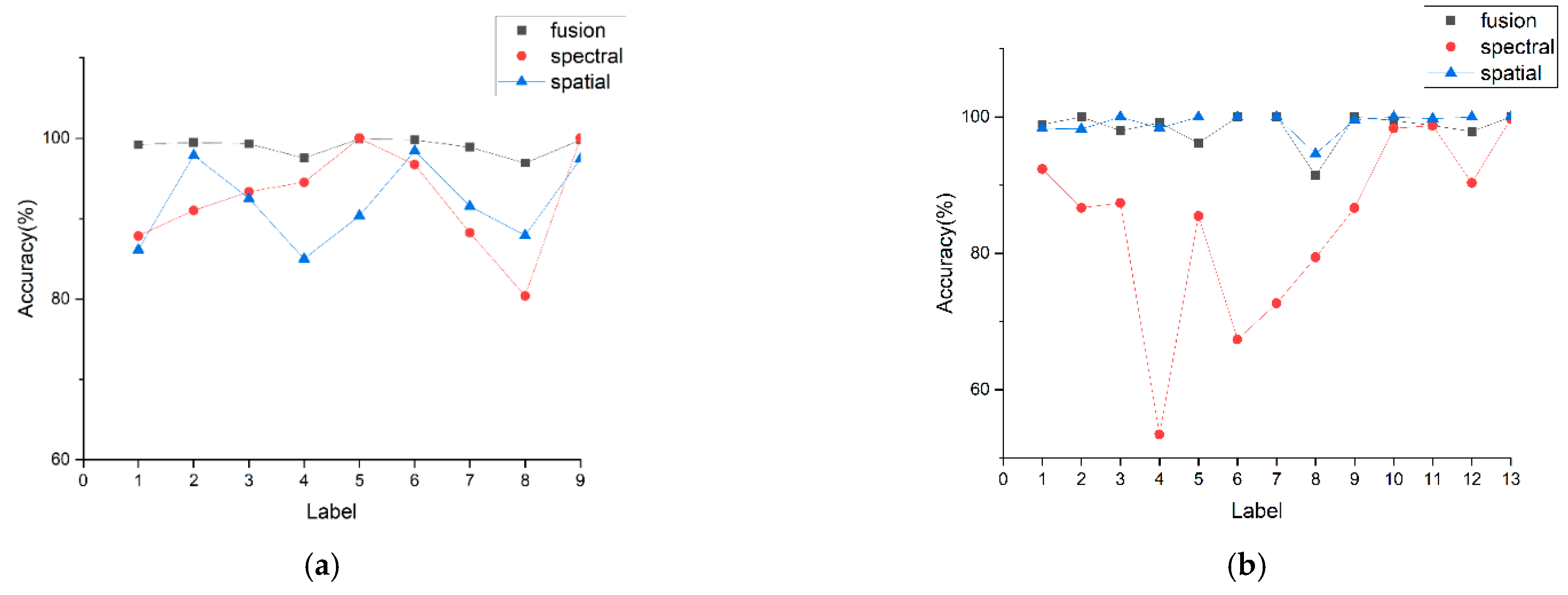
One of the important reasons why the framework can achieve high classification accuracy is the idea of feature fusion. To verify the impact of different features on hyperspectral imagery classification, we use spectral features, spatial features, and fusion features as feature vectors, respectively, to train the SVM classifier and check the differences in classification accuracy. Figure 4 shows the classification results obtained by different feature types for the Pavia University datasets and Kennedy Space Center dataset. When the fusion feature is used as a feature vector, the best classification effect can be achieved. However, when there are only spectral features or spatial features, the classification accuracy decreases to varying degrees. Generally, it is reasonable to believe that when the feature information of a certain category is more fully mined, the resulting higher-dimensional feature vector has a more positive impact on the classification and therefore improves the classification accuracy. For different types of label, the classification accuracy of fusion feature has less fluctuation, which enhances the robustness of the framework.

The spatial features extracted by the DeepLab v3+ network have a positive impact on subsequent classification. The classification framework based on DeepLab v3+ surpassed CNN, ELM, and other algorithms in this experiment. It extracted the explicit or implicit relationship in space between each category of pixels and other pixels. The spatial features obtained satisfy the requirements of classification tasks, which also indirectly reflects the powerful spatial feature extraction capabilities of DeepLab v3+ and its wide applicability.

3.3. Generalization Verification

In an ideal situation, the image after the principal component extraction would be fed to the DeepLab v3+ neural network, and the spatial feature information would be obtained after training. However, in real scenes, many data to be classified are unlabeled, which requires that the trained neural network can also extract spatial feature from unseen images. Therefore, two labeled pictures in the HyRANK dataset are used to verify the generalization of the feature extraction network. Among them, the picture Loukia is used as a known dataset, and the picture Dioni is used as an unknown dataset. After feature extraction and fusion, the classification results are obtained.

Table 6. Classification accuracy (%) for Loukia and Dioni.

	Loukia					Dioni
Class	KNN	Logistic Regression	Decision Tree	Naive Bayesian Model	SVM	KNN	Logistic Regression	Decision Tree	Naive Bayesian Model	SVM
1	68.06	40.15	18.88	18.03	67.82	85.66	79.19	49.04	40.40	92.81
2	100	100	50	100	100	93.89	94.89	31.33	100	100
3	83.81	73.03	51.45	40.94	90.4	98.55	74.14	49.58	54.10	95.73
4	59.32	72.73	10.87	100	100	81.44	88.89	19.37	78.26	100
5	81.49	66.11	45.29	35.73	82.87	94.63	78.60	61.87	62.60	94.57
6	81.48	46.07	32.02	15.47	100	\	\	\	\	\
7	77.33	66.67	39.32	40.34	94.08	97.43	92.14	81.95	63.89	100
8	72.98	67.16	50.46	53.84	82.19	\	\	\	\	\
9	74.22	71.08	62.85	80.10	78.02	97.26	90.82	87.79	88.45	95.34
10	83.06	69.7	63.53	73.31	73.2	96.78	87.90	83.64	87.34	93.84
11	89.66	76.69	49.78	49.40	96.25	95.42	84.01	60.58	72.53	90.79
12	97.31	84.54	69.60	57.93	95.51	99.55	96.84	82.33	88.99	100
13	100	99.60	95.91	100	100	98.51	99.66	97.89	99.04	100
14	100	99.01	79.33	91.82	100	99.70	96.82	91.74	59.77	100
OA	81.45	73.92	60.70	52.76	82.39	96.06	88.00	77.26	76.90	94.92
AA	83.48	73.75	51.38	61.21	90.03	94.90	88.66	66.43	74.61	96.92
Kappa	77.80	68.72	53.43	47.66	78.69	95.10	85.06	71.92	71.80	93.66

represents the classification result of the known dataset Loukia and the unknown dataset Dioni using different classifiers.

The results show that the classification accuracy of Loukia is relatively mediocre. The reason is that the same feature category is scattered and each area is small. Different types of feature categories are mixed together, which brings great difficulty to the classification. Apart from this, the difference in spectral characteristics between different types of ground features is not obvious enough, which is also a reason for the poor classification.

However, although Dioni is a new dataset for the feature extraction network, the framework can still perform the classification task excellently. Facing the same environmental conditions, the framework has a strong classification ability for hyperspectral data collected by the same sensor. Therefore, the framework has strong generalization ability and application prospects.

3.4. Visualization

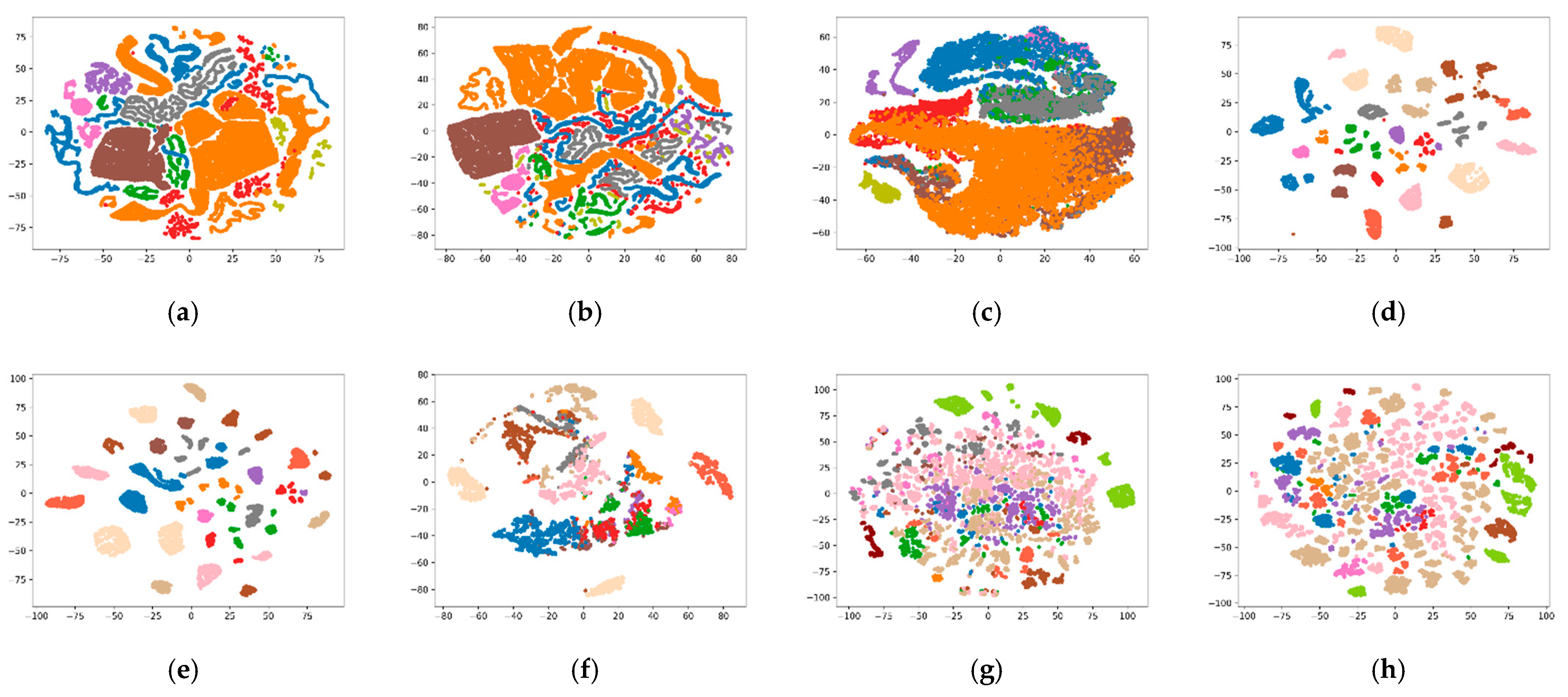
To intuitively understand the impact of different factors on the classification, we also have done a series of data visualization. First, we use the visualization tool TSNE to reduce the dimensionality of the feature vector of each pixel to two dimensions, and project it to a 2-D coordinate system. By observing the degree of dispersion in each category, we can judge the difficulty of classification.

Figure 5 represents the distribution effects of pixels with spectral, spatial, and fusion features for the Pavia University dataset, Kennedy Space Center dataset, and HyRANK dataset. As we can see from the figure, the pixels with fusion features have the best degree of aggregation in each category, and the overlapping area between different categories is the least, making it is easy to be classified. This shows the importance and efficiency of the feature fusion method in hyperspectral imagery classification. Similarly, the degree of aggregation of Dioni’s pixel distribution is better than that of Loukia.

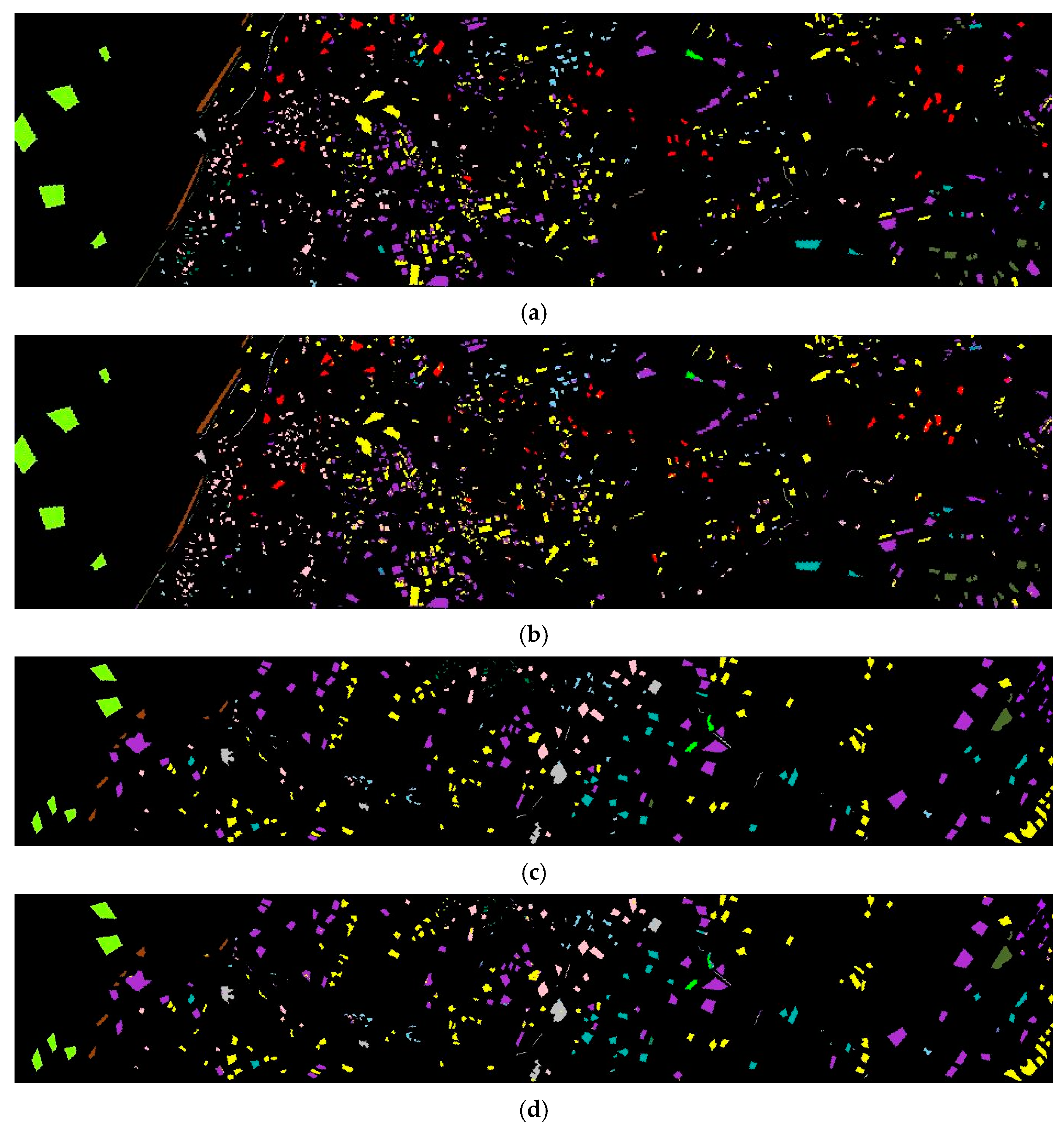
Figure 6 and Figure 7, respectively, represent the prediction classification maps for the Pavia University dataset and Kennedy Space Center dataset with different factors. After the spatial feature extraction of the DeepLab v3+ network, the feature fusion of spatial and spectral features, and the use of SVM classifiers for fitting and prediction produce the best classification map. Figure 8 represents the prediction classification maps for Loukia and Dioni. Compared to Dioni, the distribution of categories in Loukia is more scattered and complex; therefore, it is more difficult to be classifier.

4. Conclusions

In this paper, a hyperspectral imagery classification framework based on DeepLab v3+ is proposed. In the framework, DeepLab v3+ neural network is used as the spatial feature extraction method, and the spatial and spectral features are used for feature fusion. Finally, the SVM classifier is selected as the classification method among several classifiers. Compared with traditional machine learning algorithms and convolutional neural network algorithms in the same kind of dataset, our proposed framework not only significantly improves the classification accuracy but also improves the classification efficiency. Experimental results show that DeepLab v3+ has excellent spatial feature extraction capabilities and applicability in hyperspectral imagery classification, and the feature fusion method can effectively improve the classification accuracy of hyperspectral imagery. Experiments have shown that the framework proposed in this paper has good generalization, and the classification accuracy is better than other traditional machine-learning algorithms and deep-learning algorithms.

References

1. Harsanyi, J.C.; Chang, C.I. Hyperspectral image classification and dimensionality reduction: An orthogonal subspace projection approach. IEEE Trans. Geosci. Remote Sens. 1994, 32, 779–785. [Google Scholar] [CrossRef] [Green Version]
2. Licciardi, G.; Marpu, P.R.; Chanussot, J.; Benediktsson, J.A. Linear versus nonlinear PCA for the classification of hyperspectral data based on the extended morphological profiles. IEEE Geosci. Remote Sens. Lett. 2011, 9, 447–451. [Google Scholar] [CrossRef] [Green Version]
3. Green, A.A.; Craig, M.D.; Shi, C. The application of the minimum noise fraction transform to the compression and cleaning of hyper-spectral remote sensing data. Int. Geosci. Remote Sens. Symp. IEEE 1988, 3, 1807. [Google Scholar]
4. Balasubramanian, M.; Schwartz, E.L.; Tenenbaum, J.B.; de Silva, V.; Langford, J.C. The lsomap algorithm and topological stability. Science 2002, 295, 7. [Google Scholar] [CrossRef] [PubMed] [Green Version]
5. Belkin, M.; Niyogi, P. Laplacian eigenmaps and spectral techniques for embedding and clustering. Adv. Neural Inf. Process. Syst. 2001, 14, 585–591. [Google Scholar]
6. Chen, Y.; Jiang, H.; Li, C.; Jia, X.; Ghamisi, P. Deep feature extraction and classification of hyperspectral images based on convolutional neural networks. IEEE Trans. Geosci. Remote Sens. 2016, 54, 6232–6251. [Google Scholar] [CrossRef] [Green Version]
7. Ying, L.; Haokui, Z.; Qiang, S. Spectral–spatial classification of hyperspectral imagery with 3D convolutional neural network. Remote Sens. 2017, 9, 67. [Google Scholar]
8. Samaniego, L.; Bárdossy, A.; Schulz, K. Supervised classification of remotely sensed imagery using a modified k-NN technique. IEEE Trans. Geosci. Remote Sens. 2008, 46, 2112–2125. [Google Scholar] [CrossRef]
9. Hasanlou, M.; Samadzadegan, F.; Homayouni, S. SVM-based hyperspectral image classification using intrinsic dimension. Arab. J. Geosci. 2015, 8, 477–487. [Google Scholar] [CrossRef]
10. Kang, X.; Li, S.; Benediktsson, J.A. Spectral-spatial hyperspectral image classification with Edge-Preserving Filtering. IEEE Trans. Geosci. Remote Sens. 2014, 52, 2666–2677. [Google Scholar] [CrossRef]
11. Chen, X.; Wei, Z.; Li, M.; Rocca, P. A review of deep learning approaches for inverse scattering problems (Invited Review). Prog. Electromagn. Res. 2020, 167, 67–81. [Google Scholar] [CrossRef]
12. Ma, T.; Lyu, H.; Liu, J.; Xia, Y.; Qian, C.; Evans, J.; Xu, W.; Hu, J.; Hu, S.; He, S. Distinguishing bipolar depression from major depressive disorder using fNIRS and deep neural network. Prog. Electromagn. Res. 2020, 169, 73–86. [Google Scholar] [CrossRef]
13. Fajardo, J.E.; Galván, J.; Vericat, F.; Carlevaro, C.M.; Irastorza, R.M. Phaseless microwave imaging of dielectric cylinders: An artificial neural networks-based approach. Prog. Electromagn. Res. 2019, 166, 95–105. [Google Scholar] [CrossRef] [Green Version]
14. Chen, Y.; Lin, Z.; Zhao, X.; Wang, G.; Gu, Y. Deep learning-based classification of hyperspectral data. IEEE J. Sel. Top. Appl. Earth Obs. Remote Sens. 2017, 7, 2094–2107. [Google Scholar] [CrossRef]
15. Jonathan, L.; Shelhamer, E.; Darrell, T. Fully convolutional networks for semantic segmentation. IEEE Trans. Pattern Anal. Mach. Intell. 2015, 39, 640–651. [Google Scholar]
16. Li, J.; Zhao, X.; Li, Y.; Du, Q.; Xi, B.; Hu, J. Classification of hyperspectral imagery using a new fully convolutional neural network. IEEE Geosci. Remote Sens. Lett. 2018, 15, 292–296. [Google Scholar] [CrossRef]
17. Chen, L.; Zhu, Y.; Papandreou, G.; Schroff, F.; Adam, H. Encoder-decoder with atrous separable convolution for semantic image segmentation. ECCV 2018, 2018, 801–818. [Google Scholar]
18. Yu, F.; Koltun, V. Multi-scale context aggregation by dilated convolutions. In Proceedings of the International Conference on Learning Representations 2016, San Juan​, Puerto Rico, 2–4 May 2016; pp. 397–410. [Google Scholar]
19. He, K.; Zhang, X.; Ren, S.; Sun, J. Spatial pyramid pooling in deep convolutional networks for visual recognition. IEEE Trans. Pattern Anal. Mach. Intell. 2014, 37, 1904–1916. [Google Scholar] [CrossRef] [PubMed] [Green Version]
20. Niu, Z.; Liu, W.; Zhao, J.; Jiang, G. DeepLab-based spatial feature extraction for hyperspectral image classification. IEEE Geosci. Remote Sens. Lett. 2019, 16, 251–255. [Google Scholar] [CrossRef]
21. Pavia University Hyperspectral Satellite Dataset from the Telecommunications and Remote Sensing Laboratory, Ipavia University (Italy). Available online: https://www.kaggle.com/abhijeetgo/paviauniversity (accessed on 21 June 2018).
22. Kennedy Space Center Hyperspectral Satellite Dataset from the NASA AVIRIS (Airborne Visible/Infrared Imaging Spectrometer) Instrument. Available online: http://www.ehu.eus/ccwintco/index.php/Hyperspectral_Remote_Sensing_Scenes (accessed on 23 March 1996).
23. HyRANK Hyperspectral Satellite Dataset I (Version v001) [Data Set]. Available online: http://doi.org/10.5281/zenodo.1222202 (accessed on 20 April 2008).
Figure 1. Illustrations of (a) convolution and (b) atrous convolution.
Applsci 11 05703 g001
Figure 2. Illustration of (a) spatial pyramid pooling (SPP) structure and (b) atrous spatial pyramid pooling (ASPP) structure in DeepLab v3+.
Applsci 11 05703 g002
Figure 3. Schematic depictions of the architecture of (a) DeepLab v3+ and overall architecture of the (b) proposed framework.
Applsci 11 05703 g003aApplsci 11 05703 g003b
Figure 4. Classification accuracy versus label with fusion feature, spectral feature, and spatial feature for the (a) Pavia University dataset and (b) Kennedy Space Center dataset.
Applsci 11 05703 g004
Figure 5. Feature distribution of pixels with fusion feature, spectral feature and spatial feature for the Pavia University dataset and Kennedy Space Center, and fusion feature for HyRANK dataset. (a) Fusion feature-PaviaU; (b) spatial feature-PaviaU; (c) spectral feature-PaviaU; (d) fusion feature-KSC; (e) spatial feature-KSC; (f) spectral feature-KSC; (g) fusion feature-Loukia; and (h) fusion feature-Dioni.
Applsci 11 05703 g005
Figure 6. Feature maps achieved by using different classifiers and features for the Pavia University dataset. (a) DT—fusion feature; (b) KNN—fusion feature; (c) LR—fusion feature; (d) NBM—fusion feature; (e) SVM—fusion feature; (f) SVM—spatial feature; and (g) SVM—spectral feature.
Applsci 11 05703 g006
Figure 7. Feature maps achieved by using different classifiers and features for the Kennedy Space Center dataset. (a) DT—fusion feature, (b) KNN—fusion feature, (c) LR—fusion feature, (d) NBM—fusion feature; (e) SVM—fusion feature; (f) SVM—spatial feature; and (g) SVM—spectral feature.
Applsci 11 05703 g007
Figure 8. Feature maps produced using SVM classifiers and fusion features for the HyRANK dataset. (a) The ground truth of Loukia. (b) The predicted feature map for Loukia. (c) The ground truth of Dioni. (d) The predicted feature map for Dioni.
Applsci 11 05703 g008