Deeply-Supervised 3D Convolutional Neural Networks for Automated Ovary and Follicle Detection from Ultrasound Volumes

Abstract

Automated detection of ovarian follicles in ultrasound images is much appreciated when its effectiveness is comparable with the experts’ annotations. Today’s best methods estimate follicles notably worse than the experts. This paper describes the development of two-stage deeply-supervised 3D Convolutional Neural Networks (CNN) based on the established U-Net. Either the entire U-Net or specific parts of the U-Net decoder were replicated in order to integrate the prior knowledge into the detection. Methods were trained end-to-end by follicle detection, while transfer learning was employed for ovary detection. The USOVA3D database of annotated ultrasound volumes, with its verification protocol, was used to verify the effectiveness. In follicle detection, the proposed methods estimate follicles up to 2.9% more accurately than the compared methods. With our two-stage CNNs trained by transfer learning, the effectiveness of ovary detection surpasses the up-to-date automated detection methods by about 7.6%. The obtained results demonstrated that our methods estimate follicles only slightly worse than the experts, while the ovaries are detected almost as accurately as by the experts. Statistical analysis of 50 repetitions of CNN model training proved that the training is stable, and that the effectiveness improvements are not only due to random initialisation. Our deeply-supervised 3D CNNs can be adapted easily to other problem domains.

1. Introduction

A sexually mature female has two almond-shaped ovaries about the size of a large grape, one on each side of the uterus. The human ovary consists of a surface, an inner medulla and outer cortex, with indistinct boundaries between the latter two. The medulla contains the blood vessels, lymphatic vessels and nerves, while the cortex embraces the developing follicles [1]. The follicle is certainly a very important part of the ovary. It is similar to a small sac filled with liquid, holding one immature egg (ovum). The ovary contains thousands of follicles. A few selected follicles begin to develop (grow) during each woman’s menstrual cycle. At the end of the menstrual cycle, typically, only one of these follicles reaches maturity and the rest deteriorate. This mature, so-called dominant, follicle breaks open and releases the egg from the ovary for possible fertilisation [1,2].

Monitoring changes in the ovary, especially follicle growth dynamics during the menstrual cycle, is crucial for the fields of Obstetrics and Gynaecology (e.g., for In-Vitro Fertilisation). On the other hand, the measurement of ovarian volume has been shown to be a useful indirect indicator of the ovarian reserve in women of reproductive age, in the diagnosis and management of a number of disorders of puberty and adult reproductive function, and is under investigation as a screening tool for ovarian cancer [3]. Clinicians today use non-invasive ultrasound devices regularly for these purposes, with which they conduct frequent examinations of patients. Modern ultrasound devices support 3D recording, and contain computer algorithms that help Sonographers recognise the observed 3D structures. The use of 3D ultrasound devices allows us to capture the entire ovary and follicles in a single sweep, which may take seconds to complete, unlike 2D ultrasound devices, where much more time is needed to capture the imaging material. Besides, the 3D recording enables a more detailed survey of the ovary and follicles compared to 2D ultrasound. Several display modes and standardised examinations permit the observation of ovary and follicles in controlled planes and rendered images from different (optimal) angles. In this way, we can notice the peculiarities of the ovary and follicles faster and more accurately [4].

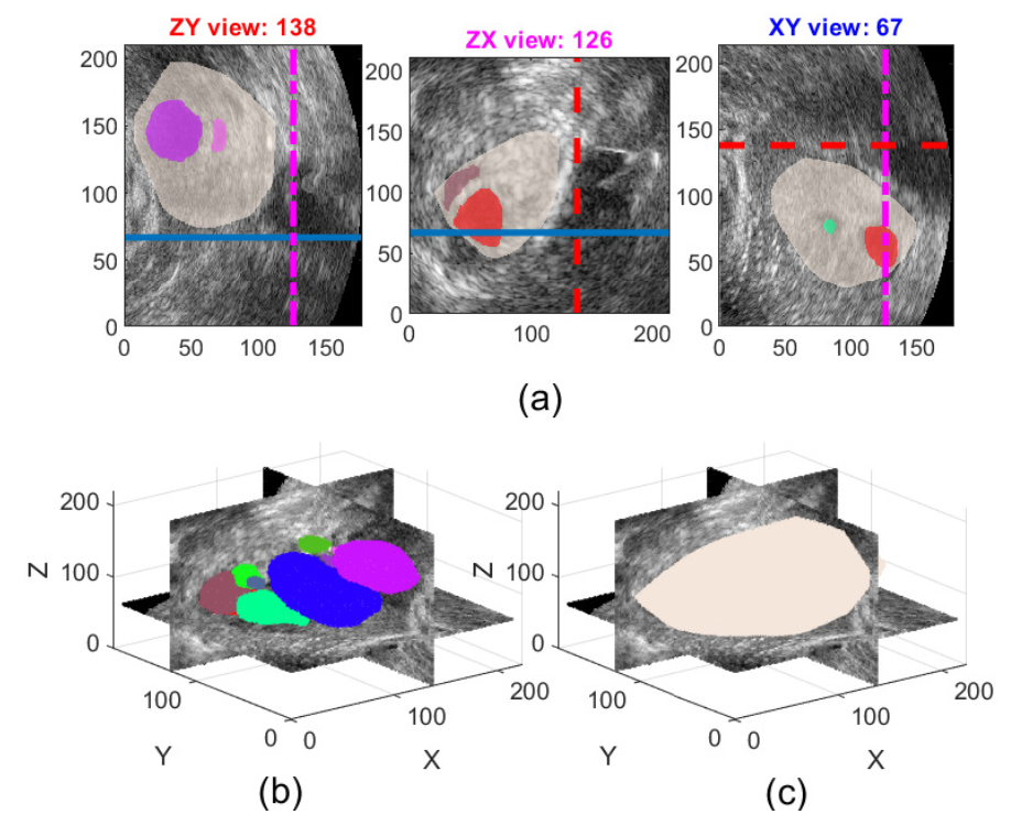
The ovarian follicles manifest on ultrasound images (volumes) as darker regions (volumes) on a brighter background. Figure 1 depicts a sample 3D ovarian ultrasound image with follicles (coloured) inside an ovary (ochre) annotated by an expert in 2D views of selected cross-sections through the volume (top row) and in a 3D view (bottom row).

Manual, or non-automated follicle observing in a day-to-day manner is very laborious and time-consuming, and due to the routine nature of the work it can also lead to inaccuracies. Already in the 90s of the last century, computer procedures for follicle detection and recognition began to appear, initially for the 2D ultrasound images [5]. This research and application field has been evolving constantly with the introduction of increasingly efficient and accurate automated or semi-automated detection algorithms, respectively. Thus, we have witnessed a development from simple 2D detection methods in the 1990s, such as solutions based on heuristic graph searching, optimal thresholding, cellular automata and 2D region growing, all the way to sophisticated approaches at the beginning of the 21st century, such as are knowledge-based methods, methods based on cellular neural networks and the Kalman filter [5,6]. The efficiency (usually sensitivity and precision were used as the metrics) and accuracy (metrics mean absolute distance between the detected and annotated follicle) of detection approaches have increased with this development. 3D ultrasound devices began to appear massively around 2000, and in a few years became the de facto Standard in the field of Obstetrics and Gynaecology. Simultaneously, the development of follicle detection approaches has shifted from methods designed to process 2D cross-sections through the ovary to true 3D detection methods that process 3D ovarian ultrasound volumes as a whole. Among them we find successful methods based either on continuous wavelets, levels sets, or on trained probabilistic frameworks of ovary and follicle models [5,7]. The proprietary semi-automated detection algorithm SonoAVC [8], incorporated in the General Electric ultrasound devices designed for automated volume calculation, should also be pointed out. The 3D follicle detection method based on the Directional 3D Wavelet Transform (3D DWT) [9], developed by our research group, has proven to be also very efficient and accurate.

Recently, Deep Learning based approaches have been proposed for follicle and ovary detection. The CR-Unet network [10] upgraded a 2D U-Net architecture by spatial Recurrent Neural Network (RNN) modules. These RNN modules were used to learn large scale spatial features in the segmentation model. The model was trained to detect ovaries and follicles simultaneously as a three class segmentation problem. This model was, indeed, trained on 2D ultrasound slices, but can also be applied in a slice-by-slice manner to 3D volumes. The S-Net network [11] also utilised the 2D U-Net, with the difference that several slices of a 3D volume were processed at once. Such processing enabled the extraction of additional 3D information, and, thus, reduced discontinuities in the 3D segments. S-Net treated ovary and follicle detection as two binary segmentation problems. It used a special composite Binary Cross Entropy loss function that gave an additional penalty to follicle detections outside the ovary. Both mentioned Deep Neural Networks were trained and evaluated on proprietary databases, which makes direct comparisons with these results difficult. However, the methods in [10,11] were compared directly, demonstrating S-Net [11] to be superior.

After a brief review, we concluded that this research field is a mature, but still active field, as the development of improved computer follicle detection approaches still challenges many researchers [5,9,10,11,12].

Already in our review article [5] we identified the problem of unbiased comparison of follicle detection algorithms. In order to validate the solutions, different research groups, namely, use all sorts of metrics, evaluated on their own image datasets, in which the follicles (ovaries) are annotated manually by experts according to their own protocol. Such indefiniteness limits the objective comparison of different follicle-detection approaches. In our previous work [7], we therefore published the USOVA3D public database of annotated 3D ultrasound images of ovaries, which was supplemented with a precisely specified verification protocol for unbiased assessment of general detection algorithms. Additionally, two baseline algorithms were introduced for follicle and ovary detection. The first algorithm, 3D DWT, uses heuristic features and a classical approach to designing algorithms. In fact, it is a small upgrade of our most efficient follicle detection method to date [9]. The second baseline algorithm, 2D UNET, demonstrates modern algorithm designing based on Deep Learning, the Convolutional Neural Networks (CNN) theory, and established 2D U-Net architecture. Both algorithms were evaluated on the USOVA3D testing set, and the baseline results (i.e., scores) were established for the follicle and ovary detection efficiency [7]. We also confirmed by thorough analysis that the USOVA3D database can be a reliable source for developing new detection methods.

We deal with the development of effective learning-based object detection approaches in 3D medical imaging data using 3D Convolutional Neural Networks in this research. Although 2D CNN-based detection methods that process volumes in a slice-by-slice manner and then combine partial results into a whole, generally tend to be superior in respect of the ‘true’ 3D CNN-based detection methods that process volumes as a whole [13] (the reasons are often the need for an extremely large number of training samples and the huge computational complexity of 3D CNNs), the opposite will be demonstrated in this work. On the case of follicle and ovary detection in ovarian ultrasound volumes, we will confirm experimentally that it is possible to develop sophisticated 3D CNN-based methods that surpass 2D CNN-based methods and 3D methods based on ‘hand-crafted’ features. The development and verification of 3D detection procedures will be conducted by using the USOVA3D public database, which is basically a relatively small database. 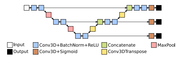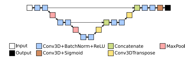It is usually the lack of data that is the main reason for the lower efficiency of 3D CNN-based detection methods [13]. However, it will be proven in this research that we can develop an effective 3D detection method through appropriately supervised learning, despite the relatively small training set. This paper thus introduces advanced solutions based on three-dimensional CNNs for the follicle and ovary detection in ovarian ultrasound volumes. 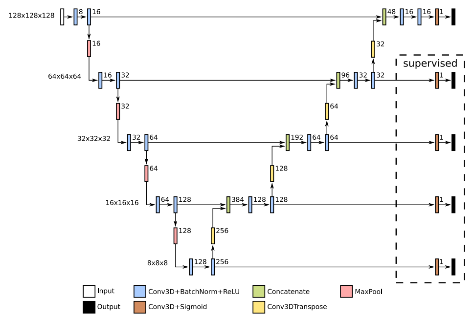Our solutions are based on the established U-Net architecture [14,15]. We have developed advanced methods for 3D object detection in volumes by using the Deep Supervision technique [16], and by replication of either the entire U-Net architecture or certain parts of the U-Net decoder. The proposed approaches were designed primarily for 3D follicle and ovary detection in ultrasound volumes. The effectiveness of the proposed methods was verified by using the USOVA3D database.

The contribution of this research work is summarised in:

• The development of sophisticated two-stage CNN-based algorithms for 3D object detection, whereat the algorithms are built on the U-Net architecture and Deep Supervision;
• Introduction of the most effective 3D algorithms for follicle and ovary detection, obtained by appropriately controlled training;
• Effectiveness assessment of CNN-based object detection approaches by statistical evaluation of multiple model training repetitions.

This article is structured as follows. A short overview of the USOVA3D public database and employed evaluation protocol is given in Section 2. Novel 3D object detection algorithms based on the U-Net architecture are described in detail in Section 3. In addition, guidelines are provided on how to adapt these methods to detect follicles and ovaries. Section 4 presents some of the results obtained on the USOVA3D database, followed by Section 5, which emphasises certain aspects of our detection methods. Section 6 concludes this paper briefly with some hints about future work.

2. Review of the USOVA3D Public Database and the Evaluation Protocol

The USOVA3D public database of annotated 3D ultrasound images of ovaries is summarised briefly in this sequel, while details can be found in our previous work [7]. The database consists of 35 entries, which are predivided into training (16 entries) and a testing (19 entries) sets. Each entry contains 5 volumes (3D images), namely, the original ovarian ultrasound volume, two times manually annotated ovary and two times manually annotated follicles. Manual annotations (segmentations) were provided independently by two experienced medical experts (i.e., by rater 1 and rater 2). Its volume size is between $[101\dots 229]\times [89\dots 193]\times [115\dots 247]$ voxels, with the voxel dimensions 0.2 mm × 0.2 mm × 0.2 mm. The raters’ manual annotations are considered as ‘ground truth’. The USOVA3D database is accessible at the web address: https://usova3d.um.si (accessed on 1 January 2022).

As is widely accepted, the use of training data is foreseen for the development of detection algorithms, and a testing set is intended for an efficiency evaluation. The USOVA3D database introduces a small change in respect of this established concept. Only the original ovarian ultrasound volumes are available to researchers in the testing set, but not the manual annotations of the ovaries and follicles. Validation of the new detection method is, therefore, performed exclusively using the USOVA3D services on the USOVA3D portal, as the ‘ground truth’ for the testing set is stored on the USOVA3D portal only, and is not part of the publicly accessible USOVA3D database. Such design of the USOVA3D database leads to a more fair validation and comparison of algorithms.

2.1. Evaluation Protocol

A general evaluation protocol for the unbiased assessment of detection algorithms was also developed in [7] as a supplement to the USOVA3D database. This evaluation returns an overall score of the detection algorithm, ${\xi }_{alg}$, which takes into account several aspects of detection performance and accuracy (5 metrics) on all testing data. At the same time, a detection that deviates more strongly from the average detection performance on the testing set is considered in the overall score with a smaller weight. The advantage of our protocol is that we obtain a single effectiveness estimate for each method over all metrics, all raters, and all testing data, and, therefore, the methods do not need to be re-ranked according to each of the individual metrics.

The overall algorithm score is determined as described in this sequel. An individual detection algorithm is validated on the USOVA3D testing set in our research. Detection effectiveness and accuracy are first evaluated using 5 metrics separately for each of the 19 entries in the testing set. The following metrics are calculated: (i) Product of sensitivity and precision ((1) in [7]), (ii) Product ${\rho }_1{\rho }_2$, (iii) The ratio of the total volume of correctly detected objects (follicles or ovary) and the total volume of all the referential objects ((2) in [7]), (iv) The mean Euclidean distance (in voxels) between the surfaces of correctly detected and referential objects ((3) in [7]), and (v) The mean absolute difference (in voxels) between the diameters of equivalent spheres that have the same volumes as the detected and referential objects ((4) in [7]). The first three metrics have values between 0 and 1, while the last two metrics are normalised to the interval $[0,1]$. All five metrics are then summed and multiplied by 20 to give the so-called combined score, i.e., a value between 0 and 100 for each entry (volume) in the testing set.

The USOVA3D database was annotated manually by 2 raters. The segmentation result for each entry in the testing set is, therefore, compared to the annotations of both raters. The metrics for those objects in the volume where the raters agreed in the annotations are considered with greater weight than for objects where there was disagreement between both the raters. The final score, ${\xi }_{vol}$, for an individual entry (volume) in the testing set is calculated from the combined scores in this way. There are currently 19 entries in the USOVA3D testing set, which means we get 19 final scores ${\xi }_{vol}$. Finally, the overall algorithm score, ${\xi }_{alg}$, is determined by statistical analysis of the 19 final scores ${\xi }_{vol}$, calculated for all volumes in the USOVA3D testing set.

An overall algorithm score was introduced primarily for ranking the detection algorithms in respect of their performance. The overall score ${\xi }_{alg}$ equal to 100 would have a perfect detection algorithm, while ${\xi }_{alg}=0$ would be assigned to the worst detection algorithm possible. The evaluation protocol summarised here is explained in detail in [7]. Auxiliary routines that implement this evaluation protocol are available on the USOVA3D portal.

This evaluation protocol can also be used with a small extension to assess inter-rater variability. In the case of the USOVA3D database, at first we take the annotations of the first rater as ‘ground truth’ and the annotations of the second rater as the detection algorithm results, and then calculate the overall score (${\xi }_{rater2}$ score, that measures the variability of rater 2’s annotations with respect to rater 1). Afterwards we reverse the raters’ roles and repeat the calculation (${\xi }_{rater1}$ score). The inter-rater variability and reliability of the USOVA3D database has been analysed carefully in [7].

3. Computational Methods

3.1. U-Net Architecture

Our proposed solutions are based on the U-Net architecture [14,15], modified for 3D volumetric data [17]. We chose U-Net as it has been proven as a baseline for the USOVA3D database for ovary detection [7]. It is also a popular architecture for the problem of follicle and ovary detection in ovarian ultrasound data [10,11].

The U-Net architecture in 3D space is identical to that in 2D, utilising 3D layers and/or 3D building blocks instead of their 2D counterparts. The basic U-Net architecture is constructed from a series of down-sampling encoders, followed by up sampling decoders organised in layers representing the scale of the feature map. An example is shown in Figure 2.

Each encoder contains a series of two convolution blocks and a max pooling layer. Each convolution block consists of a convolution, batch normalisation and ReLU activation. The output of the max pooling is used as the input of the next encoder, while the output of the second convolution block is passed to the decoder. As the size of the feature map decreases with pooling, the number of channels is doubled in the second convolution block. There is the encoder with only two convolution blocks and no pooling at the lowest level in Figure 2.

The output is then passed to the first decoder’s transposed convolution layer. Each decoder consists of a transposed convolution, concatenation and two convolution blocks. The transposed convolution up-samples the output of the previous decoder, while the concatenation combines this with the output of the second convolution block of the encoder on the same scale level. Lastly, the output of the final decoder’s convolution block is processed by a classification block constructed of a convolution layer and sigmoid activation.

The outputs of the last encoder and each decoder are feature maps optimised for the targeted segmentation task. Feature maps from the final decoder are then passed through a classification layer, a convolution with a sigmoid transfer function, to produce the targeted segmentation map.

3.2. Deep Supervision

Adding and optimising intermediate outputs at multiple levels of a neural network has been shown to improve training stability and performance. The Deep Supervision introduced in [16] is an example of such successful approach.

Deep Supervision is often used in U-Net [10,11,18,19]. Figure 3 depicts an example of the U-Net architecture using Deep Supervision. Additional classification layers are added to the feature maps at each scale. Usually, these outputs are resampled to match the sampling at the original input size, a loss is computed for each of them, and a final combined loss over all layers is produced using a weighted sum. The weights are adjusted commonly for each layer.

The predicted outputs on each level remain as they are in our implementation of Deep Supervision, while the ground truth labels are subsampled to match the outputs’ sizes. This reduces the memory requirements during training. No additional weighting scheme is used to balance the loss of different outputs. The losses are summed up simply.

3.3. U-Net Extensions

Quite a few studies have substantiated that detecting ovaries is a much more difficult problem than detecting follicles in ultrasound images/volumes [5]. This is reflected in the much greater inter-rater variability of ovary annotations in respect to the variability of follicle annotations in the USOVA3D database [7]. Through experimentation, we found that training an independent U-Net network either to predict solely ovaries, or jointly, to predict ovaries and follicles, resulted in poorly detected ovaries and in a lower precision metric if follicles were detected as well. On the other hand, training the U-Net for follicle detection only improved results (i.e., recognition rate and accuracy).

It is known from the anatomy that the follicles are always located inside the ovary. In this work, we aim to exploit this relationship and the follicle segmentation results to improve the ovary segmentation. We developed a two-stage architecture for follicle and ovary detection. Follicles are detected in the first stage, and the prior knowledge of the ovary-follicles relationship is utilised in the second stage. The idea is similar to the 3D DWT baseline function [7], except that this baseline function did not perform well when detecting ovaries.

We have implemented two different extensions of the U-Net architecture to exploit the ovary-follicles relationship. Both CNNs consist of one base U-Net network trained to detect follicles. The extension is then applied to this network to predict ovary segments.

The first extension, EXT 1, shown in Figure 4, brings in a full additional U-Net network. The implementation is trivial and straightforward. An output of the first network, i.e., a segmentation map for follicles, is concatenated with the input volume and passed to the second U-Net network. By providing the segmentation maps of follicles we submit seeding information about potential ovary location to the second network. Such information focuses the second U-Net on the important parts of the input volume.

The second extension, EXT 2, not only utilises the segmentation of follicles, but also exploits the extracted features used to predict such segmentation. The EXT 2 extension is depicted in Figure 5. The predictive features at each level of the base U-Net are passed to the same level of the second network aimed for detecting the ovaries. These features have already gone through the encoders of the base U-Net. However, these features have been optimised for the follicle detection. In order to adapt them for ovary detection, we introduced additional convolution blocks at the lowest layer, and additional decoders on the higher levels of the second CNN.

Additional outputs are added to both extensions, as shown in grey in Figure 4 and Figure 5 when training with Deep Supervision.

3.4. Network Parameters

The multi-scale U-Net architecture is parametrised by a scale, convolution kernel size, and a number of channels in the first convolution block. In our experiments, we used a scale equal to 5, kernels of 3 × 3 × 3 for all convolution and transposed convolution layers, and 8 channels for the initial convolution block. Every second convolution block in the encoder doubles the number of channels. The network architecture is detailed in Figure 6. When using Deep Supervision additional outputs were added, specified at the right of the Figure.

Our first proposed U-Net extension, EXT 1, concatenates the output of the basic U-Net with the input volume, thus creating a 2-channel input. Such conglomerate is then passed to the U-Net, as specified in Figure 6. The second proposed U-Net extension, EXT 2, introduces additional decoders to the network. These are identical to the decoders in the original U-Net. The extension layers are specified in Figure 7, and are connected to the original U-Net layers (see also Figure 6). If Deep Supervision is employed, then additional outputs must be introduced to the CNNs. These additional outputs are specified at the right of Figure 6 and Figure 7.

3.5. Follicle and Ovary Detection

All CNNs described in this article can be adapted easily to detect follicles and ovaries. First, inputs (i.e., ovarian ultrasound volumes) and expected outputs (i.e., ground truth for follicles and ovaries) need to be prepared properly, followed by appropriate Neural Network training. In the case of the USOVA3D database data are already prepared, and it is just a matter of implementation details of how the data are fed into the CNN. In this sequel, we will provide some guidance on how to train the presented CNNs to be more focused and controlled. Special emphasis will be placed on ovary detection by using the U-Net extensions.

3.5.1. Transfer Learning

The proposed extended U-Nets can be trained definitively end-to-end to predict both ovary and follicles. However, such simultaneous training for both types of objects can have a negative impact on the ultimate detection effectiveness. We are dealing in both stages with the optimisation, and therefore there may be a trade-off between the successfulness of follicle and ovary detection. To avoid this problem, we trained the first stage or follicle detection independently of the second stage. Afterwards, the weights of the trained CNN from the first stage were frozen (i.e., the network was not trained, just weights were loaded) and the weights for the second stage network were only trained/adapted. As already mentioned, the second stage of the extended U-Net is aimed to detect ovaries.

The described approach is similar to the popular Transfer Learning techniques [20,21], where weights of particular layers of a trained network on one problem are reused in the similar network designed for a different application problem.

3.5.2. Loss Function

The proposed CNNs were trained by using the same loss function as defined in [7]. The loss function was left unchanged intentionally, as we wanted to demonstrate that all the improvements were solely due to the CNN architecture modifications and supervised training. Our final loss function L is, therefore, a combination of the binary cross-entropy loss ($L_{Ent}$), the loss based on the Dice Similarity Coefficient ($L_{DSC}$) and the loss based on ${\rho }_1{\rho }_2$ product ($L_{{\rho }_1{\rho }_2}$) [7]:

$$L(y,\widehat{y})=L_{Ent}(y,\widehat{y})+L_{DSC}(y,\widehat{y})+L_{{\rho }_1{\rho }_2}(y,\widehat{y}),$$

(1)

where y is the true and $\widehat{y}$ is the estimated object (annotation/segmentation), and the individual losses are defined as

$$L_{Ent}(y,\widehat{y})=-\frac{1}{HWD}\sum _i{y}_{i}log{\widehat{y}}_i,$$

(2)

$$L_{DSC}(y,\widehat{y})=1-\frac{2{\sum }_i{y}_i{\widehat{y}}_i}{{\sum }_i{y}_i+{\sum }_i{\widehat{y}}_i},$$

(3)

$$L_{{\rho }_1{\rho }_2}(y,\widehat{y})=1-\frac{{\left({\sum }_i{y}_i{\widehat{y}}_i\right)}^2}{{\sum }_i{y}_i{\sum }_i{\widehat{y}}_i}.$$

(4)

The H, W, and D denote data volume size (i.e., $H\times W\times D$).

When the CNN has multiple outputs, which is either in the case of a network for simultaneous detection of follicles and ovaries, and/or when the Deep Supervision is employed, then the loss function, denoted as total loss $L_{Total}$, is calculated as the sum of losses across all n outputs:

$$L_{Total}=\sum _{n}L(y_n,{\widehat{y}}_n).$$

(5)

3.5.3. Data Processing, Augmentation and Training

Some implementation details are provided in this sequel. The ovarian ultrasound volumes were first scaled to the $[0,1]$ interval, followed by resampling and padding to $128\times 128\times 128$ cubes. Data were augmented by random shuffling and flipping of volume dimensions. The labels (annotations) were transformed accordingly.

For the CNN training purposes, the USOVA3D training set was split randomly into new training and validation sets, keeping roughly 80% of samples for the training and 20% for the validation. The same split was used in all training runs.

Our networks were trained using the Adam optimiser [22], with an initial learning rate of 0.001. The learning rate was reduced by a factor of 0.5 every 15 epochs without loss improvement on the validation set, while the training was stopped early after 50 epochs without loss improvement. The training was limited to a maximum of 200 epochs. All specified hyper-parameters were determined by experimenting (partly inspired by [7]). The best and the last models were saved. The best model (denoted as ‘best’ in parentheses next to the method name) being the one with the lowest validation loss, while the last model (denoted as ‘last’) being the one after the last training step.

The training procedure was repeated 50 times for each CNN model configuration. Such one-time training is called a run in the sequel. It should be emphasised that the data split was the same, although the model was reinitialised in every run, whereat weights were determined randomly from the same distribution.

4. Results

Our proposed 3D object detection methods based on established U-Net architecture were evaluated by using the testing set of the USOVA3D database. This testing set contains 19 ovarian ultrasound volumes, whereas manual annotations from two raters for follicles and ovaries are part of a precisely specified validation protocol (see Section 2.1). The USOVA3D database is supplemented by the 3D DWT and 2D UNET baseline functions [7] which set the baseline statistical metrics of follicle and ovary detection effectiveness. For that reason, these baseline metrics, as well as the inter-rater variabilities, were incorporated into the results. Algorithms were ranked using an overall (algorithm) score ${\xi }_{alg}$, whereat a higher value indicates a more effective detection algorithm.

Table 1. Effectiveness of the proposed follicle detection methods trained and evaluated 50 times on the USOVA3D database. Minimum, maximum, mean and median of the overall algorithm’s score are presented over 50 runs. Entries are sorted with respect to the median value.

Method	min(${\mathit{\xi }}_{\mathit{alg}}$)	max(${\mathit{\xi }}_{\mathit{alg}}$)	mean(${\mathit{\xi }}_{\mathit{alg}}$) ± std(${\mathit{\xi }}_{\mathit{alg}}$)	median(${\mathit{\xi }}_{\mathit{alg}}$)
3D UNET + DS (last)	73.7	80.0	77.7 ± 1.6	78.0
EXT 2 + DS (last)	74.4	80.4	77.3 ± 1.3	77.3
EXT 2 + DS (best)	71.0	80.2	76.7 ± 1.7	76.8
EXT 1 + DS (last)	71.2	79.9	76.0 ± 1.9	76.3
3D UNET + DS (best)	70.4	79.7	76.0 ± 2.0	76.3
EXT 1 + DS (best)	64.5	80.5	75.3 ± 3.0	75.9
3D UNET (best)	64.9	74.8	70.0 ± 2.1	70.1
3D UNET (last)	61.1	74.4	69.0 ± 2.7	69.7

contains the results of ovarian follicle detection for the original 3D U-Net (3D UNET) and by Deep Supervision (DS) upgraded (+) 3D U-Net method (3D UNET + DS). Each method was trained and evaluated 50 times on the USOVA3D database. Minimum, maximum, mean and median are presented of the algorithm’s effectiveness over 50 runs. The ‘best’ designates that the CNN model with the lowest validation loss was selected, while the ‘last’ means that the model was picked in a particular run after the final training step. Although both proposed U-Net extensions, i.e., EXT 1 and EXT 2, were not developed primarily for follicle detection, we trained them to detect follicles according to the above described procedure (see also the previous section) and in an ‘end-to-end’ manner. These results were added to the Table 1 as well.

Afterwards, a comparison was made with both USOVA3D baseline functions, with the state-of-the-art SNET method [11], and with the variability of both raters by follicle annotating. Inter-rater variability represents the upper limit of performance to which we aspire. This comparison can be seen in

Table 2. Effectiveness of the proposed follicle detection methods compared to the state-of-the-art and inter-rater variability. Presented are the final score statistics and the overall algorithm’s score on the USOVA3D database. Entries are sorted with respect to the overall score.

Method	median(${\mathit{\xi }}_{\mathit{vol}}$)	min(${\mathit{\xi }}_{\mathit{vol}}$)	max(${\mathit{\xi }}_{\mathit{vol}}$)	${\mathit{\xi }}_{\mathit{alg}}$
Rater 1 vs. rater 2	84.1	72.7	91.2	83.9
Rater 2 vs. rater 1	84.5	70.4	91.5	83.1
EXT 1 + DS (best)	80.9	63.2	93.5	80.5
EXT 2 + DS (last)	82.8	65.3	92.5	80.4
EXT 2 + DS (best)	81.9	63.4	92.4	80.2
3D UNET + DS (last)	83.0	67.5	93.3	80.0
EXT 1 + DS (last)	80.7	65.9	93.2	79.9
3D UNET + DS (best)	82.6	56.1	93.9	79.7
3D DWT (baseline 1)	79.3	59.7	90.6	78.2
3D UNET (best)	76.0	59.6	90.4	74.8
3D UNET (last)	76.0	54.0	93.0	74.4
SNET (best)	74.6	47.7	89.1	72.6
2D UNET (baseline 2)	75.1	43.8	91.5	72.5

. We entered the results in this table only for the more effective CNN model, which we got among 50 runs for our individual method (i.e., a run where the max from Table 1 was obtained). In one row, there are aggregated results over all 19 test volumes for a particular method: Min and max denote the effectiveness (i.e., the final score), on the worst or best detected volume respectively, followed by median statistics over 19 test volumes, and, finally, the overall algorithm score is given. The implementation of the SNET [11] is not available publicly, so we implemented this method by ourselves based on published information. We applied the specified hyperparameters from [11]. The same training protocol (i.e., 50 runs) was utilised as by all our methods, and only the max obtained result was entered in Table 2.

The evaluation protocol used in this study (see Section 2.1) was published recently in [7], and is, therefore, not yet used regularly by publishing results. For this reason, we have evaluated the effectiveness of selected follicle detection methods further using Sensitivity or Recall (S), Precision (P), Dice Similarity Coefficient (DSC), Jaccard Index (JCI) and the F1 score (F1), which are established metrics, but each of them covers only one aspect of the algorithm’s detection performance (On the other hand, our used evaluation protocol combines several aspects over several raters into a common assessment or overall score, respectively!). Data in the USOVA3D database were annotated by two raters, therefore, the algorithm’s segmentation result on each volume was compared with each of the annotations, and, finally, the average and Standard Deviation of the selected metric were calculated over all 19 testing volumes and both raters. The metrics calculated in this way are gathered in

Table 3. Effectiveness of the proposed follicle detection methods compared to the state-of-the-art and inter-rater variability. Presented are the mean and Standard Deviation of Sensitivity or Recall (S), Precision (P), Dice Similarity Coefficient (DSC), Jaccard Index (JCI), and the F1 score (F1) on the USOVA3D database.

Method	S	P	DSC	JCI	F1
Rater 1 vs. rater 2	0.881 ± 0.152	0.850 ± 0.254	0.863 ± 0.055	0.769 ± 0.076	0.825 ± 0.168
Rater 2 vs. rater 1	0.850 ± 0.254	0.881 ± 0.152	0.863 ± 0.055	0.769 ± 0.076	0.825 ± 0.168
EXT 1 + DS (best)	0.795 ± 0.245	0.940 ± 0.141	0.812 ± 0.109	0.715 ± 0.133	0.830 ± 0.190
EXT 2 + DS (last)	0.799 ± 0.253	0.943 ± 0.147	0.808 ± 0.113	0.710 ± 0.131	0.828 ± 0.192
3D UNET + DS (last)	0.768 ± 0.251	0.970 ± 0.097	0.811 ± 0.102	0.712 ± 0.125	0.829 ± 0.189
3D UNET (best)	0.758 ± 0.256	0.852 ± 0.215	0.791 ± 0.095	0.682 ± 0.117	0.760 ± 0.193
SNET (best)	0.797 ± 0.248	0.900 ± 0.174	0.719 ± 0.153	0.613 ± 0.171	0.808 ± 0.182

. Only the more successful variants of the proposed and compared methods have been added to this table (see also Table 2).

For illustration, we also calculated the effectiveness of better follicle detection methods at the level of all detected voxels, i.e., we did not consider to which follicle the voxel belonged. Actually, we evaluated the effectiveness of a binary segmentation of selected 3D detection methods (segmented voxel value 1 determines the Region of Interest, while value 0 means the background). Besides the classical metrics written above, we also calculated the Accuracy (ACC) metric. We were not able to calculate the Accuracy at the ‘follicle level’, as our CNN networks do not return information about True Negatives. It should also be noted that the Dice Similarity Coefficient and the F1 score are the same in the case of Boolean or binary data analysis. The calculated metrics are collected in

Table 4. Effectiveness of the proposed follicle detection methods compared to the state-of-the-art and inter-rater variability, calculated on the ‘voxel level’, where it is not considered to which follicle the voxel belongs. Presented are the mean and Standard Deviation of Sensitivity or Recall (S), Precision (P), Dice Similarity Coefficient (DSC), Jaccard Index (JCI), and the Accuracy (ACC) on the USOVA3D database.

Method	S	P	DSC	JCI	ACC
Rater 1 vs. rater 2	0.904 ± 0.056	0.905 ± 0.067	0.902 ± 0.039	0.824 ± 0.063	0.977 ± 0.013
Rater 2 vs. rater 1	0.905 ± 0.067	0.904 ± 0.056	0.902 ± 0.039	0.824 ± 0.063	0.977 ± 0.013
EXT 1 + DS (best)	0.809 ± 0.135	0.958 ± 0.039	0.871 ± 0.089	0.781 ± 0.128	0.974 ± 0.017
EXT 2 + DS (last)	0.806 ± 0.143	0.956 ± 0.044	0.866 ± 0.092	0.775 ± 0.131	0.973 ± 0.017
3D UNET + DS (last)	0.794 ± 0.135	0.960 ± 0.041	0.860 ± 0.086	0.767 ± 0.124	0.971 ± 0.020
3D UNET (best)	0.800 ± 0.140	0.919 ± 0.082	0.849 ± 0.104	0.750 ± 0.141	0.969 ± 0.020
SNET (best)	0.757 ± 0.206	0.939 ± 0.050	0.821 ± 0.154	0.720 ± 0.193	0.969 ± 0.021

.

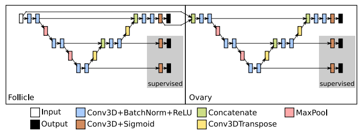
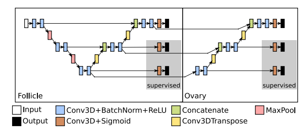
Our methods were then evaluated in respect to the effectiveness of ovary detection. If the 3D U-Net (with or without Deep Supervision) was trained in detecting ovaries directly (as by follicle detection), such an approach was significantly less successful than the baseline methods. A similar result was observed if our U-Net extensions were trained to detect follicles and ovaries simultaneously. Some results of these non-successful experiments are not reported. To detect the ovaries, we therefore utilised variations of both the U-Net extensions (i.e., EXT 1 and EXT 2) proposed in Section 3.3, whereas the network from the first stage was pretrained on the problem of ovarian follicle detection. A kind of Transfer Learning (see Section 3.5) was employed, because the weights of the network from the first stage were frozen, and were no longer adapted during the ovary detection training.

Table 5. Effectiveness of the proposed ovary detection methods trained and evaluated 50 times on the USOVA3D database. The minimum, maximum, mean and median of the overall algorithm’s score are presented over 50 runs. Entries are sorted with respect to the median value.

Method	min(${\mathit{\xi }}_{\mathit{alg}}$)	max(${\mathit{\xi }}_{\mathit{alg}}$)	mean(${\mathit{\xi }}_{\mathit{alg}}$) ± std(${\mathit{\xi }}_{\mathit{alg}}$)	median(${\mathit{\xi }}_{\mathit{alg}}$)
EXT 2 + DS (last)	63.0	76.0	71.7 ± 2.5	71.8
EXT 1 + DS (best)	62.1	76.2	70.3 ± 3.3	70.5
EXT 2 + DS (best)	60.0	74.9	69.1 ± 3.7	69.4
EXT 1 + DS (last)	53.1	77.7	68.9 ± 5.0	68.6
EXT 1 (best)	59.1	72.6	66.9 ± 3.1	67.0
EXT 1 (last)	53.7	71.8	64.7 ± 4.1	65.0
3D UNET (best)	56.8	72.8	64.2 ± 3.8	64.6
3D UNET + DS (best)	56.1	70.8	63.3 ± 3.4	63.3
EXT 2 (best)	54.0	68.9	62.2 ± 3.5	62.3
EXT 2 (last)	54.1	68.7	62.3 ± 3.3	62.3
3D UNET + DS (last)	50.0	63.0	58.0 ± 2.8	58.4
3D UNET (last)	43.8	69.8	56.8 ± 5.0	56.3

contains the results of ovary detection for both the proposed pretrained U-Net extensions (EXT 1 and EXT 2), with or without Deep Supervision (+DS). Each method was trained and evaluated 50 times on the USOVA3D database. Minimum, maximum, mean, and median are presented of the algorithm’s effectiveness over 50 runs. The ‘best’ designates that the CNN model with the lowest validation loss was selected, while the ‘last’ means that the model was picked in a particular run after the final training step.

In a similar way to the follicles, a comparison was also made with the state-of-the-art method SNET [11], USOVA3D baseline functions, and with the variability of both raters in ovary annotating. The results are gathered in

Table 6. Effectiveness of the proposed ovary detection methods compared to the state-of-the-art and inter-rater variability. The final score statistics are presented, together with the overall algorithm’s score on the USOVA3D database. Entries are sorted with respect to the overall score.

Method	median(${\mathit{\xi }}_{\mathit{vol}}$)	min(${\mathit{\xi }}_{\mathit{vol}}$)	max(${\mathit{\xi }}_{\mathit{vol}}$)	${\mathit{\xi }}_{\mathit{alg}}$
Rater 1 vs. rater 2	79.1	52.7	96.0	76.1
Rater 2 vs. rater 1	78.8	45.5	96.1	75.5
EXT 1 + DS (last)	79.9	51.6	91.5	77.7
EXT 1 + DS (best)	78.8	50.3	92.6	76.2
EXT 2 + DS (last)	80.9	52.1	93.4	76.0
EXT 2 + DS (best)	81.6	47.7	92.0	74.9
3D UNET (best)	75.8	47.7	88.4	72.8
EXT 1 (best)	75.9	48.9	93.3	72.6
2D UNET (baseline 2)	73.6	40.5	87.9	72.2
EXT 1 (last)	74.9	48.8	92.3	71.8
3D UNET + DS (best)	73.7	47.7	91.1	70.8
3D UNET (last)	71.4	42.5	92.2	69.8
SNET (best)	65.7	45.6	86.7	69.4
EXT 2 (best)	69.6	50.9	88.3	68.9
EXT 2 (last)	65.7	47.5	89.6	68.7
3D DWT (baseline 1)	72.5	18.3	87.1	63.3
3D UNET + DS (last)	59.3	42.2	92.6	63.0

. The more successful variants of the detection methods from this table were also evaluated using the Dice Similarity Coefficient and Jaccard Index (Sensitivity, Precision, and F1 score equals 1 for all ovary detection methods!). The mean and Standard Deviation of both metrics are presented in

Table 7. Effectiveness of the proposed ovary detection methods compared to the state-of-the-art and inter-rater variability. Presented are the mean and Standard Deviation of the Dice Similarity Coefficient (DSC) and Jaccard Index (JCI) on the USOVA3D database.

Method	DSC	JCI
Rater 1 vs. rater 2	0.880 ± 0.070	0.793 ± 0.111
Rater 2 vs. rater 1	0.880 ± 0.070	0.793 ± 0.111
EXT 1 + DS (last)	0.865 ± 0.088	0.771 ± 0.127
EXT 2 + DS (last)	0.852 ± 0.102	0.753 ± 0.143
3D UNET (best)	0.833 ± 0.112	0.728 ± 0.152
3D UNET + DS (best)	0.829 ± 0.108	0.722 ± 0.147
SNET (best)	0.802 ± 0.131	0.686 ± 0.162

.

Similarly as for follicles, we also calculated the effectiveness of better ovary detection methods at the level of all detected voxels, i.e., all metrics were calculated across all properly segmented voxels and not at the level of the entire ovary. The results are gathered in

Table 8. Effectiveness of the proposed ovary detection methods compared to the state-of-the-art and inter-rater variability, calculated on ‘voxel level’. Presented are the mean and Standard Deviation of Sensitivity or Recall (S), Precision (P), Dice Similarity Coefficient (DSC), Jaccard Index (JCI), and the Accuracy (ACC) on the USOVA3D database.

Method	S	P	DSC	JCI	ACC
Rater 1 vs. rater 2	0.936 ± 0.066	0.844 ± 0.126	0.880 ± 0.070	0.793 ± 0.111	0.930 ± 0.056
Rater 2 vs. rater 1	0.844 ± 0.126	0.936 ± 0.066	0.880 ± 0.070	0.793 ± 0.111	0.930 ± 0.056
EXT 1 + DS (last)	0.844 ± 0.128	0.906 ± 0.098	0.865 ± 0.088	0.771 ± 0.127	0.924 ± 0.065
EXT 2 + DS (last)	0.853 ± 0.145	0.870 ± 0.102	0.852 ± 0.102	0.753 ± 0.143	0.920 ± 0.059
3D UNET + DS (best)	0.813 ± 0.165	0.894 ± 0.120	0.833 ± 0.112	0.728 ± 0.152	0.909 ± 0.072
3D UNET (best)	0.805 ± 0.177	0.902 ± 0.114	0.829 ± 0.108	0.722 ± 0.147	0.913 ± 0.059
SNET (best)	0.802 ± 0.169	0.823 ± 0.124	0.802 ± 0.131	0.686 ± 0.162	0.899 ± 0.054

.

5. Discussion

Training (Convolutional) Neural Networks is, to some extent, a stochastic process. With constant input data, the transformation function that the CNN will learn also depends on the type of chosen optimisation algorithm, and the procedure by which synaptic weights are initialised. Based on a variety of experiments and studies, the research community has developed recommendations for selecting the more appropriate optimisation and weight initialisation procedures [23]. We followed these guidelines in this study as well. Even if the optimisation function and the weight initialisation procedure are fixed, as they were in this study, the CNN training is still stochastic. The reason is that synaptic weights are set initially to random values determined by some initialisation procedure. We argue that a new CNN is established after each repetition of training, whereas such CNN will, of course, implement a novel transformation function. The latter does not apply only in the exceptional case when the synaptic weights would be initialised to fixed values, thus obtaining an identical CNN after every training. However, the stochastic procedure for synaptic weights’ initialisation is employed commonly in practice (also in this research).

It is a standard convention in reporting the effectiveness of learning-based approaches that only a single best result is presented obtained with the selected CNN architecture. Unfortunately, such compact presentation also has drawbacks, as it is not evident whether the improvement in detection performance was only due to the stochasticity of weight initialisation, or whether it is really a methodological refinement of detection. For the reasons described, the training of our detection methods was repeated 50 times in this study. Various statistics for these 50 training runs, such as minimum, maximum, expected average and median effectiveness, were then summarised in the results (see Table 1 and Table 5). By comparison with the state-of-the-art, only the results of the best runs (models) were indeed incorporated in Table 2 and Table 6, but, in this discussion, we will evaluate the results more critically.

To begin with, it should be stressed that a kind of ablation study [24] was conducted in this article. Namely, we monitored the performance of our detection ‘system’ by removing/adding certain components, to understand the contribution of the component to the overall system. Let us focus on the follicles first. We noticed that the effectiveness of the original 3D U-Net (3D UNET) was in the range of results of the 2D UNET baseline method. The results have improved remarkably with the incorporation of Deep Supervision into 3D UNET (see Figure 3), which undoubtedly indicates the positive influence of this component on the follicle detection. With the proposed EXT1 and EXT 2 extensions, we were not able to improve the statistically significant the results of the ‘3D UNET + DS (last)’ method. The ‘3D UNET + DS (last)’ and ‘EXT 2 + DS (last)’ methods do not differ statistically significantly (Wilcoxon rank sum test at 5% significance level) based on 50 runs. However, it is also true that, by using our proposed methods, we obtained maximum overall algorithm’s scores higher than the ‘3D UNET + DS (last)’ method. On the other hand, the effectiveness of all the other follicle and ovary detection methods, from Table 1 and Table 5, trained and evaluated 50 times on the USOVA3D database, do differ statistically significantly (the same Wilcoxon test was applied).

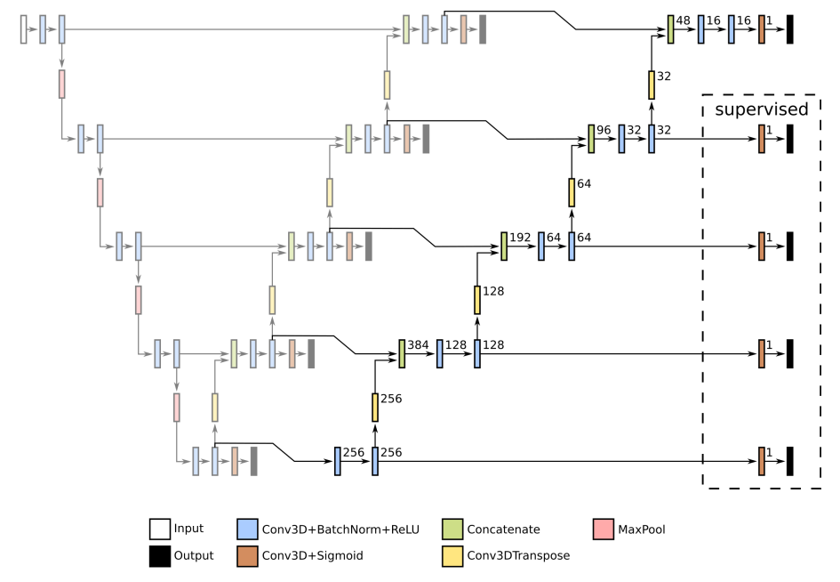
More consideration is needed by the ovary detection. In this work, we have expanded the original 3D U-Net once by duplicating the entire architecture (EXT 1 extension), and the second time by duplicating the decoder components (EXT 2 extension), as detailed in Section 3.3. The EXT 2 extension hardly improved the 3D UNET results, while the application of EXT 1 contributed on average up to a 2.7 higher overall algorithm score. The introduction of Deep Supervision in EXT 1 and EXT 2 also improved the results notably in the case of the ovaries. The average overall score increased at best by 6.1 (EXT 1) and 7.5 (EXT 2) respectively, simultaneously increasing training stability (see Mean and Standard Deviation in Table 5). A similar trend was observed for the median of the overall algorithm score. It should be noted that the mere integration of Deep Supervision into the original 3D U-Net has practically not improved the effectiveness of ovary detection.

An additional comment is needed when assessing the results using the best models on the validation set (denoted ‘best’), or the models after the last training step (‘last’), respectively. One would expect that, if a model is effective on a validation set, it will also be effective on a testing set, and vice versa. However, a certain inconsistency was noticed in Section 4. The reason is sought in the small USOVA3D database for which the testing set was determined manually without serious analysis [7]. The training set (with the validation set as part of it) does not summarise/reflect the statistics of the data in the testing set credibly, and, as a consequence, there were oscillations in performance by the ‘best’ and ‘last’ models.

Let us analyse the effectiveness of follicle and ovary detection using our proposed methods in this sequel. For follicle detection, it pointed out that the effectiveness of the 3D DWT baseline function was surpassed with the best runs of the ‘3D UNET + DS’ method and our proposed methods (see Table 2). As mentioned earlier, it can be misleading to observe only the results of the best training run. From Table 1 it can be noticed that the median of the ‘3D UNET + DS (last)’ and ‘EXT 2 + DS (last)’ methods are almost equal to the result of the 3D DWT baseline function. Based on the median and mean values, we concluded that a result better or equal to the USOVA3D baseline result would be got from every other run of these two methods. The latter undoubtedly confirms that our proposed method also improved the successfulness of the 3D DWT baseline function, and that the higher overall algorithm score was not merely due to the different initialisations of the CNN models. A similar conclusion can be drawn for our 3D ovary detection methods. The obtained results with the best runs of our approaches were at least in the rank of the better 2D UNET baseline function, or the baseline results were exceeded in most cases, respectively. When using both U-Net extensions with integrated Deep Supervision, the results of the best runs were alongside the inter-rater variability, while, in the case of the ‘EXT 1 + DS’ method, this variability was even exceeded. The mean and median statistics in Table 5 are more conclusive, which first reveal that, so far, the best 2D UNET (baseline) method was surpassed by both the ‘EXT 1 + DS’ and ‘EXT 2 + DS’ methods, and, at the same time, our proposed methods are still behind the accuracy of the raters. We notice in Table 6 that the inter-rater variability for the ovaries is importantly higher than for the follicles (i.e., lower ${\xi }_{alg}$ for ovaries than for follicles). This discrepancy in the raters’ annotations (labels) certainly affects the CNN models’ training with greater instability, thereby influencing the variation of the obtained results and their scatter (e.g., higher Standard Deviation). Let us emphasise once again that the labels of both raters were considered equally in the training.

Adding noise to training data is one of regularisation techniques that reduces the possibility of CNN overfitting [23]. Based on the Dice Similarity Coefficient calculated between both raters, we ascertained that the raters annotated the same ovarian ultrasound volume to some extent differently. Nevertheless, we passed both non-identical annotations for the same structure (i.e., for ovary or follicle) into the training, which, of course, introduced some noise into the data, but at the same time prevented the CNN from overfitting. It should also be emphasised that the ultrasound is a rather demanding modality, which is reflected in the subjective interpretation of the imaging material. Particularly pressing is the accurate determination of object boundaries (e.g., for ovaries and follicles), which are often inexpressive and jagged. The complexity of interpreting ultrasound data from the USOVA3D database is, thus, reflected in the higher inter-observer variability (e.g., DSC and JCI coefficients much lower than 1).

In our study, we chose S-Net [11], which is also based on the U-Net architecture, as a state-of-the-art for a comparison with our methods. Mathur et al. have shown in [11] that S-Net is currently the most effective follicle and ovary detection method. The latter was substantiated by 0.93 mean Sensitivity and by 0.92 (ovary) and 0.87 (follicle) mean Dice Similarity Coefficient (DSC) by detection, respectively. All metrics were calculated on 20 testing ovarian ultrasound volumes from their private database. To the best of our knowledge, their testing data and the code of S-Net are not publicly available, therefore, we implemented this method by ourselves, and tested it on the public USOVA3D database. The obtained results were evaluated both with our evaluation protocol and with the usual metrics (i.e., DSC, Jaccard index). It pointed out that our proposed ‘EXT 1 + DS’ and ‘EXT 2 + DS’ methods outperformed S-Net in virtually all metrics, both in follicle and ovary detection (see Table 2, Table 3, Table 6 and Table 7). Besides, we note that the ranking of detection methods based on our evaluation protocol or based on established metrics is consistent, whereat the advantage of our protocol being that we obtain a single effectiveness estimate for each method and, therefore, the methods do not need to be re-ranked according to each of the individual metrics. The following should be also emphasised when comparing effectiveness of our methods and S-Net. S-Net achieved very high mean sensitivity (0.93) and mean DSC (around 0.9) by detection on private testing data. For the public USOVA3D database, however, we observe that even inter-rater variability with 0.88 Sensitivity and Dice Similarity Coefficient of 0.88 (ovary) or 0.86 (follicles) is far behind the S-Net results. The latter indicates undoubtedly that USOVA3D is an extremely challenging database.

In our opinion, a direct comparison of the calculated effectiveness metrics for our methods with the effectiveness metrics of similar works is not relevant, as different research groups have evaluated their solutions (some were designed for 2D ultrasound data) on their private ovarian ultrasound data. The problem of the large variation in the algorithm’s effectiveness metrics, calculated on different data, was, in this study, demonstrated above in the case of the state-of-the-art S-Net method. Cigale et al. [9] compared in detail their 3D DWT detection method with selected advanced algorithms (including the SonoAVC algorithm integrated into General Electric ultrasound devices) on the same, i.e., today publicly available ovarian ultrasound data (at that time the USOVA3D database was not yet published). They demonstrated the superiority of their method by all criteria. This 3D DWT method was then added to the USOVA3D database as a baseline function 1. In this study, however, we proved experimentally that our proposed solutions surpassed the 3D DWT method in respect to the effectiveness. Based on all the results and analyses, our methods can also be considered the state-of-the-art in the field of Ovary and follicle detection.

Our study is not a clinical study, so information about clinically acceptable detection errors was not available. The comparison was, therefore, made with an inter-observer variability. The DSC coefficient was lower by less than 2% and the JCI index was lower by less than 3% in respect to the inter-observer variability (i.e., an estimate of detection accuracy that we can expect from experts) when detecting ovaries with our best ‘EXT 1 + DS’ method. In the detection of follicles, however, Sensitivity was lower by about 8%, the DSC coefficient by about 6% and the JCI index by about 7% in respect to the inter-observer variability. In summary, our best methods are, for ovary detection, in the range of the experts’ accuracy, while for follicle detection, we are still behind the experts, and, therefore, it would be necessary to verify the results manually in the clinical practice.

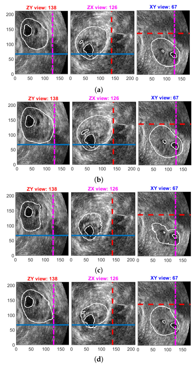
Figure 8 depicts some typical qualitative results for the better compared methods. Computer detected follicles and ovary are superimposed on the selected cross-sections of ovarian ultrasound volume. The difficulty of detection in the USOVA3D database can be seen clearly, as the edges of the follicles and ovary are very indistinct. Annotations of rater 1 for this volume and these cross-sections are shown in Figure 1.

Let us also consider the capacity of our CNN models. The original 3D U-Net has a little over 4.82 Million (M) of free parameters, while this number increased by 484 when the Deep Supervision was integrated. Both 3D U-Net extensions were designed primarily to detect the ovaries, however, they were also applied successfully for follicle detection. The EXT 1 architecture has a total of 9.64 M parameters, of which 4.82 M parameters are frozen or fixed by Transfer Learning (if the case of ovary detection), respectively. The frozen parameters are for the first stage of the EXT 1 model. The proposed EXT 2 extension is more complex, as it has a total of 11.41 M parameters, whereas also 4.82 M parameters from the first stage are frozen or pretrained (by ovary detection), respectively. The integration of Deep Supervison in the 3D U-Net extensions contributed an additional 968 parameters, of which 484 were trainable (by ovary detection). In contrast, although 2D UNET has a total of 31.13 M parameters, which is almost 3 times more than our proposed methods, its effectiveness of follicle and ovary detection is remarkably inferior to our methods. Our deep models were indeed trained on a small number of volumes (16) as there are no more training data available in the USOVA3D database. The lack of data was mitigated by meaningful preprocessing and the use of augmentation. The fact that we train our CNN models of segmentation, where each output voxel represents its own training sample, also contributed to the successful training of our models. The number of voxels in our volumes is, of course, extremely large. (It is also true that samples are not completely independent.) We did not diagnose the overfitting problem when training our CNNs by USOVA3D data.

CNN training is computationally demanding. An exhaustive experimentation with 50 repetitions of CNN models’ training was performed by using the HPC RIVR MAISTER powerful public supercomputer in Maribor, Slovenia (https://www.hpc-rivr.si, accessed on 1 January 2022). Six dual-processor compute nodes, each with 4 additional Nvidia Tesla V100 Graphics Processing Units, GPU (each GPU had 32 GB of RAM), with a total of 122,952 cores, were utilised on this supercomputer. Follicle detection training took about 3 s per step, or about 70 s per epoch. On the other hand, the EXT 1 and EXT 2 extensions, developed primarily for the ovary detection, took up to 5 s for the training step and about 120 s per epoch, respectively. The trained network conducted an inference in around 9 s per volume, which also includes all volume resizing, and storing the result on the secondary memory.

6. Conclusions

The main intention of this paper was to introduce efficient 3D object detection algorithms, aimed primarily to detect follicles and ovaries in ultrasound volumes. We took a learning-based design approach, relying on the established U-Net architecture, and upgrading it in this research. Two methods for indirect or two-stage object detection were developed respectively, namely, in the first solution the entire U-Net architecture was duplicated, while, in the second solution, just certain parts of the U-Net model decoder were replicated. The first stage of such CNN introduces a kind of prior knowledge into the detection process, as it directs the ‘second stage’ to that part of the 3D space (volume) where the searched object is more likely to be located. Deep Supervision was integrated into both CNNs as well, which had a positive effect on the training of the lower layers of the Neural Network. The proposed methods were verified by the detection of follicles and ovaries in ultrasound volumes. The methods were trained end-to-end by follicle detection, while an idea of Transfer Learning was utilised by ovary detection. The latter means that the ‘first stage’ of the CNN was trained separately on the problem of follicle detection, and, afterwards, the trained ‘first stage’ was, by Transfer Learning, employed by training the ‘second stage’ to detect ovaries.

The follicle detection results pointed out that our proposed U-Net extensions did not statistically significantly improve the results of the with Deep Supervision integrated 3D U-Net. However, we obtained higher effectiveness than 3D U-Net (+ Deep Supervision) by some repetitions of our CNNs’ training. On the other hand, the superiority of our proposed methods was indisputable in the detection of ovaries. The results pointed out up to 7.6% more accurate detection compared to the up-to-date automated ovary detection methods. Our two-stage CNNs estimated follicles only slightly worse than the raters, while our methods estimated the ovaries with almost the same accuracy as the raters. We verified by quantitative metrics that our proposed methods, both in the case of follicle and ovary detection, are more effective than the USOVA3D baseline functions and the state-of-the-art method S-Net [11] on the very challenging USOVA3D testing data.

We demonstrated that the improvements are not only due to the random initialisation of the CNN models, but that, by using the proposed modifications of the U-Net architecture, the follicles and ovaries were detected more accurately in a systematic way. By analysing 50 repetitions of training (and testing) of our CNNs statistically, we proved that the training is stable, and that in practically every other repetition the CNN is constructed, which is more efficient than the most accurate methods for detecting follicles and ovaries so far. In addition, it was substantiated that, despite using the small USOVA3D database, the detection algorithms can be trained quite successfully and without any data overfitting. A convergence was reached in a reasonable number of training steps.

Let us conclude this paper with some future work directions. One of the succeeding researches will be focused on applying and transferring our solutions to other problem domains. The aim will be to demonstrate that only minimal interventions are needed in our proposed detection algorithms. In the field of Ovarian Ultrasound Volumes’ Processing, we will upgrade our solutions further, in order to detect ovaries accurately in just one pass, without adding prior knowledge about follicles. Special attention will be paid to the augmentation of the small USOVA3D training set. Finally, we recommend that the statistical assessment of repetitive training and testing becomes the rule when also reporting results in the field of CNN-based approaches.

References

1. Vlaisavljević, V.; Knez, J. Chapter Ultrasound in Human Reproduction. In Donald School Textbook of Ultrasound in Obstetrics & Gynecology; Jaypee Brothers Medical Publishers: New Delhi, India, 2018. [Google Scholar] [CrossRef]
2. Gore, M.A.; Nayudu, P.L.; Valisavljević, V. Prediction of ovarian cycle outcome by follicular characteristics, stage 1. Hum. Reprod. 1995, 10, 2313–2319. [Google Scholar] [CrossRef] [PubMed]
3. Kelsey, T.; Dodwell, S.; Wilkinson, G.; Greve, T.; Andersen, C.; Anderson, R.; Hamish, W.; Wallace, B. Ovarian Volume throughout Life: A Validated Normative Model. PLoS ONE 2013, 8, e71465. [Google Scholar] [CrossRef] [PubMed] [Green Version]
4. Saleh, A.; Al-Saygh, F.; Abushama, M.; Ahmed, B. The Role of Three-Dimensional Ultrasound in Gynecology. Res. Women’s Health 2019, 1, 4. [Google Scholar] [CrossRef] [Green Version]
5. Potočnik, B.; Cigale, B.; Zazula, D. Computerized detection and recognition of follicles in ovarian ultrasound images: A review. Med. Biol. Eng. Comput. 2012, 50, 1201–1212. [Google Scholar] [CrossRef] [PubMed]
6. Noble, J.; Boukerroui, D. Ultrasound image segmentation: A survey. IEEE Trans. Med. Imaging 2006, 25, 987–1010. [Google Scholar] [CrossRef] [PubMed] [Green Version]
7. Potočnik, B.; Munda, J.; Reljić, M.; Rakič, K.; Knez, J.; Vlaisavljević, V.; Sedej, G.; Cigale, B.; Holobar, A.; Zazula, D. Public database for validation of follicle detection algorithms on 3D ultrasound images of ovaries. Comput. Methods Programs Biomed. 2020, 196, 105621. [Google Scholar] [CrossRef] [PubMed]
8. Deutch, T.D.; Joergner, I.; Matson, D.O.; Oehninger, S.; Bocca, S.; Hoenigmann, D.; Abuhamad, A. Automated assessment of ovarian follicles using a novel three-dimensional ultrasound software. Fertil. Steril. 2009, 92, 1562–1568. [Google Scholar] [CrossRef] [PubMed]
9. Cigale, B.; Zazula, D. Directional 3D Wavelet Transform Based on Gaussian Mixtures for the Analysis of 3D Ultrasound Ovarian Volumes. IEEE Trans. Pattern. Analy. Mach. Intel. 2019, 41, 64–77. [Google Scholar] [CrossRef] [PubMed]
10. Li, H.; Fang, J.; Liu, S.; Liang, X.; Yang, X.; Mai, Z.; Van, M.; Wang, T.; Chen, Z.; Ni, D. CR-Unet: A Composite Network for Ovary and Follicle Segmentation in Ultrasound Images. IEEE J. Biomed. Health Inf. 2020, 24, 974–983. [Google Scholar] [CrossRef] [PubMed]
11. Mathur, P.; Kakwani, K.; Diplav; Kudavelly, S.; Ramaraju, G.A. Deep Learning based Quantification of Ovary and Follicles using 3D Transvaginal Ultrasound in Assisted Reproduction. In Proceedings of the 2020 42nd Annual International Conference of the IEEE Engineering in Medicine & Biology Society (EMBC), Montreal, QC, Canada, 20–24 July 2020; pp. 2109–2112. [Google Scholar] [CrossRef]
12. Marques, S.A.C. Ovarian Structures Segmentation using a Neural Network Approach. Master’s Thesis, Faculdade de engenharia da universidade do Porto, Porto, Portugal, 2019. [Google Scholar]
13. Singh, S.P.; Wang, L.; Gupta, S.; Goli, H.; Padmanabhan, P.; Gulyas, B. 3D Deep Learning on Medical Images: A Review. Sensors 2020, 20, 5097. [Google Scholar] [CrossRef] [PubMed]
14. Getao, D.; Xu, C.; Jimin, L.; Xueli, C.; Yonghua, Z. Medical Image Segmentation based on U-Net: A Review. J. Imaging Sci. Tech. 2020, 64, 20508-1–20508-12. [Google Scholar] [CrossRef]
15. Ronneberger, O.; Fischer, P.; Brox, T. U-Net: Convolutional Networks for Biomedical Image Segmentation. In Proceedings of the Medical Image Computing and Computer-Assisted Intervention—MICCAI 2015, Munich, Germany, 5–9 October 2015; Volume III, pp. 234–241. [Google Scholar]
16. Lee, C.Y.; Xie, S.; Gallagher, P.; Zhang, Z.; Tu, Z. Deeply-supervised nets. In Proceedings of the Eighteenth International Conference on Artificial Intelligence and Statistics, San Diego, CA, USA, 9–12 May 2015; Volume 38, pp. 562–570. [Google Scholar]
17. Çiçek, Ö.; Abdulkadir, A.; Lienkamp, S.; Brox, T.; Ronneberger, O. 3D U-Net: Learning Dense Volumetric Segmentation from Sparse Annotation. In Proceedings of the Medical Image Computing and Computer-Assisted Intervention—MICCAI 2016, Athens, Greece, 17–21 October 2016; pp. 424–432. [Google Scholar]
18. Arrastia, L.L.; Heilenkötter, N.; Baguer, D.O.; Hauberg-Lotte, L.; Boskamp, T.; Hetzer, S.; Duschner, N.; Schaller, J.; Maass, P. Deeply supervised UNet for semantic segmentation to assist dermatopathological assessment of basal cell carcinoma. J. Imaging 2021, 7, 71. [Google Scholar] [CrossRef] [PubMed]
19. Rajalakshmi, N.R.; Vidhyapriya, R.; Elango, N.; Ramesh, N. Deeply supervised U-Net for mass segmentation in digital mammograms. Int. J. Imag. Sys. Technol. 2021, 31, 59–71. [Google Scholar] [CrossRef]
20. Tan, C.; Sun, F.; Kong, T.; Zhang, W.; Yang, C.; Liu, C. A Survey on Deep Transfer Learning. In Proceedings of the Artificial Neural Networks and Machine Learning—ICANN 2018 27th International Conference on Artificial Neural Networks, Rhodes, Greece, 4–7 October 2018; pp. 270–279. [Google Scholar] [CrossRef] [Green Version]
21. Zhuang, F.; Qi, Z.; Duan, K.; Xi, D.; Zhu, Y.; Zhu, H.; Xiong, H.; He, Q. A Comprehensive Survey on Transfer Learning. Proc. IEEE 2021, 109, 43–76. [Google Scholar] [CrossRef]
22. Kingma, D.P.; Ba, J.L. Adam: A method for stochastic optimization. In Proceedings of the 3rd International Conference on Learning Representations—ICLR 2015, San Diego, CA, USA, 7–9 May 2015. [Google Scholar]
23. Goodfellow, I.; Bengio, Y.; Courville, A. Deep Learning; MIT Press: Cambridge, MA, USA, 2017. [Google Scholar]
24. Zhang, R.; Chung, A.C.S. MedQ: Lossless ultra-low-bit neural network quantization for medical image segmentation. Med. Image Anal. 2021, 73, 102200. [Google Scholar] [CrossRef] [PubMed]
Figure 1. Sample ultrasound volume from the USOVA3D database: (a) 2D views of an annotated ovary (ochre) with follicles (coloured) superimposed on the selected cross-sections: ZY plane (left), ZX plane (middle) and XY plane (right); (b) A 3D view of the cross-sections, shown in (a), through volume with annotated follicles; and (c) The 3D view of the corresponding ovary.
Applsci 12 01246 g001
Figure 2. Basic U-Net architecture with three multi-scale layers.
Applsci 12 01246 g002
Figure 3. Three multi-scale layer U-Net with Deep Supervision. Additional outputs are introduced at lower scales.
Applsci 12 01246 g003
Figure 4. Example of the first proposed U-Net extension, EXT 1—two consecutive U-Nets: The segmentation map of the first stage is concatenated with the input and passed as the input to the second stage. The first stage detects follicles, while the second stage identifies the ovary. Deep Supervision outputs are shown in a grey box.
Applsci 12 01246 g004
Figure 5. Example of the second proposed U-Net extension, EXT 2—U-Net with a series of additional decoders. The first stage detects follicles, while the additional decoders in the second stage identify the ovary. Deep Supervision outputs are shown in a grey box.
Applsci 12 01246 g005
Figure 6. Basic U-Net architecture with five scales, as used in our experiments. In front of each scale on the left are depicted the spatial dimensions of the feature maps at that scale. Next to each individual operation block on the arrow is marked the number of output channels for that block.
Applsci 12 01246 g006
Figure 7. New layers of the second U-Net extension (EXT 2) with five scales, as used in our experiments. These layers (on the right) are connected with the basic U-Net (on the left), which is depicted without annotations. See Figure 6 for an explanation of the basic U-Net and used denotations.
Applsci 12 01246 g007
Figure 8. Qualitative results for the better compared methods. Detected follicles and ovary are superimposed on the selected cross-sections: (a) ‘EXT 1 + DS (best)’ method; (b) ‘EXT 2 + DS (last)’ method; (c) ‘SNET (best)’ method; (d) ‘3D UNET + DS (best)’ method. Rater’s annotations are shown in Figure 1.
Applsci 12 01246 g008