Abstract
Power quality disturbance (PQD) is an influential situation that significantly declines the reliability of electrical distribution systems. Therefore, PQD classification is an important process for preventing system reliability degradation. This paper introduces a novel algorithm called “adaptive salp swarm algorithm (SSA)” as an optimal feature selection algorithm for PQD classification. Feature extraction and classifier of the proposed classification system were based on the discrete wavelet and the probabilistic neural network, respectively. The classification was focused on the 13 types of power quality signals. The optimal number of selected features for the proposed classification system was firstly determined. Then, it demonstrated that the optimally selected features resulted in the highest classification accuracy of 98.77%. High performance of the proposed classification system in the noisy environment, as well as based on the real dataset was also verified. Furthermore, the proposed SSA indicates a very high convergence rate compared to other well-known algorithms. A comparison of the proposed classification system’s performance to existing works was also carried out, revealing that the proposed system’s accuracy is on a high-range scale. Hence, the adaptive SSA becomes another efficient optimal feature selection algorithm for PQD classification.
1. Introduction
Electricity is widely regarded as a critical factor in economic growth, as increased usage is required to serve a diverse range of load types, including industrial, commercial, and residential customers [1,2,3,4]. Renewable energy sources have been widely used to improve the capacity of electrical generation, particularly in the last few decades [5,6,7]. Power quality disturbance (PQD) has been a highly concerning problem in power systems since it can essentially degrade the system’s performance. In particular, this problem becomes more serious in the system having several non-linear loads and renewable energy distributed generators since these factors typically have high uncertainty [8]. Typically, PQD can occur in different forms, i.e., voltage sag, swell, interruption, harmonic, spike, transient, notch, or their combination [9,10,11]. To prevent the damage to the power system due to PQD, several tools have been proposed to identify the type of disturbances [12,13,14,15,16]. Signal processing is the main technique used in PQD classification since it is capable of accurately characterizing the type of signals [17].
Feature extraction is extensively known as an effective signal processing technique to classify the type of PQDs through their features [18,19,20,21,22,23]. In the literature, there were many signal processing methods performed in the feature extraction. Fourier transform (FT) is the famous frequency domain signal analysis that can extract the spectrum of stationary signals at specific frequencies. However, the FT has low performance in extracting the feature of non-stationary signals due to its fixed window function [24]. Short time Fourier transform (STFT) is a reform of FT in which the time-frequency window of temporary transient signal localization is improved from FT. Later on, the discrete wavelet transform (DWT) was developed by improving the fixed resolution issue of the STFT. Therefore, this extraction method is capable of providing a short window function at high frequency phases while maintaining a long window function at low frequency phases [25].
Since the feature extraction based signal processing can distinguish only the characteristics of signals, the additional tool called classifier has been widely used to increasingly improve the accuracy of PQD classification by classifying the type of PQD signals [26,27,28]. In previous studies, several techniques have been performed as a classifier for PQD classification, for example, artificial neural networks (ANN), support vector machines (SVM), expert systems, fuzzy logic [29,30,31,32,33,34,35]. In particular, many previous studies claimed that the ANNs have a competently higher potential for classifying PQD than the other classifier tools [36,37,38]. Furthermore, the feature selection process has extensively been used in PQD classification research, aiming to improve the performance of the classification system [39,40,41]. The main goal of this process is to optimally select the appropriate data of feature extracting data, so that the processing time and classification accuracy can be improved by eliminating unnecessary data [40,41].
Many research works in the literature have implemented feature selection techniques for PQD classification, demonstrating that this tool can significantly improve classification accuracy, as following detail. In 2009, B. Biswal et al. proposed the optimal feature selection algorithm for PQD classification using the adaptive particle swarm optimization (PSO) method, while the ST was used as feature extraction and the fuzzy C-means was performed as a classifier. It was found that this system could provide a classification accuracy of 96.33% [42]. In 2013, the PQD classification system using the k-means with an Apriori algorithm as optimal feature selection and WT as feature extraction was introduced, while the least squares support vector machine (LS-SVM) was performed as a classifier to classify five PQD signals [43]. It showed that 98.88% classification accuracy can be obtained. Next, R. Ahila et al. presented a combination of PSO algorithm and DWT in PQD classification based on the extreme learning machine (ELM) classifier, it was demonstrated this system could achieve 97.60% classification accuracy [44]. In 2016, A. A. Abdoos et al. proposed the PQD classification system that uses the sequential forward selection algorithm for optimal features selection, ST with variational mode decomposition (VMD) for feature extraction, and SVM as a classifier. It was shown that this system could reach a classification accuracy of up to 99.66% for nine PQD signal types [21]. In 2017, T. Chakravorti et al. showed that the PQD classification with the Fischer linear discriminant analysis algorithm for optimal feature selection, VMD as feature extraction, and reduced kernel extreme learning machine (RKELM) as a classifier could provide a classification accuracy of 98.82% [45]. Recently, Lei Fuei et al. performed the permutation entropy and the Fisher score algorithm for finding the optimal features of PQD classification using VMD for feature extraction, and one-versus-rest support vector machine (OVR-SVM) for a classifier [46]. Classification accuracy of 97.6% was demonstrated.
From the literature surveys, it shows that numerous recent works focus mainly on developing the ability of feature selection to improve the performance of PQD classification system. We also noticed that this process strongly influences the signal’s features before entering the classifier. Rather than state of the art in PQD classification, our hypothesis was the performance of the existing PQD classification system can be improved increasingly, especially system accuracy and convergence rate. Therefore, the contribution of this work is to introduce the PQD classification system based on a novel algorithm, namely, the adaptive salp swarm algorithm (SSA) as the feature selection algorithm. This new algorithm is supposed to reach a higher classification performance than the previous studies. The proposed approach was inspired by the fact that the SSA can efficiently find the solution of optimization problems within a short time due to its great exploration, which are typically the required properties in PQD classification. Another research gap was that, despite the high capability of SSA in solving many optimization problems in power systems, the use of this algorithm in power quality classification had not yet been reported. The proposed classification system performed DWT as feature extraction, while the probabilistic neural network (PNN) was used as the classifier. The verification of our proposed system was made based on the real dataset of distribution system. The performance of proposed classification system was compared to that of the previous PQD classification systems.
The rest of this paper is arranged as follows: A synthesis of power quality signals using mathematic equations under specific constraints is shown in Section 2. Section 3 describes the feature extraction process, while Section 4 explains the classifier based on a probabilistic neural network. Section 5 expresses the mechanism of the adaptive SSA as optimal feature selection. Then, Section 6 shows the simulation results including the related discussions. Finally, the results are concluded in Section 7.
2. Power Quality Disturbance Signals
In this research, the PQD signals were generated following the IEEE-1159 standard. We focused on 13 types of PQD signals consisting of 10 single types, which are pure sine, sag, swell, interruption, harmonic, impulsive transient, oscillatory transient, flicker, notch, and spike, and 3 combined signals including sag with harmonic, swell with harmonic, and interruption with harmonic. All signals were randomly generated within their constraints at 50 Hz, 1 p.u. of amplitude, 10 cycles, 2000 sampling points at 10 kHz. The mathematic equations and parameter constraints of all signals are shown in Table 1.

Table 1.
Power quality disturbance’s mathematical equations, adapted from: [9].
3. Feature Extraction
The overall process of PQD classification is shown in Figure 1. After the PQD signals generation, the signals were separated into training and testing data and passed through the feature extraction which is the process of creating the features of PQD signals. In this work, the signal’s characteristics were firstly extracted from the raw dataset of PQDs using the WT, as explained in Section 3.1. Then, the wavelet coefficients were obtained through the multi-resolution analysis (MRA), as detailed in Section 3.2. The procedure to create the feature vectors based on the their existing wavelet coefficients and statistical parameters is described in Section 3.3.
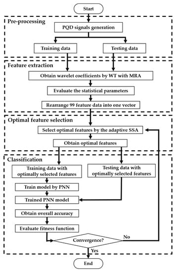
Figure 1.
PQD classification scheme.
3.1. Wavelet Transform
In the PQD classification research, several signal processing techniques have been used for characterizing the characteristics of signals, i.e., wavelet transform, DWT, S-transform, VMD, etc. [18,42,43,46,47]. In this work, we used the DWT for extracting the signal characteristics due mainly to its flexible time-scale and high conservation of information without reduced resolution [17,48]. This method has also been used extensively in many applications for power systems, such as fault detection and localization, classification of the shunt compensated transmission line, islanding detection technique, and PQD classification [48,49,50,51]. The DWT is transformed from the WT based on a discrete wavelet scales. The expression of DWT is given as following equation;
where the parameter indicates the frequency localization, is the time localization, represents the scaling parameter that repeats the length of wavelet as a function of , is the translation parameter, is the discrete point sequence of signal. The represents the mother wavelet based on the fourth-order Daubechies, since its suitability for PQD classification was claimed in several previous studies [52,53].
3.2. Multi-Resolution Analysis
The MRA is the process that uses the scaling function and orthogonal wavelet function to decompose and reconstruct signals at various resolution levels. This process benefits for filtering the propitious information of input signals, so the resulting signals are easier to be further implemented and require less execution and memory [22]. In this work, we used the MRA for decomposing the PQD signals before constructing the feature vectors. The procedure of MRA can be described as follows; the continuous-time PQD signals are passed through the filtering system that consists of low-pass (LP) and high-pass (HP) filters at different resolution levels. The high-frequency component having the first detail coefficient (D1) was obtained by HP filtering the down-sampling signal. Likewise, a low-frequency component having the first approximation coefficient signal (A1) is obtained by LP filtering the down-sampling signal. Afterwards, the output of A1 is decomposed before calculating the second detail coefficient (D2) and approximation coefficient (A2). This process was repeatedly operated until eight decomposition levels were achieved since it was confirmed in the previous study that this desired value is appropriate for extracting the characteristics of the PQD signals [53]. The feature vector of PQD signals, F(k), is then constructed from the obtained coefficients, as written in Equation (2)
3.3. Feature Vector Arrangement
After nine signal characteristics of PQD signals were obtained by the MRA process, the statistical parameters of signals were evaluated based on the signal’s characteristics. In this work, we focused on 11 statistical parameters including the energy (E), entropy (Ent), standard deviation (s), mean value (m), kurtosis (KT), skewness (SK), root-mean square (RMS), range (RG), log-energy entropy (LEnt), crest factor (CF), and form factor, as shown in Table 2. i, j = 1, 2, 3, …, l are the wavelet decomposition numbers at level l. N is the signal coefficient quantity in each decomposed data. X is the signal collected from eight detailed signals (D1, D2, …, D8) and one approximate signal (A8).
Table 2.
Equations for statistical parameter.
The feature vector of each statistical parameter was then constructed by the 11 detailed signals and one approximate signal, as shown in Table 3. It is shown that the overall features having 99 data are organized based on the type of statistical parameters.
Table 3.
Creation of feature vectors from statistical parameters, adapted from: [54].
Since the feature vectors calculated from the statistical parameters might have a large difference in scale, they have to be normalized before passing through the classifier, as given in Equation (3);
where is the normalized data, is the feature vectors, and are the feature vectors having the minimum and maximum value. Therefore, the overall feature set can be obtained using Equation (4).
4. Probabilistic Neural Network as a Classifier
In the PQD classification, the classifier is a process that classifies the power quality signal type. From the literature, many approaches have been performed as the classifier in power quality classification research [55,56,57]. PNN, which is one type of ANN, is a very well-known machine learning technique that has been extensively performed in several classification research [58]. The PNN uses the probabilistic model to operate the neural network for the pattern recognition [58]. Advantages of PNN include its high ability to achieve the results of non-linear learning algorithms with preserving high precision, as well as its simple implementation because the weights and network’s number of hidden layers are defined automatically by the network via the spread constant. PNN is also known as a powerful tool to solve various classification problems [59,60,61]. Our hypothesis was that the PNN could be highly appropriate for the proposed classification system according to its merits; thus, the PNN was used as classifier in this work. As shown in Figure 2, the PNN scheme contains the input and output layers separated by the hidden layer. Initial weight of each node is initialized automatically. The distribution value or probability density function is used to classify the input dataset. Then, the probability density function is used to determine the output hidden layers. The same probability as the category unit in which the model units contribute to a signal is addressed. A Gaussian based on the associated training dataset creates the test dataset. The neural network is supplied by the summation of these local estimates calculated in the relevant category unit.
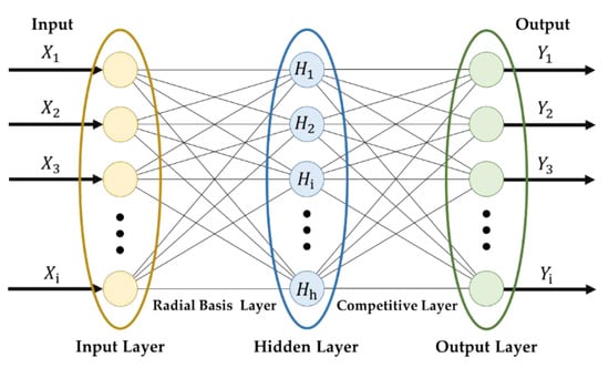
Figure 2.
PNN scheme.
According to the PQD classification scheme depicted in Figure 1, after the optimally selected features were obtained from feature selection, they were passed through the PNN-based classifier. The dataset was then trained and used for classifying the power quality signal types.
5. Proposed Adaptive Salp Swarm Algorithm for Optimal Feature Selection
As extensively demonstrated in several literature surveys, the optimal feature selection in PQD classification is a procedure that could significantly improve the performance of the classification system [42,43,44,45,46]. It is a process that selects the optimal features from feature extracting data before passing those features through the classifier. Accordingly, this process can efficiently eliminate the redundant features of extracting data, yielding better classification accuracy, as well as faster computational time. Referred to Figure 1, we used the feature selection process to optimally select features before passing through the PNN classifier. As mentioned in the introduction, there were plenty of previous studies that developed many optimization algorithms for optimal feature selection in PQD classification. Especially, it was claimed in many literature surveys that the swarm intelligence algorithm such as PSO, comprehensive learning PSO, modified PSO and SSA are effective for solving real-world applications [62,63]. However, we noticed that the SSA could be another capable algorithm for optimal feature selection since it has many required properties in PQD classification such as good convergence acceleration, accelerated process in getting high precise solution, great neighborhood search characteristic, simple implementation, reasonable calculating time, and a parameter tuning [64,65,66]. We used the SSA for optimal feature selection in our PQD classification system, and it was performed using the proposed adaptive techniques for ability improvement of this algorithm.
5.1. Salp Swarm Algorithm
In 2017, the SSA was proposed and claimed as another high-ability algorithm for solving optimization problems [64]. The SSA was introduced by simulating the swarming movement of salps. The advantages of this algorithm are their fewer control parameters, simple expression, qualitative global exploration, fast convergence rate, accelerated process in getting high precise solution, and small required data storage. The SSA is used extensively in many past optimization research [67,68,69,70]. We also noticed that its advantages are suitable for PQD classification. For this reason, we proposedly performed the SSA as an optimal feature selection algorithm in PQD classification. The mechanism of SSA is the salps moving in a chain pattern. The salp chain is made up of two salp groups: leader salps and follower salps. The leader, which is responsible for exploration of the food location, determines the direction of movement by taking the first position in front of the chain. The followers follow the leader and move after the leader movement. The expression of leader’s position is given in the following equation;
where is the leader position at j dimension. represents the food position. and are the upper and lower boundaries. and are the random numbers between 0 and 1. represents a movement of the leader toward the food, defined as the following equation;
where is the current iteration and is the maximum number of iterations. The position of followers can be updated using Newton’s law of motion, as shown in Equation (7);
where is the position of following salp of i-th follower in j dimension ( ≥ 2), is the acceleration value, is time, is an initial speed. Then, the position of followers can be updated using Equation (8).
5.2. Proposed Adaptive Salp Swarm Algorithm
In this work, we performed two approaches to improve the ability of SSA as the feature optimal selection algorithm. Section 5.2.1 describes the first approach to modifying salp movement behavior while searching for a food source, meanwhile Section 5.2.2 describes the adaptive technique to improve the performance of SSA.
5.2.1. Proposed Approaches for a Modification of Salp Movement
The salp movement for the SSA begins with the leader exploring the food position, while the followers move in a chain pattern. The leader’s position updates depending on the food location, which requires the calculated boundaries. This mechanism usually decreases the direct interaction between the leader and the food. The follower’s chain pattern depends only on the position of the leader. These mentioned behaviors of SSA sometimes cause a poor development between exploitation and exploration in case that the leader falls into the local optimum, which results in its low precision. Therefore, we propose a new parameter to control the convergence speed of a leader while searching for food, it is called “searching control parameter, ”. This proposed parameter is supposed to improve the balance between exploitation and exploration of SSA to avoid the local optimum. The is included in the conventional expressions for salp positioning of SSA, and then those equations can be rewritten as Equations (9) and (10).
In addition, we also proposedly adjust the moving direction of the leader to have wider spreading behavior through the parameter c1 of the leader’s movement of each iteration, as shown in Equation (11).
5.2.2. Proposed Adaptive Salp Swarm Algorithm
Since we noticed, from a literature review, that the main disadvantage of SSA is their local optima issue. Then, we propose the adaptive technique to solve this weakness of SSA by improving its development ability between exploitation and exploration. The idea of this proposed technique is to enlarge the searching space of the salp while finding the new salp’s position, which may possibly be located nearby. The procedure of the PQD classification using the adaptive SSA as the feature selection algorithm is described in following detail, while its pseudo code is illustrated in Figure 3.
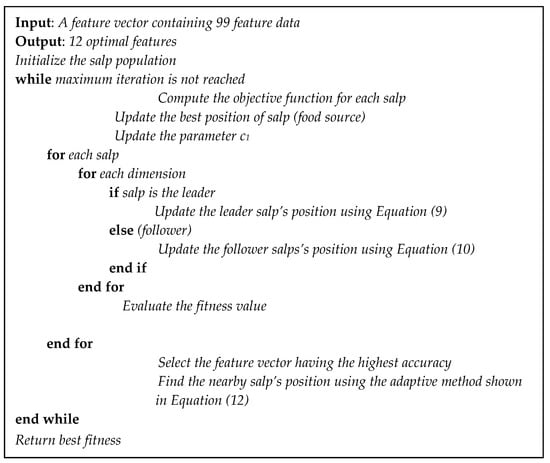
Figure 3.
Pseudocode of the proposed adaptive SSA.
Step 1: Initialize the number of salp population, dimension of the feature extracting data and iteration parameters;
Step 2: Create the feature vector randomly based on the setting upper and lower boundaries, defined dimension, and salp initialization;
Step 3: Pass the feature vector through the classifier. Calculate the percentage classification accuracy by a correctly classified signal types divided by the total test signals. Memorize the feature vector having the highest accuracy in the current population;
Step 4: Update the parameter c1 according to each iteration using Equation (11), and then randomly generate the parameters c2 and c3;
Step 5: Evaluate the leader’s position based on the parameters c1, c2, and c3 obtained from Step 4 using Equation (5). Then, the follower’s position based on the existing leader position is determined using Equation (8). Once all dimensions are built, calculate the accuracy;
Step 6: Perform the proposed adaptive technique, as the following detail. Select the feature vector having the highest accuracy at current iteration to enter the adaptive process. This process aims to further find the new position of salp nearby the current position which might has better accuracy than the existing one. At the each iteration of adaptive process, the adaptive coefficient value of the previous iteration, , is randomly generated for calculating the adaptive coefficient value of the current iteration, , with taking into account the initial weight, , and the final weight, , as expressed in Equation (12). The weight parameters developed in this work are used to determine the search space of the feature data in each iteration of adaptive process. is the current iteration of the adaptive method, is the maximum iteration number of the adaptive process. is the iteration number of SSA process. After that, the feature vector of the adaptive process, , is obtained based on the salp’s current position having the highest accuracy, , with taking into account the and the , as expressed in Equation (13). Where is the random feature vector between lower and upper boundaries of feature extracting vector, generated to indicate the data range of adaptive process compared to the ;
where is the feature dimension. The feature vector obtained from the adaptive process is passed through the PNN classifier, and then the classification accuracy is calculated;
Step 7: Repeat the adaptive process until the its maximum iteration is reached. Collect the feature vector of adaptive process indicating the highest classification accuracy;
Step 8: Compare the classification accuracy obtained from the adaptive process to that existed in iterations of SSA, then collect the feature vector that has the highest classification accuracy;
Step 9: Repeat Step 3 to 8 until the maximum number of iterations is reached. Obtain the optimal feature vectors.
6. Results and Discussion
In this section, the performance of the proposed classification system is shown and discussed based on the 13 types of power quality signals. The system feature extraction was based on the DWT, while the classifier was based on the PNN. The results were based on the SSA’s control parameters including number of salp = 10, iteration = 40, run 3 times, 20 independent runs, λ1 = 0.5, and λ2 = 0.1. MATLAB environment was performed in the simulations. The section is organized as follows: Section 6.1 investigates the optimal number of selected features for the proposed classification system. The accuracy of the PQD classification based on the proposed adaptive SSA is discussed in Section 6.2. The classification accuracy under a noisy situation is demonstrated in Section 6.3. The convergence property of the classification systems is indicated in Section 6.4. The simulations based on the real dataset are demonstrated in Section 6.5. Finally, Section 6.6 shows a performance comparison of the proposed classification system to the previous studies.
6.1. Optimal Number of Selected Features for the Proposed Classification System
Since the number of selected features obtained from the feature selection process typically has an impact on the classification accuracy, we firstly investigated the optimal number of selected features for our PQD classification. Table 4 shows the classification accuracy of various numbers of selected features, with the results based on the adaptive SSA. This table indicated that with over 5 selected features, higher precision than 1 to 4 selected features is obtained. In particular, the highest classification accuracy of 98.77% can be achieved with 12 optimally selected features. In addition, Table 5 shows further detail of classification accuracy at each iteration having different selected features by the adaptive SSA. It shows that the highest accuracy with the optimally selected features indicated is achieved at iteration 79. The results displayed in the next sections are based on these 12 optimal features.
Table 4.
Classification accuracy with different numbers of features selected.
Table 5.
Classification accuracy of each iteration having different selected features.
6.2. PQD Classification Accuracy Using the Adaptive SSA
To look closer into the mechanism of the adaptive SSA in PQD classification, Table 6 demonstrates the classification accuracy using the adaptive SSA and without feature optimal selection. The difference in performing different statistical parameters in classification was also taken into account. It is seen that using a single statistical parameter has poor capability in classification. Meanwhile, the classification accuracy improves when using a greater number of statistical parameters. This finding indicates that multiple statistical parameters are typically required to achieve high accuracy in PQD classification. The 94.38% accuracy was obtained for a case with all statistical parameters included excluding the optimal feature selection process. The highest accuracy was demonstrated for a case using 13 statistical parameters with the proposed adaptive SSA al optimal feature selection algorithm.
Table 6.
Classification accuracy using different statistical parameters.
6.3. Classification Pergormance under a Noisy Environment
A noisy condition is a situation that typically occurs in a practical distribution system. Therefore, the performance of the proposed classification system under a noisy environment was tested and compared to the conventional SSA, as well as the well-known methods, which are the conventional particle swarm optimization (PSO) and the Genetic algorithm (GA), as feature selection algorithms. The expression of these comparative algorithms was adopted from references [33,44,64]. The key parameters of PSO were set as follows; population size = 10, max inertia weight = 0.9, min inertia weight = 0.4, acceleration factor = 0.9, maximum number of iterations = 40, maximum needed number of runs = 20. The key parameters of GA were set as follows; population size = 10, max number of generations = 40, number of binary bits per design variable =10, crossover rate = 0.9, mutation rate = 0.1, transition probability = 0.01, maximum number of runs need to be = 20. Meanwhile, the key parameters of SSA were set similarly to the its adaptive. White noise with a signal-to-noise ratio of 10 to 50 dB were identically added to all power quality signal types. From Table 7, it is seen that the classification system based on the adaptive SSA optimal feature selection is qualitatively more resistant to noise than a system without an optimal feature selection, using conventional SSA, using PSO and using GA as optimal feature selection. Therefore, the proposed system could be efficiently operated in a noisy environment.
Table 7.
Accuracy of PQD classification under a noisy environment.
6.4. Convergence Rate
As mentioned earlier, one of the outstanding advantages of the SSA is its very fast convergence property. It is, therefore, necessary to examine the convergence profile of the proposed algorithm. In this work, we compared the convergence rate of our proposed system to the convergence rates of other well-known algorithms, such as PSO and GA. Figure 4 shows a comparison of the convergence rate of the PQD classification system using different algorithms for optimal feature selection, while the detail of accuracy and required iterations is summarized in Table 8. It was found that the system based on the adaptive SSA had the highest convergence rate to reach the classification accuracy of 98.77% at iteration 79. The conventional SSA can provide 96.85% accuracy at iteration 105. Meanwhile, the accuracy of 98.46% was reached by the PSO at iteration 80 and of 98.15% was reached by the GA at iteration 106. Then, the classification system using the adaptive SSA is not only able to provide very high accuracy, but it also has a rapid convergence rate.
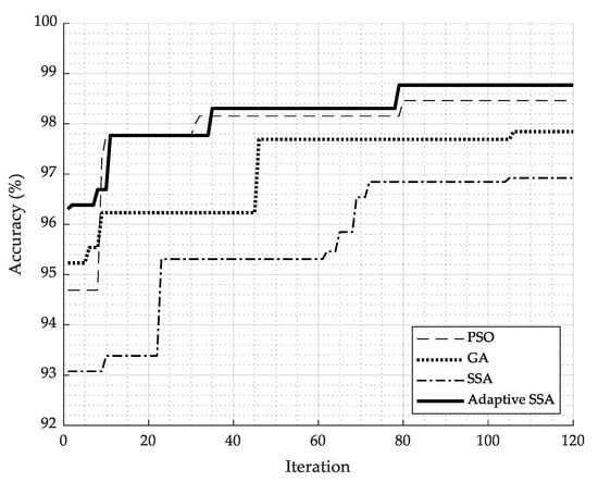
Figure 4.
Convergence rate of classification system using different feature selection algorithms.
Table 8.
Detail of classification performance using different feature selection algorithms.
6.5. Classification Performance Based on the Real Dataset
To validate the accuracy of the proposed classification system, it was tested using the real dataset of the practical distribution networkThe dataset was adopted from the PQube equipment, which is a tool used for real-time monitoring the power quality and electrical signal phenomena [71]. We focused on a case study of the distribution system located in Singapore, China, Sweden, and South Africa. Table 9 displays the classification system’s accuracy when using adaptive SSA as the optimal feature selection. It was found that the classification system proposed in this work provides 98.5% accuracy for identifying 5 types of power quality signals, which is consistent with that obtained by using the synthetic waveforms (98.8%).
Table 9.
Classification accuracy using the real dataset.
6.6. Comparison of Classification Performance to the Existing Works
To compare the performance of our proposed PQD classification to the other existing works, Table 10 shows a list of the accuracy of PQD classification appeared in the literature. Noted that accuracy of each mentioned system is adopted from those references. It is seen that the 98.77% classification accuracy of our proposed system is classified as very high value compared to the existing works. Additionally, our classification system can classify power quality signals of up to 13 different types, which is more than most research in this field. Furthermore, the classification system using the SSA as an optimal feature selection algorithm can quickly provide a solution. Hence, the classification system proposed in this work is another capable method for PQD classification and is appropriate for use in practical distribution systems.
Table 10.
Comparison of classification accuracy to the existing works.
7. Conclusions
In this work, we introduced a new algorithm called the adaptive SSA as a feature selection algorithm for PQD classification. The classification system’s feature extraction was based on the DWT and the classifier uses probabilistic neural network. The adaptive approaches were proposedly performed to enhance the ability of SSA for classification. It was found that the presented system indicated the best performance through 12 optimally selected features. The results showed that the highest accuracy in the classification of 13 types of signal power quality of 98.77% was achieved. Additionally, the proposed classification system can greatly operate in the noisy situation and the real dataset. The convergence rate of the system based on adaptive SSA was very high compared to the SSA, PSO, and GA. Considering the classification accuracy of previous studies reveals that the proposed classification system’s accuracy falls on a high-range scale, implying that it is capable of being another efficient PQD classification system.
Author Contributions
Conceptualization, S.C., A.S., and P.K.; data curation, S.C.; resources, P.K.; methodology, S.C., A.S., and P.K.; software, S.C.; formal analysis, S.C., A.S., P.F., P.S., and P.K.; investigation, P.K.; validation, S.C. and P.K.; writing—Original draft preparation, S.C.; writing—Review and editing, P.K.; supervision, P.K.; visualization, A.S., P.F., and P.S.; project administration, P.K.; funding acquisition, P.K. All authors have read and agreed to the published version of the manuscript.
Funding
This work was financially supported by the Provincial Electricity Authority (PEA).
Institutional Review Board Statement
Not applicable.
Informed Consent Statement
Not applicable.
Data Availability Statement
The data of real power quality signals presented in this study are openly available in http://map.pqube.com (accessed on 24 February 2021).
Conflicts of Interest
The authors declare no conflict of interest.
References
- Kandananond, K. Forecasting electricity demand in Thailand with an artificial neural network approach. Energies 2011, 4, 1246–1257. [Google Scholar] [CrossRef]
- Srithapon, C.; Ghosh, P.; Siritaratiwat, A.; Chatthaworn, R. Optimization of electric vehicle charging scheduling in urban village networks considering energy arbitrage and distribution cost. Energies 2020, 13, 349. [Google Scholar] [CrossRef]
- Khaboot, N.; Srithapon, C.; Siritaratiwat, A.; Khunkitti, P. Increasing benefits in high PV penetration distribution system by using battery enegy storage and capacitor placement based on salp swarm algorithm. Energies 2019, 12, 4817. [Google Scholar] [CrossRef]
- Srithapon, C.; Fuangfoo, P.; Ghosh, P.K.; Siritaratiwat, A.; Chatthaworn, R. Surrogate-Assisted multi-objective probabilistic optimal power flow for distribution network with photovoltaic generation and electric vehicles. IEEE Access 2021, 9, 34395–34414. [Google Scholar] [CrossRef]
- Boonluk, P.; Khunkitti, S.; Fuangfoo, P.; Siritaratiwat, A. Optimal siting and sizing of battery energy storage: Case study seventh feeder at Nakhon Phanom substation in Thailand. Energies 2021, 14, 1458. [Google Scholar] [CrossRef]
- Boonluk, P.; Siritaratiwat, A.; Fuangfoo, P.; Khunkitti, S. Optimal siting and sizing of battery energy storage systems for distribution network of distribution system operators. Batteries 2020, 6, 56. [Google Scholar] [CrossRef]
- Khaboot, N.; Chatthaworn, R.; Siritaratiwat, A.; Surawanitkun, C.; Khunkitti, P. Increasing PV penetration level in low voltage distribution system using optimal installation and operation of battery energy storage. Cogent Eng. 2019, 6, 1641911. [Google Scholar] [CrossRef]
- Morsi, W.G.; El-Hawary, M.E. Power quality evaluation in smart grids considering modern distortion in electric power systems. Electr. Power Syst. Res. 2011, 81, 1117–1123. [Google Scholar] [CrossRef]
- IEEE Recommended Practice for Monitoring Electric Power Quality; 1159-2019; IEEE: Piscataway, NJ, USA, 2019.
- CENELEC-EN 50160-Voltage Characteristics of Electricity Supplied by Public Electricity Networks. Available online: https://standards.globalspec.com/std/13493775/EN50160 (accessed on 3 December 2020).
- IEC 61000-4-30:2015 RLV. IEC Webstore. Electromagnetic Compatibility, EMC, Smart City. Available online: https://webstore.iec.ch/publication/22270 (accessed on 3 December 2020).
- Gazzana, D.S.; Ferreira, G.D.; Bretas, A.S.; Bettiol, A.L.; Carniato, A.; Passos, L.F.N.; Ferreira, A.H.; Silva, J.E.M. An integrated technique for fault location and section identification in distribution systems. Electr. Power Syst. Res. 2014, 115, 65–73. [Google Scholar] [CrossRef]
- Jamali, S.; Farsa, A.R.; Ghaffarzadeh, N. Identification of optimal features for fast and accurate classification of power quality disturbances. Meas. J. Int. Meas. Confed. 2018, 116, 565–574. [Google Scholar] [CrossRef]
- Ray, P.K.; Mohanty, A.; Panigrahi, T. Power quality analysis in solar PV integrated microgrid using independent component analysis and support vector machine. Optik 2019, 180, 691–698. [Google Scholar] [CrossRef]
- Serrano-Fontova, A.; Torrens, P.C.; Bosch, R. Power quality disturbances assessment during unintentional islanding scenarios. A contribution to voltage sag studies. Energies 2019, 12, 3198. [Google Scholar] [CrossRef]
- Qiu, W.; Tang, Q.; Liu, J.; Yao, W. An automatic identification framework for complex power quality disturbances based on multi-fusion convolutional neural network. IEEE Trans. Ind. Inform. 2019, 16. [Google Scholar] [CrossRef]
- Wang, J.; Xu, Z.; Che, Y. Power quality disturbance classification based on dwt and multilayer perceptron extreme learning machine. Appl. Sci. 2019, 9, 2315. [Google Scholar] [CrossRef]
- Behera, H.S.; Dash, P.K.; Biswal, B. Power quality time series data mining using S-transform and fuzzy expert system. Appl. Soft Comput. J. 2010, 10, 945–955. [Google Scholar] [CrossRef]
- Granados-Lieberman, D.; Valtierra-Rodriguez, M.; Morales-Hernandez, L.A.; Romero-Troncoso, R.J.; Osornio-Rios, R.A. A Hilbert transform-based smart sensor for detection, classification, and quantification of power quality disturbances. Sensors 2013, 13, 5507–5527. [Google Scholar] [CrossRef]
- Biswal, M.; Dash, P.K. Detection and characterization of multiple power quality disturbances with a fast S-transform and decision tree based classifier. Digit. Signal Process. A Rev. J. 2013, 23, 1071–1083. [Google Scholar] [CrossRef]
- Abdoos, A.A.; Khorshidian Mianaei, P.; Rayatpanah Ghadikolaei, M. Combined VMD-SVM based feature selection method for classification of power quality events. Appl. Soft Comput. J. 2016, 38, 637–646. [Google Scholar] [CrossRef]
- Jeevitha, S.R.S.; Mabel, M.C. Novel optimization parameters of power quality disturbances using novel bio-inspired algorithms: A comparative approach. Biomed. Signal Process. Control 2018, 42, 253–266. [Google Scholar] [CrossRef]
- Karasu, S.; Saraç, Z. Classification of power quality disturbances by 2D-Riesz transform, multi-objective grey wolf optimizer and machine learning methods. Digit. Signal Process. A Rev. J. 2020, 101. [Google Scholar] [CrossRef]
- Sekhar Samanta, I.; Rout, P.K.; Mishra, S. An optimal extreme learning-based classification method for power quality events using fractional Fourier transform. Neural Comput. Appl. 2021, 33, 4979–4995. [Google Scholar] [CrossRef]
- Poisson, O.; Rioual, P.; Meunier, M. Detection and measurement of power quality disturbances using wavelet transform. IEEE Trans. Power Deliv. 2000, 15, 1039–1044. [Google Scholar] [CrossRef]
- Montoya, F.; Baños, R.; Alcayde, A.; Montoya, M.; Manzano-Agugliaro, F. Power quality: Scientific collaboration networks and research trends. Energies 2018, 11, 2067. [Google Scholar] [CrossRef]
- Ferreira, V.H.; Zanghi, R.; Fortes, M.Z.; Sotelo, G.G.; Silva, R.B.M.; Souza, J.C.S.; Guimarães, C.H.C.; Gomes, S. A survey on intelligent system application to fault diagnosis in electric power system transmission lines. Electr. Power Syst. Res. 2016, 136, 135–153. [Google Scholar]
- Mandal, P.; Madhira, S.T.S.; Ul Haque, A.; Meng, J.; Pineda, R.L. Forecasting power output of solar photovoltaic system using wavelet transform and artificial intelligence techniques. Procedia Comput. Sci. 2012, 12, 332–337. [Google Scholar]
- Gunal, S.; Gerek, O.N.; Ece, D.G.; Edizkan, R. The search for optimal feature set in power quality event classification. Expert Syst. Appl. 2009, 36, 10266–10273. [Google Scholar] [CrossRef]
- Ekici, S.; Yildirim, S.; Poyraz, M. Energy and entropy-based feature extraction for locating fault on transmission lines by using neural network and wavelet packet decomposition. Expert Syst. Appl. 2008, 34, 2937–2944. [Google Scholar] [CrossRef]
- Hooshmand, R.; Enshaee, A. Detection and classification of single and combined power quality disturbances using fuzzy systems oriented by particle swarm optimization algorithm. Electr. Power Syst. Res. 2010, 80, 1552–1561. [Google Scholar] [CrossRef]
- Bizjak, B.; Planinšič, P. Classification of power disturbances using fuzzy logic. In Proceedings of the 12th International Power Electronics and Motion Control Conference EPE-PEMC 2006, Portoroz, Slovenia, 30 August–1 September 2006; pp. 1356–1360. [Google Scholar]
- Wang, M.H.; Tseng, Y.F. A novel analytic method of power quality using extension genetic algorithm and wavelet transform. Expert Syst. Appl. 2011, 38, 12491–12496. [Google Scholar] [CrossRef]
- Bravo-Rodríguez, J.C.; Torres, F.J.; Borrás, M.D. Hybrid machine learning models for classifying power quality disturbances: A comparative study. Energies 2020, 13, 2761. [Google Scholar] [CrossRef]
- Huang, N.; Zhang, S.; Cai, G.; Xu, D. Power quality disturbances recognition based on a multiresolution generalized S-transform and a PSO-improved decision tree. Energies 2015, 8, 549–572. [Google Scholar] [CrossRef]
- Mishra, S.; Bhende, C.N.; Panigrahi, B.K. Detection and classification of power quality disturbances using S-transform and probabilistic neural network. IEEE Trans. Power Deliv. 2008, 23, 280–287. [Google Scholar] [CrossRef]
- Monedero, I.; León, C.; Ropero, J.; García, A.; Elena, J.M.; Montaño, J.C. Classification of electrical disturbances in real time using neural networks. IEEE Trans. Power Deliv. 2007, 22, 1288–1296. [Google Scholar] [CrossRef]
- Bhende, C.N.; Mishra, S.; Panigrahi, B.K. Detection and classification of power quality disturbances using S-transform and modular neural network. Electr. Power Syst. Res. 2008, 78, 122–128. [Google Scholar] [CrossRef]
- Lee, C.Y.; Shen, Y.X. Optimal feature selection for power-quality disturbances classification. IEEE Trans. Power Deliv. 2011, 26, 2342–2351. [Google Scholar] [CrossRef]
- Huang, N.; Peng, H.; Cai, G.; Chen, J. Power quality disturbances feature selection and recognition using optimal multi-resolution fast S-Transform and CART algorithm. Energies 2016, 9, 927. [Google Scholar] [CrossRef]
- Singh, U.; Singh, S.N. Optimal feature selection via NSGA-II for power quality disturbances classification. IEEE Trans. Ind. Inform. 2018, 14, 2994–3002. [Google Scholar] [CrossRef]
- Biswal, B.; Dash, P.K.; Panigrahi, B.K. Power quality disturbance classification using fuzzy C-Means algorithm and adaptive particle swarm optimization. IEEE Trans. Ind. Electron. 2009, 56, 212–220. [Google Scholar] [CrossRef]
- Erişti, H.; Yıldırım, Ö.; Erişti, B.; Demir, Y. Optimal feature selection for classification of the power quality events using wavelet transform and least squares support vector machines. Int. J. Electr. Power Energy Syst. 2013, 49, 95–103. [Google Scholar] [CrossRef]
- Ahila, R.; Sadasivam, V.; Manimala, K. An integrated PSO for parameter determination and feature selection of ELM and its application in classification of power system disturbances. Appl. Soft Comput. J. 2015, 32, 23–37. [Google Scholar] [CrossRef]
- Chakravorti, T.; Dash, P.K. Multiclass power quality events classification using variational mode decomposition with fast reduced kernel extreme learning machine-based feature selection. IET Sci. Meas. Technol. 2018, 12, 106–117. [Google Scholar] [CrossRef]
- Fu, L.; Zhu, T.; Pan, G.; Chen, S.; Zhong, Q.; Wei, Y. Power quality disturbance recognition using VMD-based feature extraction and heuristic feature selection. Appl. Sci. 2019, 9, 4901. [Google Scholar] [CrossRef]
- Dehghani, H.; Vahidi, B.; Naghizadeh, R.A.; Hosseinian, S.H. Power quality disturbance classification using a statistical and wavelet-based Hidden Markov model with Dempster-Shafer algorithm. Int. J. Electr. Power Energy Syst. 2013, 47, 368–377. [Google Scholar] [CrossRef]
- Lu, S.-D.; Sian, H.-W.; Wang, M.-H.; Liao, R.-M. Application of extension neural network with discrete wavelet transform and Parseval’s theorem for power quality analysis. Appl. Sci. 2019, 9, 2228. [Google Scholar] [CrossRef]
- Matarweh, J.; Mustaklem, R.; Saleem, A.; Mohamed, O. The application of discrete wavelet transform to classification of power transmission system faults. In Proceedings of the 2019 IEEE Jordan International Joint Conference on Electrical Engineering and Information Technology, JEEIT 2019, Amman, Jordan, 9–11 April 2019; Institute of Electrical and Electronics Engineers Inc.: Piscataway, NJ, USA, 2019; pp. 699–704. [Google Scholar]
- Aker, E.; Othman, M.L.; Veerasamy, V.; Aris, I.B.; Wahab, N.I.A.; Hizam, H. Fault detection and classification of shunt compensated transmission line using discrete wavelet transform and naive bayes classifier. Energies 2020, 13, 243. [Google Scholar] [CrossRef]
- Upadhyaya, S.; Mohanty, S. Localization and classification of power quality disturbances using maximal overlap discrete wavelet transform and data mining based classifiers. IFAC PapersOnLine 2016, 49, 437–442. [Google Scholar] [CrossRef]
- César, D.G.; Valdomiro, V.G.; Gabriel, O.P. Automatic power quality disturbances detection and classification based on discrete wavelet transform and artificial intelligence. In Proceedings of the 2006 IEEE/PES Transmission & Distribution Conference and Exposition, Caracas, Venezuela, 15–18 August 2006. [Google Scholar] [CrossRef]
- Erişti, H.; Demir, Y. A new algorithm for automatic classification of power quality events based on wavelet transform and SVM. Expert Syst. Appl. 2010, 37, 4094–4102. [Google Scholar] [CrossRef]
- Chamchuen, S.; Siritaratiwat, A.; Fuangfoo, P.; Suthisopapan, P.; Khunkitti, P. High-Accuracy power quality disturbance classification using the adaptive ABC-PSO as optimal feature selection algorithm. Energies 2021, 14, 1238. [Google Scholar] [CrossRef]
- Decanini, J.G.M.S.; Tonelli-Neto, M.S.; Malange, F.C.V.; Minussi, C.R. Detection and classification of voltage disturbances using a Fuzzy-ARTMAP-wavelet network. Electr. Power Syst. Res. 2011, 81, 2057–2065. [Google Scholar] [CrossRef]
- Kanirajan, P.; Suresh Kumar, V. Wavelet-Based power quality disturbances detection and classification using RBFNN and fuzzy logic. Int. J. Fuzzy Syst. 2015, 17, 623–634. [Google Scholar] [CrossRef]
- Shen, Y.; Abubakar, M.; Liu, H.; Hussain, F. Power quality disturbance monitoring and classification based on improved PCA and convolution neural network for wind-grid distribution systems. Energies 2019, 12, 1280. [Google Scholar] [CrossRef]
- Huang, N.; Xu, D.; Liu, X.; Lin, L. Power quality disturbances classification based on S-transform and probabilistic neural network. Neurocomputing 2012, 98, 12–23. [Google Scholar] [CrossRef]
- Mohanty, S.R.; Ray, P.K.; Kishor, N.; Panigrahi, B.K. Classification of disturbances in hybrid DG system using modular PNN and SVM. Int. J. Electr. Power Energy Syst. 2013, 44, 764–777. [Google Scholar] [CrossRef]
- Woźniak, M.; Połap, D.; Capizzi, G.; Sciuto, G.L.; Kośmider, L.; Frankiewicz, K. Small lung nodules detection based on local variance analysis and probabilistic neural network. Comput. Methods Programs Biomed. 2018, 161, 173–180. [Google Scholar] [CrossRef]
- Raman, M.R.G.; Somu, N.; Kirthivasan, K.; Sriram, V.S.S. A Hypergraph and arithmetic residue-based probabilistic neural network for classification in intrusion detection systems. Neural Netw. 2017, 92, 89–97. [Google Scholar] [CrossRef]
- Cao, Y.; Zhang, H.; Li, W.; Zhou, M.; Zhang, Y.; Chaovalitwongse, W.A. Comprehensive learning particle swarm optimization algorithm with local search for multimodal functions. IEEE Trans. Evol. Comput. 2019, 23, 718–731. [Google Scholar] [CrossRef]
- Tian, D.; Shi, Z. MPSO: Modified particle swarm optimization and its applications. Swarm Evol. Comput. 2018, 41, 49–68. [Google Scholar] [CrossRef]
- Mirjalili, S.; Gandomi, A.H.; Mirjalili, S.Z.; Saremi, S.; Faris, H.; Mirjalili, S.M. Salp swarm algorithm: A bio-inspired optimizer for engineering design problems. Adv. Eng. Softw. 2017, 114, 163–191. [Google Scholar] [CrossRef]
- Ren, H.; Li, J.; Chen, H.; Li, C.Y. Adaptive levy-assisted salp swarm algorithm: Analysis and optimization case studies. Math. Comput. Simul. 2021, 181, 380–409. [Google Scholar] [CrossRef]
- Abualigah, L.; Shehab, M.; Alshinwan, M.; Alabool, H. Salp swarm algorithm: A comprehensive survey. Neural Comput. Appl. 2020, 32, 11195–11215. [Google Scholar]
- Kandiri, A.; Sartipi, F.; Kioumarsi, M. Predicting compressive strength of concrete containing recycled aggregate using modified ann with different optimization algorithms. Appl. Sci. 2021, 11, 485. [Google Scholar] [CrossRef]
- Faris, H.; Habib, M.; Almomani, I.; Eshtay, M.; Aljarah, I. Optimizing extreme learning machines using chains of salps for efficient android ransomware detection. Appl. Sci. 2020, 10, 3706. [Google Scholar] [CrossRef]
- Liu, W.; Huang, Y.; Ye, Z.; Cai, W.; Yang, S.; Cheng, X.; Frank, I. Renyi’s entropy based multilevel thresholding using a novel meta-heuristics algorithm. Appl. Sci. 2020, 10, 3225. [Google Scholar] [CrossRef]
- Khan, A.; Alghamdi, T.; Khan, Z.; Fatima, A.; Abid, S.; Khalid, A.; Javaid, N. Enhanced evolutionary sizing algorithms for optimal sizing of a stand-alone PV-WT-battery hybrid system. Appl. Sci. 2019, 9, 5197. [Google Scholar] [CrossRef]
- PQube—Live World Map of Power Quality. Available online: http://map.pqube.com/ (accessed on 10 February 2021).
- Biswal, B.; Mishra, S. Power signal disturbance identification and classification using a modified frequency slice wavelet transform. IET Gener. Transm. Distrib. 2014, 8, 353–362. [Google Scholar] [CrossRef]
- Biswal, B.; Biswal, M.; Mishra, S.; Jalaja, R. Automatic classification of power quality events using balanced neural tree. IEEE Trans. Ind. Electron. 2014, 61, 521–530. [Google Scholar] [CrossRef]
- Biswal, B.; Dash, P.K.; Mishra, S. A hybrid ant colony optimization technique for power signal pattern classification. Expert Syst. Appl. 2011, 38, 6368–6375. [Google Scholar] [CrossRef]
- Achlerkar, P.D.; Samantaray, S.R.; Sabarimalai Manikandan, M. Variational mode decomposition and decision tree based detection and classification of power quality disturbances in grid-connected distributed generation system. IEEE Trans. Smart Grid 2018, 9, 3122–3132. [Google Scholar] [CrossRef]
- Deokar, S.A.; Waghmare, L.M. Integrated DWT-FFT approach for detection and classification of power quality disturbances. Int. J. Electr. Power Energy Syst. 2014, 61, 594–605. [Google Scholar] [CrossRef]
- Ray, P.K.; Mohanty, S.R.; Kishor, N.; Catalao, J.P.S. Optimal feature and decision tree-based classification of power quality disturbances in distributed generation systems. IEEE Trans. Sustain. Energy 2014, 5, 200–208. [Google Scholar] [CrossRef]
Publisher’s Note: MDPI stays neutral with regard to jurisdictional claims in published maps and institutional affiliations. |
© 2021 by the authors. Licensee MDPI, Basel, Switzerland. This article is an open access article distributed under the terms and conditions of the Creative Commons Attribution (CC BY) license (https://creativecommons.org/licenses/by/4.0/).