Abstract
As a result of rapid urbanization and population movement, flooding in urban areas has become one of the most common types of natural disaster, causing huge losses of both life and property. To mitigate and prevent the damage caused by the recent increase in floods, a number of measures are required, such as installing flood prevention facilities, or specially managing areas vulnerable to flooding. In this study, we presented a technique for determining areas susceptible to flooding using hydrological-topographic characteristics for the purpose of managing flood vulnerable areas. To begin, we collected digital topographic maps and stormwater drainage system data regarding the study area. Using the collected data, surface, locational, and resistant factors were analyzed. In addition, the maximum 1-h rainfall data were collected as an inducing factor and assigned to all grids through spatial interpolation. Next, a logistic regression analysis was performed by inputting hydrological-topographic factors and historical inundation trace maps for each grid as independent and dependent variables, respectively, through which a model for calculating the flood vulnerability of the study area was established. The performance of the model was evaluated by analyzing the receiver operating characteristics (ROC) curve of flood vulnerability and inundation trace maps, and it was found to be improved when the rainfall that changes according to flood events was also considered. The method presented in this study can be used not only to reasonably and efficiently select target sites for flood prevention facilities, but also to pre-detect areas vulnerable to flooding by using real-time rainfall forecasting.
1. Introduction
Floods can have several causes, and result mainly from hydro-meteorological causes such as typhoons and localized torrential downpours. Recently, changes in atmospheric flow caused by global warming and climate change have brought about major meteorological problems. In particular, in Northeast Asian regions such as Korea, China, and Japan, atmospheric flow stagnated due to the abnormal high temperatures in the polar regions in the summer of 2020. This led to the longest rainy season ever, causing huge losses.
Other causes of flooding include a decrease in the rainwater storage effect of forests due to reckless development, and an increase in impervious areas due to urbanization. In Seoul, Korea, as the Gangnam region began to be developed in earnest after the 1970s, the low-lying areas were newly developed for residential purposes and lost their rainwater storage function [1]. In such densely populated urban areas, the occurrence of flooding will increase further because low-lying areas will be developed to resolve the inadequacy of the supply of housing compared to demand.
To reduce the loss caused by frequent floods in recent years, central and local governments have established measures to prevent such flood damage. However, budget limitations mean that not all areas vulnerable to flooding can be refurbished with flood prevention facilities. For this reason, it is important to prioritize relatively more vulnerable areas, and in some cases, information on vulnerable areas should be provided to residents. Providing such information not only improves the ability of residents to cope with floods through education and training, but also has the effect of restraining the development of relevant areas.
The advantage in using physically based models is their high capability for prognosis and forecasting, while their disadvantage is the high input data demand [2]. For this reason, techniques for identifying flood vulnerable areas using topographic factors have been suggested in various ways by previous studies. The determination of flood vulnerable areas is one of the representative non-structural measures in flood defense, and should be performed reasonably through hydrological and topographic analysis of rainfall-runoff. As such, techniques for determining flood vulnerable areas have been studied by researchers in a number of fields including hydrology, topography, and soil science. Dehortin et al. [3] laid the foundation for calibrating or evaluating surface runoff susceptibility mappings through on-site monitoring that measures surface runoff. Lagadec et al. [4] presented the indicateur du ruissellement intense pluvial (IRIP) technique that maps the characteristics of surfaces that are susceptible to generation, transferal, and accumulation of surface rainfall-runoff. Lee et al. [5] compared the detection rates of flood vulnerability based on topographic factors using general data such as advanced spaceborne thermal emission and reflection radiometer (ASTER) and shuttle radar topography mission (STRM). Lee and Kim [6] analyzed the correlation between topographic factors considering rainfall-runoff characteristics, as well as actual inundation trace data.
Flood vulnerability has been estimated using the physical characteristics of the surfaces on which rainfall-runoff are likely to accumulate, such as lowlands and gentle slopes; more recently, studies have been performed that attempt to use machine learning to calculate flood vulnerability. Logistic regression, a field of machine learning, can suggest vulnerability in the study area in a probabilistic manner through binary classification of past data (yes or no) by connecting topographic factors and natural disasters such as floods and landslides [7,8,9]. In addition, studies on estimating flood vulnerability using other machine learning techniques are also being conducted by many researchers. Among those, studies using random forests [10,11] and principal component analysis (PCA) [12,13] have been actively conducted. In addition to studies that applied a single technique, studies which compare or connect several techniques have also been conducted. Pradhan and Lee [14] compared and proposed methods of detecting landslide-prone areas with logistic regression and artificial neural network (ANN). Lee et al. [15] compared flood vulnerability estimated using random forests and boosted trees with topographic factors as input data. Li et al. [16] used logistic regression, Naive Bayes, AdaBoost, and random forests to estimate flood vulnerability around the world, and compared the detection capabilities for each model. To reduce the dimensions of various topographic factors, studies on applying logistic regression after PCA [17,18,19] have also been conducted.
KICT [20] stated that it was necessary to establish special measures for areas prone to flooding and strengthen flood forecast warning systems, in order to respond to floods. Shin and Park [21] mentioned that the floods that occurred in Seoul in 2010 and 2011 had a high spatial correlation, and that they occurred repeatedly in the same area. In particular, it was analyzed that one-third of the areas which flooded in 2011 were areas that had previously suffered from floods [21]. On this basis, this study confirmed that flood vulnerable areas should be determined through an analysis of the topographical causes of areas where floods frequently occur in Seoul, the study area, and intensively managed.
A variety of approaches have been conducted to identify flood vulnerable areas, and the most representative of them is the method using the numerical models [22,23,24]. This method is to designate an expected flooding area by calculating the hydraulic-hydrological characteristics of rainfall-runoff for a hypothetical scenario precipitation with a numerical model. Although numerical models showed great capabilities for predicting a diverse range of flooding scenarios, they often require various types of hydro-geomorphological monitoring datasets, requiring intensive computation, which prohibits short-term prediction [25]. Previous studies have suggested data-based techniques for determining flood vulnerable areas using hydrological-topographic factors due to the efficiency of data collection and analysis. However, these methods only calculate the flood vulnerability at the planning level, and do not detect floods for various actual events. To supplement this, in this study, a logistic regression model estimating flood vulnerability that changes according to rainfall was developed and the detection performance was evaluated with a new event.
In spatial data-based flood vulnerability analysis, it is important to select input data that can affect floods and collect data. The input data were selected by referring to the topographical factors mainly used in the previous studies [7,8,9,10,11,12,13,14,15,16,17,18,19] introduced above (slope, elevation, topographic wetness index, curvature, stream power index, distance from river, in order of most use). Meanwhile, in Korea, hydrological-topographic data can be easily obtained through the websites [26,27,28,29] of government agencies. These data can be regarded as reliable data because they are produced with strict quality control.
The purpose of this study is to develop a technique for determining flood vulnerable areas in order to reduce the damage caused by flooding. As shown in Figure 1, this technique can calculate flood vulnerability by estimating logistic regression coefficients taking into account the hydrological-topographic factors in the study area. This methodology can map flood vulnerable areas suitable for each flood event by changing the values according to the rainfall situation. With this, if real-time rainfall forecasting is used, flooding can be predicted.
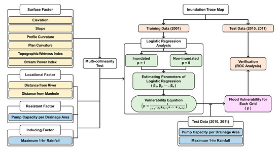
Figure 1.
Flow chart of this study.
2. Study Area and Materials
2.1. Seoul Metropolitan City
Seoul metropolitan city (SMC), the capital city of South Korea, has seen continued population growth with the progress of industrialization and urbanization since the 1960s. As a result, this city is not only a densely populated region with more than 10 million people, which is 20% of the total population of the country, on an area of 605 km2, but also shows a concentration of capital in highly dense office regions such as Gwanghwamun and Gangnam. In this environment, severe flooding occurred in 2010 and 2011, causing great damage to life and property in Seoul. The flood that occurred on 21 September 2010 flooded 17,905 households and injured one person. The flood of 27 July 2011 inundated 14,809 households, causing 19 deaths and 41 injuries [21]. With flood damage occurring every year since then, the city of Seoul has been striving to prevent it by increasing the design frequency of drainage pipes and installing pump stations.
In this study, inundation trace maps generated in 2001 [26] were used to develop a logistic regression model to calculate flood vulnerability for each grid. The inundation trace maps for 2010 and 2011 were used to evaluate the performance of the developed regression model. Figure 2 shows the extent of the study area and the traces of flooding in 2001.
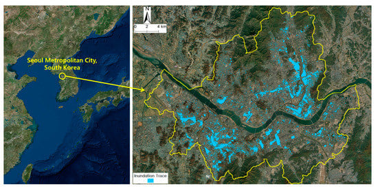
Figure 2.
Inundation traces that occurred in 2001 in Seoul, the study area.
2.2. Hydrological-Topographic Factors
Hydrological-topographic factors were classified into three topographic factors (surface, locational, and resistant) and one hydrological factor (inducing factor). Elevation, slope, profile curvature, plan curvature, topographic wetness index (TWI), and stream power index (SPI) were considered for surface factors, which are the characteristics of runoff moving on the surface by gravity. For locational factors, distance from river and manhole were considered to indicate the range affected by catchment runoff due to natural factors (river) and artificial factors (manhole). As a resistant factor, pump capacity per drainage area was analyzed to consider the effect of drainage pumps installed to protect against urban flooding. The maximum 1-h rainfall was used as an inducing factor, which is an external factor that can directly affect the occurrence of floods.
2.2.1. Surface Factors
The characteristics of surfaces that are vulnerable to flooding are typically lowlands, gentle slopes, and concave terrains, and can be estimated through spatial analysis. In this study, a digital topographic map drawn to a scale of 1:5000 (2018) provided by the NGII [27] was used to calculate the topographic factors of the study area. The digital topographic map was converted into a 30 × 30 m digital elevation model (DEM) through spatial analysis because the contour lines and elevation points were composed in a vector form. Raster calculations were performed with this DEM (elevation) to calculate five surface factors including slope, profile curvature, plan curvature, topographic wetness index, and stream power index (Figure 3).
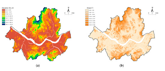
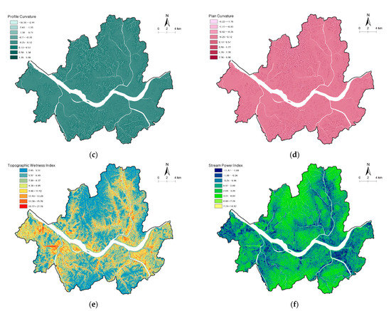
Figure 3.
Topographic factors: (a) Elevation; (b) Slope; (c) Profile curvature; (d) Plan curvature; (e) Topographic wetness index (TWI); (f) Stream power index (SPI).
Elevation is the most representative factor explaining the characteristics of a surface that is prone to flooding; more lowlands means the area is more vulnerable to flooding. Since the flow velocity is slow in areas with gentle slopes, the runoff from rainfall accumulates and causes a flood. Curvature can be calculated as the second derivative of the surface, and can be classified into profile curvature and plan curvature, respectively, depending on whether it is calculated in a direction parallel to or perpendicular to the slope. Profile curvature is the curvature in the downward direction of the slope, and flooding is likely to occur in a concave terrain (positive). Plan curvature is the curvature in the horizontal direction of the slope, and runoff is likely to accumulate in a valley (negative). The topographic wetness index (TWI) was derived from the study of Beven and Kirkby [30] and can be calculated as shown in Equation (1). The TWI means that the gentler the slope () of the target grid and the larger the basin area () of the upstream region, the higher the potential wetness index of the region. The stream power index (SPI), which was proposed by Moore et al. [31], represents the degree of sediment movement and erosion from surface runoff, and is calculated as shown in Equation (2).
2.2.2. Locational Factors
Runoff from rainfall that reaches the ground flows from high to low along the slope by gravity. In natural basins, rainfall runoff gathers to form a river, while in urban areas such runoff is concentrated to manholes through a drainage pipe network. Therefore, areas near rivers or manholes are likely to be vulnerable to flooding when localized torrential downpours exceeding the capacity occur. To calculate the distance from the river and manhole, the location of the river and manholes was calculated for each grid using a digital topographic map (Figure 4a,b).
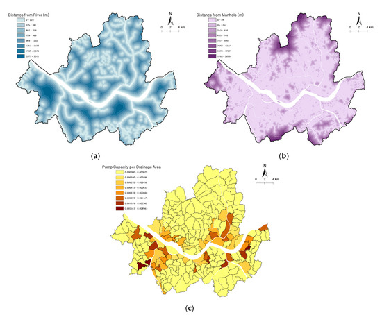
Figure 4.
Locational and resistant factors: (a) Distance from river; (b) Distance from manhole; (c) Pump capacity per drainage area.
2.2.3. Resistant Factor
In urban areas, drainage pumping stations, which are representative facilities to reduce flood damage in lowlands during localized torrential rain, are installed [32]. In this study, statistical data from the Ministry of Environment (ME) [33] were collected to investigate the location and specifications of drainage pumping stations in the study area. On the other hand, since the specific time of the establishment of drainage pumping stations and that of the increase in the capacity could be not confirmed, the year-end statistical data of a year before the flood event, which was applied to the development and verification of this model, were used. It was found that 91 pumping stations were operated in Seoul in 2000, and the total pumping capacity was 118,196 m3/min. In addition, there were 239 drainage sections in Seoul, and each drainage pumping station was designed to fit the area of the drainage section where the facility was located. Therefore, to reflect this, pumping capacity (, m3/min) was divided by the area (, m2) of the drainage section to calculate pumping capacity per drainage area (), as shown in Equation (3) (Figure 4c).
2.2.4. Inducing Factor
Recently, the frequency of localized torrential rains has been increasing due to climate change [34]. In Seoul, which was affected by this, the number of occurrences of more than 30 mm/h of rainfall increased by 2.3 times throughout the year compared to before 1990, and that of more than 50 mm/h of rainfall increased by 5.3 times [35]. In addition, Son et al. [35] analyzed that rainfall of 75.0 mm and 15.5 mm/h was observed at the Seodaemun (412) and Dobong (406) observatories in Seoul at 14:00 on 21 September 2010, respectively, showing an approximately 5-fold difference between the two observatories. As such, in terms of the temporal distribution of rainfall, the occurrence frequency of concentrated torrential rains (30 mm/h or more) increases, and the spatial distribution also shows a large deviation due to localized heavy rains. Therefore, it was confirmed that topographic and hydrological factors should be connected when estimating flood vulnerability in this study.
Inundation damage in Seoul resulted mainly from inland floods, which occurred in urban lowlands or were caused by rainfall that could overwhelm the drainage infrastructure, rather than fluvial floods [21]. In Korea, when designing drainage pipes to protect against flood, the rainfall duration and the return period generally considered are 1 h and 10–30 years, respectively [36]. Therefore, in this study, maximum 1-h rainfall was used as an inducing factor that causes urban flooding.
Korea Meteorological Administration (KMA) [29] provides various types of observation data, such as automated synoptic observing system (ASOS) and automated weather system (AWS), as shown in Table 1. ASOS is installed in the location of the former KMA to perform observation tasks such as observing weather phenomena and data sharing through international cooperation, and AWS is installed in places where observation by a human operator is difficult, such as on mountains or islands, to monitor localized severe weather phenomena in real time [37]. There were a total of 32 rainfall observatories located in and near Seoul, as shown in Table 1, but to secure the reliability of the data required to develop a regression model, it was necessary to select data in consideration of missing observations, and the opening/closure of such observatories. The data from the Gangseo (404) and Gwangjin (413) observatories were excluded because missing data were found at the time of the occurrence of maximum 1-h rainfall observed at a nearby observatory in 2001. Those from Bukaksan (422), Guro (423), Gangbuk (424), and Namhyeon (425) observatories were excluded because they opened after 2001. The selected data were interpolated using the inverse distance weighting (IDW) method to assign the rainfall at the point where the observatories were located to all the relevant grids (Figure 5).

Table 1.
Observatories in Seoul and maximum 1-h. rainfall.
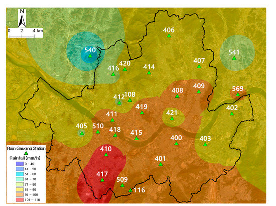
Figure 5.
Rainfall interpolation result (2001).
On the other hand, inundation trace maps provided information on flooded areas, but did not provide information on the date and time of flooding. If information on the time of flooding is not available, such data cannot be linked to rainfall data. Therefore, in this study, the maximum 1-h rainfall occurring in July 2001 was used as an independent variable for logistic regression. After that, to evaluate the performance of the regression equation, flood vulnerability was estimated using the maximum 1-h rainfall in September 2010 and July 2011, and compared with the inundation trace maps.
3. Methodology
3.1. Multi-Collinearity Test
Multi-collinearity problems can cause when there is a correlation between two or more variables in a regression model. This problem can cause the calculations to be false, and the logistic parameters are incorrect and or inexact [38]. As the surface factors used in this study, five independent variables (slope, profile curvature, plan curvature, TWI, and SPI) calculated from elevation were used. Applying variables derived from one raster data to a regression model may cause multi-collinearity problems [17]. Therefore, the determination of multi-collinearity is an important step in detecting flood vulnerability using a logistic regression model. The variance inflation factor (VIF), one of the indicators used to determine multi-collinearity, can be calculated using the coefficient of determination () as in Equation (4).
Lin [39] stated that variables can be judged to have multi-collinearity when VIF is greater than 10. Table 1 shows that there is no multi-collinearity problem as the VIF values for the six independent variables of the surface factors ranged from 1.099 to 2.679 (Table 2). Therefore, it was confirmed that six surface factors can be used as independent variables in logistic regression analysis to calculate flood vulnerability.

Table 2.
Evaluation of vulnerability according to area under the curve (AUC).
3.2. Logistic Regression
Logistic regression is a probability model proposed by Cox [40], which is used for classification and prediction by expressing the relationship between dependent variables and independent variables as a regression equation. It was mainly proposed to classify events in which the dependent variable follows a binomial distribution, such as the relationship between test scores and whether they pass the exam, or patient health status and whether they have a disease.
Odds ratio (OR) was introduced to utilize logistic regression for binary classification. OR represents the ratio of the probability, , that an event will occur, and the probability, , that it will not occur, and it is calculated as follows.
In addition, the problem of binary classification is that a linear regression analysis cannot be performed, because the dependent variable is represented as “0” or “1”, and thus the range is different from the independent variable having a continuous distribution. Accordingly, the dependent variable is adjusted to (−∞, ∞) in the range of [0, 1] through the logit transformation that applies the logarithm to OR. This can be expressed using the following equation.
In this study, for the calculation of the regression coefficient () of Equation (6), the occurrence of flooding events () for all grids in the study area and 10 hydrological-topographic factors () were used. In addition, the maximum likelihood estimator is used to determine regression coefficients including the constant term [41].
Next, a logistic function is used to calculate the flooding probability for target grids using the calculated regression coefficients. The logistic function can be calculated as follows by using the inverse function relation in Equation (6).
The probability of flooding can be obtained by inputting the hydrological-topographic factor for a target grid to Equation (10). This flooding probability corresponds to flood vulnerability in this study. The flood vulnerability estimated through the logistic regression has the range [0, 1], and the closer to 1, the higher the probability of flood occurrence.
3.3. 2 × 2 Confusion Matrix and ROC Analysis
In this study, a receiver operating characteristics (ROC) analysis was conducted using a 2 × 2 confusion matrix to check the extent to which the areas with high flood vulnerability calculated using the logistic regression model were consistent with the inundation trace maps. The 2 × 2 confusion matrix and ROC analysis have been mainly used in the medical field, including the performance evaluation of reagents that discriminate negative from positive patients in the diagnostic test of COVID-19, which has been spreading around the world in recent years. This technique has recently been extended and applied to the fields of machine learning and object recognition to evaluate the classification accuracy of artificial intelligence [42,43]. ROC analysis allows us to determine whether a test method is useful by showing a curve for the degree to which an event is detected for each test method [44,45]. To draw this curve, four components of a 2 × 2 confusion matrix should be used.
As shown in Table 3, the 2 × 2 confusion matrix can be composed of 4 different combinations depending on whether the flood vulnerable area and inundation traces on the map coincide. If the flood vulnerable area and inundation traces coincide, it can be expressed as true positives (TP) or true negatives (TN); otherwise, it is expressed as false positives (FP) or false negatives (FN). For the plot of the ROC curve, the x-axis is calculated as 1-specificity, showing specificity which is the ratio of accurately predicted areas (TN) among the areas where no actual flooding occurred (FP + TN). The y-axis of the graph shows sensitivity, which is the ratio of the areas selected as flood vulnerable areas (TP) among the flooded areas (TP + FN). When expressed as an equation, specificity and sensitivity can be expressed as Equations (11) and (12), respectively, and the range of values is [0, 1] [45].

Table 3.
Overview of 2 × 2 confusion matrix.
In ROC analysis, the performance of a test method can be evaluated by calculating the area under the curve (AUC). It can be evaluated that the closer the AUC is to 1, the better the detection performance is, while the closer the AUC is to 0, the worse the detection performance is. According to Ying et al. [46] and Simundic [47], the AUC can be evaluated as shown in Table 4. In addition, if the ROC curve is distributed below the diagonal with a slope of 1 and the AUC is calculated to be 0.5 or less, it means that the test method is not useful.

Table 4.
Evaluation of vulnerability according to area under the curve (AUC).
4. Results and Discussion
4.1. Logistic Regression Modeling
For the analysis, the city of Seoul was divided using a grid into 648,174 30 m × 30 m squares excluding rivers, and 47,065 of these were found to have inundation traces. Through this process, the grid where flooding had occurred and those where it had not were classified as 1 and 0, respectively, and these values were entered into Y of Equation (5). In addition, the hydrological-topographic factors for each grid were required in the logistic regression equation to estimate the flood vulnerability. This study intends to provide information on the changes in vulnerability according to rainfall, rather than calculating unchanged flood vulnerability for each grid by considering only the topographic factors. Therefore, two logistic regression models were developed and their performance was compared: an equation that used only topographic factors (T) as independent variables, and one that also included hydrological factors (TR). As a result, the logistic regression coefficients and constant terms of the two equations were determined, as shown in Equations (14) and (15), respectively.
With the data for 2001, the flood vulnerability was calculated using the hydrological-topographic factors and the determined regression coefficients, for all grid in the study area (Figure 6). In the figure, a darker color indicates that the area is more vulnerable, while a lighter color indicates that the area is less vulnerable. The flood vulnerability was represented by classifying the probability in the range [0, 1] into five classes using the natural breaks method. The idea of the natural breaks method is to minimize variance among objects within the chosen subsets, and maximize variance between the subsets [48]. The five classes included very high (1.00–0.50), high (0.50–0.34), medium (0.34–0.22), low (0.22–0.13), and very low (0.13–0.02). In addition, as areas with a probability of less than 2% were not evaluated to be vulnerable, a vulnerability level was not assigned to these.
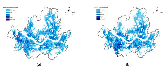
Figure 6.
Results of logistic regression (2001): (a) Topographic data; (b) Topographic and hydrological data.
Flood vulnerability, which was calculated with two logistic regression equations, was divided into vulnerability considering only topographic factors (Figure 6a) and one that also considered maximum 1-h rainfall, a hydrological factor (Figure 6b). From the difference between Figure 6a,b, it can be seen that the vulnerability varies by region according to the spatial distribution of the maximum 1-h rainfall. When considering the hydrological factor, the area with very high-intensity rainfall of 100–110 mm/h (the area marked in red in the southwest in Figure 5) was more susceptible to flooding than when only topographic factors were considered. On the other hand, the area with rainfall of 60–70 mm/h (the area represented in green in the northwest in Figure 5) was found to be less vulnerable.
An ROC analysis was conducted to quantitatively confirm whether the flood vulnerable areas determined by the technique proposed in this study and those where floods occurred in the past coincided. To plot the ROC curve with 10 points, the flood vulnerability of target areas was divided into 10 equal parts using quartiles. If many floods occurred in areas with high vulnerability in the ROC curve (lower side of the x-axis), the sensitivity would increase, and in particular would increase sharply at the beginning of the curve. Consequentially, as the AUC increases, it can be evaluated that the technique of this study detects flooded areas well. The ROC curve is shown in Figure 7.
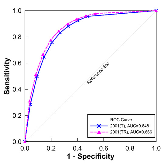
Figure 7.
ROC curves of flood vulnerability and inundation traces.
Through ROC analysis, it was found that the AUC of flood vulnerability considering only topographic factors and that including rainfall were 0.848 and 0.866, respectively, and both were evaluated as “very good” as shown in Table 4. Further, the precision was calculated to confirm the rate at which flood occurrence was detected for the flood vulnerability, which was classified into five classes. This can be obtained by using the number of samples classified as positive in a 2 × 2 confusion matrix as shown in Equation (16), and the range is [0, 1] (perfect value is 1) [49,50]. The precision for each class was calculated as shown in Figure 8 and, in both cases, it was found that floods were detected at a rate of more than 50% in the very high class, and more than 40% in the high class.
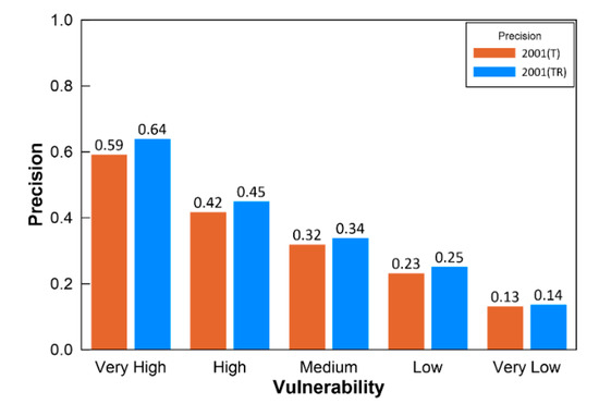
Figure 8.
Proportion of flood occurrence in vulnerable areas.
Based on the results of this analysis, it is considered that the logistic regression model detects flood occurrence well in the study area. Although the inputting of the hydrological factor did not make a distinct difference, it can be assumed that the vulnerability will change and the detection rate will improve if new rainfall data are input, even without topographic changes. To confirm this, the performance of the logistic regression equation was evaluated using the maximum 1-h rainfall and inundation trace maps in 2010 and 2011.
4.2. Mapping Vulnerable Areas in Other Flood Events
To evaluate the performance of the logistic regression model developed in this study, inundation trace maps and the maximum 1-h rainfall data were collected for floods that occurred in September 2010 and July 2011. Of the rainfall observatories, the Bukaksan (422) and Namhyeon (425) observatories were excluded because they had not yet opened in 2010, and the Bukhansan (420) observatories, which were closed in 2011, were also excluded. The rainfall of the observatories was interpolated using the IDW method as shown in Figure 9. In 2010, very high-intensity rainfall of around 100 mm/h occurred in the west of the study area, while relatively low-intensity rainfall of around 60 mm/h was recorded in the north. Overall, in 2011, it rained less than in 2010, except in the south with 100 mm/h of rainfall.
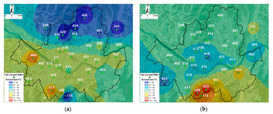
Figure 9.
Rainfall interpolation results by year: (a) September 2010; (b) July 2011.
In addition, the year-end statistical data for 2009 and 2010 [51,52] were used to consider drainage pumping stations that were newly built or increased in capacity after flooding in 2001. In 2009 and 2010, the number of pumping stations was increased from 91 in 2000 to 111, and the capacity also was increased to 155,313 m3/min (2009) and 161,279 m3/min (2010). The changed pump capacity per drainage area is shown in Figure 10.
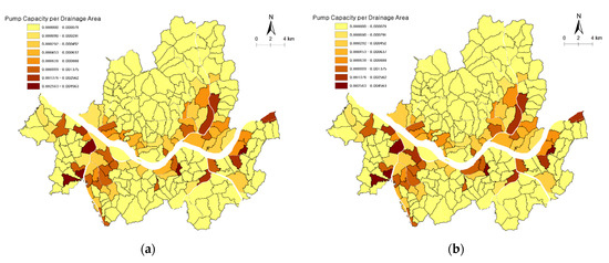
Figure 10.
Density of drainage pump capacity by year: (a) September 2010; (b) July 2011.
In the logistic regression model developed above with data for 2001, the same values as those in 2001 were used for surface and locational factors, and values for 2010 and 2011 were entered for resistant and inducing factors, respectively. The flood vulnerability that was recalculated by inputting pumping capacity and rainfall to this model is shown in Figure 11. Interestingly, as low rainfall was input compared to that used in the development of the model, the vulnerability in 2010 and 2011 was decreased significantly compared to in 2001. In addition, in 2010, the high-intensity rainfall in the west increased the vulnerability, and the low-intensity rainfall in the north decreased the vulnerability. In 2011, most areas were calculated to have low vulnerability, except for the increase in vulnerability in some areas due to high-intensity rainfall in the south.
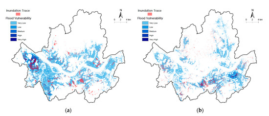
Figure 11.
Results of the selection for flood vulnerable areas: (a) September 2010; (b) July 2011.
An ROC analysis was conducted to quantitatively analyze the extent to which calculated flood vulnerability in 2010 and 2011 actually detects floods. The ROC curves for 2010 and 2011 are shown in Figure 12. In both cases, it was found that the measure of flood vulnerability (AUC = 0.861, 0.815) that considered the hydrological factors together detected flood occurrence better than that (AUC = 0.841, 0.766), which considered only the topographic factors. The detection rate was calculated as shown in Figure 13. In 2010, among vulnerable areas considering rainfall, flooding occurred at a rate of 66% (T, 57%) in the very high class; 54% (T, 31%) in the high; 47% (T, 18%) in the medium; 33% (T, 12%) in the low; and 11% (T, 7%) in the very low. In 2011, floods occurred at a rate of 36% (T, 17%) in the very high class; 41% (T, 12%) in the high; 31% (T, 9%) in the medium; 28% (T, 6%) in the low; and 9% (T, 4%) in very low. Through ROC analysis and precision, it was found that the model for calculating flood vulnerability that only considers topographic factors has a disadvantage of overestimating vulnerable areas, but that the detection rate could be improved by up to over four times (in the low class in 2011) when the rainfall was also considered.
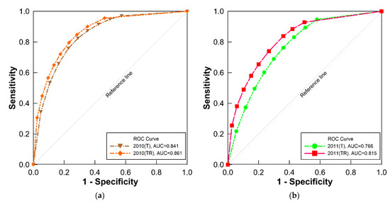
Figure 12.
ROC curves of flood vulnerability and inundation traces for performance evaluation: (a) September 2010; (b) July 2011.
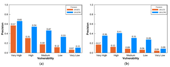
Figure 13.
Proportion of flood occurrence in vulnerable areas for performance evaluation: (a) September 2010; (b) July 2011.
4.3. Discussion
This study proposed a technique for calculating the flood vulnerability that changes according to the rainfall situation using hydrological-topographic factors. Lee et al. [5] suggested that studies using globally available data, such as SRTM and ASTER, are needed so that they can be used even in areas where data are insufficient in flood vulnerability analysis. In addition, they said that it is necessary to develop a technique that can evaluate flood vulnerability in a simple but scientific way that can be applied to areas where there are no data on hydrological observations or poor quality. Against this background, in this study, topographic data that can be used anywhere was used as an independent variable of the logistic regression model, and data on soil or land use, which may not be available depending on the region, were not added. However, reviewing previous studies, 89% of the floods that occurred in Seoul in 2011 occurred in areas with an impermeability rate of 70% or higher [21]. Further, it was analyzed that 52.1% of the study area consisted of roads, residential, and commercial areas, and 89.4% of floods occurred in these areas. It would be good if soil impermeability or land use is added as an independent variable through future research.
In this study, flood vulnerability was calculated using hydrological-topographic factors and compared with historical inundation trace data. As a result, there were some cases where flooding occurred in areas with a calculated vulnerability lower than 0.5, and other cases where flooding did not occur even in areas above 0.5. However, it remains uncertain whether areas with relatively low vulnerability are safer. It is true that areas with high vulnerability require intensive management due to their high probability of flooding, but even areas with low vulnerability should be managed with constant attention to reduce flood damage. Since floods occur for very complicated causes, it may be difficult to detect them using only the factors used in this study. Kim et al. [53] proposed an optimal input data selection method by combining total rainfall, rainfall of various durations, kurtosis, and skewness to predict urban flooding using a deep neural network. If the characteristics of rainfall, such as various durations, kurtosis, and skewness, are considered as an inducing factor, the detection accuracy for flood vulnerable areas can be improved.
The flood vulnerability, calculated using hydrological-topographic factors, did not take into account the density and importance of the population and capital in the study area. If a flood occurs in a densely populated area, it is difficult for many people to evacuate all at once, so even if the area has a low vulnerability, it is necessary to pay close attention to the area. Similarly, in areas where major social overhead capital (SOC) facilities are located, such as power plants or water supply/wastewater treatment facilities, great damage can be caused to surrounding areas when floods occur. Rehman et al. [54] reviewed scholarly articles related to flood vulnerability from 1990 to 2018, noting that flood vulnerability is being analyzed in social, environmental, and economic contexts, and presented a list of indicators that can be used for future research. In this regard, it is necessary to distinguish the vulnerability of regions with high socio-economic vulnerability from the criteria for calculating flood vulnerability ratings for other regions.
Another point to be improved in the methodology of this study is that the vulnerability of the entire study area was calculated using one logistic regression equation. Accordingly, there is a limitation in that areas with the same hydrological-topographic factors are likely to be determined as vulnerable areas even though flood damage did not occur there. These areas may not actually be flooded due to flood protection facilities such as a retarding basin, or drainage pipe networks that have already been expanded to handle the greater amount of rainfall through local government management. Based on this, a good direction for a future study would be to develop a logistic regression equation for each drainage section rather than only one equation for the entire study area. It is considered that the disaster prevention performance of the drainage section can be reflected indirectly through such equations without using a physical model.
5. Conclusions
In this study, we proposed a technique to detect flood vulnerable areas by simultaneously considering topographic and hydrological factors to reduce damage caused by flooding. To estimate the vulnerability to flooding of the study area, a logistic regression model was developed using historical inundation trace data, and hydrological-topographic factors based on the grid system. The conclusions obtained through this study are as follows.
- (1)
- A logistic regression model was established by dividing into a model that only considered topographic factors (T) and one that included hydrological factors (TR), and the results were compared. When comparing the two models, it was found that the estimated result was different due to the influence of rainfall. In addition, according to the results of ROC analysis and precision calculation, it was found that the method of estimating the flood vulnerability that included the hydrological factor was relatively better for detecting the flood occurrence pattern.
- (2)
- Flood events in 2010 and 2011 were applied to evaluate the performance of the developed logistic regression model. Through ROC analysis with inundation trace maps, it was found that the AUC improved from 0.841 (T) to 0.861 (TR) in 2010, and from 0.766 (T) to 0.815 (TR) in 2011, indicating that the model including hydrological factors was better for detecting flooding patterns. In addition, according to the actual flood occurrence rates calculated in the vulnerable areas determined in consideration of the rainfall, the detection rate was significantly improved compared to the approach that considered only topographical factors, which overestimated vulnerable areas.
- (3)
- There were some cases in which flooding occurred in areas with low vulnerability, while in other cases, high vulnerability areas saw no floods occur. The cause of a flood is very complicated because the factors influence the events in a complex manner through interaction. Therefore, constant attention and management is required even for areas with low vulnerability. In particular, areas with many residents or important SOC facilities should be managed separately.
- (4)
- The technique for determining flood vulnerable areas proposed in this study enables an analysis to be performed quickly and conveniently because the topographic factors are fixed in the logistic regression equation and only new rainfall is inputted to it. If real-time rainfall forecasting is available, it will allow us to quickly and easily predict areas that are likely to be flooded. In addition, through further research, if a regression model for each drainage section is developed by subdividing the characteristics of flood damage factors, it is expected that the detection rates will improve and more reliable flood information will be provided.
Author Contributions
Conceptualization, J.-Y.L. and J.-S.K.; methodology, J.-Y.L. and J.-S.K.; software and validation, J.-Y.L.; writing—original draft preparation, J.-Y.L.; writing—review and editing, J.-S.K. All authors have read and agreed to the published version of the manuscript.
Funding
This study was supported by a Grant (127568) from the Water Management Research Program funded by Ministry of Environment of Korean government.
Institutional Review Board Statement
Not applicable.
Informed Consent Statement
Not applicable.
Acknowledgments
This study was supported by a Grant (127568) from the Water Management Research Program funded by Ministry of Environment of Korean government.
Conflicts of Interest
The authors declare no conflict of interest.
References
- Koh, T.G.; Lee, W.Y. A Study on Urban Planning Technique for Flood Reduction in the Lowlands. Seoul Stud. 2012, 13, 287–300. [Google Scholar]
- Balica, S.F.; Popescu, I.; Beevers, L.; Wright, N.G. Parametric and Physically Based Modelling Techniques for Flood Risk and Vulnerability Assessment: A Comparison. Environ. Modeling Softw. 2013, 41, 84–92. [Google Scholar] [CrossRef]
- Dehotin, J.; Breil, P.; Braud, I.; Lavenne, A.D.; Lagouy, M.; Sarrazin, B. Detecting Surface Runoff Location in a Small Catchment using Distributed and Simple Observation Method. J. Hydrol. 2015, 525, 113–129. [Google Scholar] [CrossRef]
- Lagadec, L.R.; Patrice, P.; Braud, I.; Charzelle, B.; Moulin, L.; Dehotin, J.; Breil, P. Description and Evaluation of a Surface Runoff Susceptibility Mapping Method. J. Hydrol. 2016, 541, 405–509. [Google Scholar] [CrossRef]
- Lee, K.S.; Lee, D.E.; Jung, S.H.; Lee, G.H. Analysis of Large-scale Flood Inundation Area using Optimal Topographic Factors. J. Korean Water Resour. Assoc. 2018, 51, 481–490. [Google Scholar]
- Lee, J.Y.; Kim, J.S. ROC Analysis of Topographic Factors in Flood Vulnerable Area Considering Surface Runoff Characteristics. Eco. Resilient Infra. 2020, 7, 327–335. [Google Scholar]
- Tehrany, M.S.; Lee, M.J.; Pradhan, B.; Jebur, M.N.; Lee, S.R. Flood Susceptibility Mapping using Integrated Bivariate and Multivariate Statistical Models. Environ. Earth Sci. 2014, 72, 4001–4015. [Google Scholar] [CrossRef]
- Lee, S.M.; Lee, M.J. Susceptibility Mapping of Umyeonsan using Logistic Regression Model and Post-validation through Field Investigation. Korean J. Remote Sens. 2017, 33, 1047–1060. [Google Scholar]
- Jung, M.K.; Kim, J.G.; Uranchimeg, S.; Kwon, H.H. The Probabilistic Estimation of Inundation Region using a Multiple Logistic Regression. J. Korea Water Resour. Assoc. 2020, 53, 121–129. [Google Scholar]
- Wang, Z.; Lai, C.; Chen, X.; Yang, B.; Zhao, S.; Bai, X. Flood Hazard Risk Assessment Model Based on Random Forest. J. Hydrol. 2015, 527, 1130–1141. [Google Scholar] [CrossRef]
- Rizeei, H.M.; Pradhan, B.; Saharkhiz, M.A. An Integrated Fluvial and Flash Pluvial Model using 2D High-resolution Sub-grid and Particle Swarm Optimization-based Random Forest Approaches in GIS. Complex Int. Syst. 2019, 5, 283–302. [Google Scholar] [CrossRef]
- Kalantari, Z.; Nickman, A.; Lyon, S.W.; Olofsson, B.; Folkeson, L. A Method for Mapping Flood Hazard along Roads. J. Envron. Manag. 2014, 133, 69–77. [Google Scholar] [CrossRef] [PubMed]
- Khatun, S.; Pal, S. Categorization of Morphometric Surface through Morphometric Diversity Analysis in Kushkarani River Basin in Eastern India. Asian J. Phys. Chem. Sci. 2017, 2, 1–19. [Google Scholar] [CrossRef]
- Pradhan, B.; Lee, S.R. Delineation of Landslide Hazard Areas on Penang Island, Malaysia, by using Frequency Ratio, Logistic Regression, and Artificial Neural Network Models. Environ. Earth Sci. 2010, 60, 1037–1054. [Google Scholar] [CrossRef]
- Lee, S.M.; Kim, J.C.; Jung, H.S.; Lee, M.J.; Lee, S.R. Spatial Prediction of Flood Susceptibility using Random-forest and Boosted-tree Models in Seoul Metropolitan City, Korea. Geom. Nat. Hazard Risk 2017, 8, 1185–1203. [Google Scholar] [CrossRef]
- Li, X.; Yan, D.; Wang, K.; Weng, B.; Qin, T.; Liu, S. Flood Risk Assessment of Global Watersheds Based on Multiple Machine Learning Models. Water 2019, 11, 1654. [Google Scholar] [CrossRef]
- Nandi, A.; Mandal, A.; Wilson, M.; Smith, D. Flood Hazard Mapping in Jamaica using Principal Component Analysis and Logistic Regression, Environ. Earth Sci. 2016, 75, 465. [Google Scholar] [CrossRef]
- Melly, B.L.; Schael, D.M.; Nick, R.M.; Gama, P.T. Mapping Ephemeral Wetlands: Manual Digitisation and Logistic Regression Modelling in Nelson Mandela Bay Municipality, South Africa. Wetl. Ecol. Manag. 2017, 25, 313–330. [Google Scholar] [CrossRef]
- Sun, X.; Chen, J.; Bao, Y.; Han, X.; Zhan, J.; Peng, W. Landslide Susceptibility Mapping using Logistic Regression Analysis along the Jinsha River and Its Tributaries Close to Derong and Deqin County, Southwestern China. Int. J. Geo-Inf. 2018, 7, 438. [Google Scholar] [CrossRef]
- Korea Institute of Construction Technology (KICT). Investigation Report on Heavy Rainfall in the Metropolitan Region in July 2011; KICT: Goyang, Korea, 2011. [Google Scholar]
- Shin, S.Y.; Park, C.Y. Analyzing Relationships between Land Use Characteristics and Flood Damage Area: The Case of Seoul. Korea Spat. Plan. Rev. 2014, 81, 3–20. [Google Scholar]
- Zhao, G.; Xu, Z.; Pang, B.; Tu, T.; Xu, L.; Du, L. An Enhanced Inundation Method for Urban Flood Hazard Mapping at the Large Catchment Scale. J. Hydrol. 2019, 571, 873–882. [Google Scholar] [CrossRef]
- Kim, B.H.; Sanders, B.F.; Schubert, J.E.; Famiglietti, J.S. Mesh Type Tradeoffs in 2D Hydrodynamic Modeling of Flood with a Godunov-based Flood Solver. Adv. Water Resour. 2014, 68, 42–61. [Google Scholar] [CrossRef]
- Liang, Q.; Du, G.; Hall, J.W.; Borthwick, A.G.L. Flood Inundation Modeling with an Adaptive Quadtree Grid Shallow Water Equation Solver. J. Hydraul. Eng. 2008, 134, 1603–1610. [Google Scholar] [CrossRef]
- Mosavi, A.; Ozturk, P.; Chau, K. Flood Prediction using Machine Learning Models: Literature Review. Water 2018, 10, 1536. [Google Scholar] [CrossRef]
- Seoul Open Data Plaza. Available online: https://data.seoul.go.kr (accessed on 14 October 2020).
- National Geographic Information Institute (NGII). Available online: http://map.ngii.go.kr (accessed on 2 January 2019).
- National Spatial Data Infrastructure Portal. Available online: http://data.nsdi.go.kr (accessed on 14 October 2020).
- Weather Data Open Portal. Available online: https://data.kma.go.kr (accessed on 1 February 2021).
- Beven, K.J.; Kirkby, M.J. A Physically Based Variable Contributing Area Model of Basin Hydrology. Hydrol. Sci. J. 1979, 24, 43–69. [Google Scholar] [CrossRef]
- Moore, I.D.; Grason, R.B.; Ladson, A.R. Digital Terrain Modelling: A Review of Hydrological, Geomorphological, and Biological Applications. Hydrol. Proc. 1991, 5, 3–30. [Google Scholar] [CrossRef]
- Song, Y.H.; Park, M.J.; Lee, J.H. Analysis of Urban Inundation Reduction Effect by Early Operation of Drainage Pumping Station. J. Korean Soc. Hazard Mitig. 2014, 14, 267–276. [Google Scholar] [CrossRef]
- Ministry of Environment (ME). Statistics of Sewerage 2000; ME: Seoul, Korea, 2000.
- Jeong, I.J.; Kim, S.K.; Choi, J.H.; Jung, S.G. A Study on Element Derived for Disaster Recovery Support Priorities. J. Korean Soc. Hazard Mitig. 2016, 16, 67–71. [Google Scholar] [CrossRef]
- Son, A.L.; Han, K.Y.; Bae, S.H. Temporal and Spatial Characteristics Analysis of Rainfall in Seoul. J. Korean Soc. Hazard Mitig. 2013, 13, 83–95. [Google Scholar] [CrossRef][Green Version]
- Ministry of Environment (ME). A Study on the Adequacy of Probability Years when Calculating Design Rainfall for Public Sewer Facilities; ME: Sejong, Korea, 2018.
- Hyun, J.H.; Park, H.S.; Chung, G.H. Effects of the Difference between ASOS and AWS Data on Runoff Characteristics. J. Korean Soc. Hazard Mitig. 2019, 19, 443–449. [Google Scholar] [CrossRef]
- Al-Juaidi, A.E.M.; Nassar, A.M.; Al-Juaidi, O.E.M. Evaluation of Flood Susceptibility Mapping using Logistic Regression and GIS Conditioning Factors. Arab. J. Geosci. 2018, 11, 765. [Google Scholar] [CrossRef]
- Lin, F.J. Solving Multicollinearity in the Process of Fitting Regression Model using the Nested Estimate Procedure. Qual. Quant. 2008, 42, 417–426. [Google Scholar] [CrossRef]
- Cox, D.R. The Regression Analysis of Binary Sequences. J. R. Stat. Soc. 1958, 20, 215–242. [Google Scholar] [CrossRef]
- Lopez, A.V.; Morales, C. Flash Flood Forecasting in Sao Paulo using a Binary Logistic Regression Model. Atm. 2020, 11, 473. [Google Scholar]
- Bae, H.B.; Kwon, O.S. Untact Face Recognition System Based on Super-resolution in Low-resolution Images. J. Korea Multimed. Soc. 2020, 23, 412–420. [Google Scholar]
- Lee, S.M.; Park, K.D.; Kim, I.K. Comparison of Machine Learning Algorithms for Chl-a Prediction in the Middle of Nakdong River (Focusing on Water Quality and Quantity Factors). J. Korean Soc. Water Wastewater 2020, 34, 277–288. [Google Scholar] [CrossRef]
- DeLong, E.R.; DeLong, D.M.; Clarke-Pearson, D.L. Comparing the Areas under Two or More Correlated Receiver Operating Characteristic. Biometrics 1988, 44, 837–845. [Google Scholar] [CrossRef] [PubMed]
- Metz, C.E. Basic Principles of ROC Analysis. Semin. Nucl. Med. 1978, 8, 283–298. [Google Scholar] [CrossRef]
- Ying, G.S.; Maguire, M.; Quinn, G.; Kulp, M.T.; Cyert, L. Vision in Preschoolers Study Group. ROC Analysis of the Accuracy of Noncycloplegic Retinoscopy, Retinomax Autorefractor, and SureSight Vision Screener for Preschool Vision Screening. Invest. Ophthal. Vis. Sci. 2011, 52, 9658–9664. [Google Scholar] [CrossRef]
- Simundic, A.M. Diagnostic Accuracy-part1, Basic Concepts: Sensitivity and Specificity, ROC Analysis, STARD Statement. Point Care J. Near-Patient Testing Tech. 2012, 11, 6–8. [Google Scholar] [CrossRef]
- Jenks, G. The Data Model Concept in Statistical Mapping. Int. Yearb. Cartogr. 1967, 7, 186–190. [Google Scholar]
- Razali, N.; Ismail, S.; Mustapha, A. Machine Learning Approach for Flood Risks Prediction. IAES Int. J. Art. Int. 2020, 9, 73–80. [Google Scholar] [CrossRef]
- Chapi, K.; Singh, V.P.; Shirzadi, A.; Shahabi, H.; Bui, D.T.; Pham, B.T.; Khosravi, K. A Novel Hybrid Artificial Intelligence Approach for Flood Susceptibility Assessment. Environ. Modeling Softw. 2017, 95, 229–245. [Google Scholar] [CrossRef]
- Ministry of Environment (ME). Statistics of Sewerage 2009; ME: Seoul, Korea, 2009.
- Ministry of Environment (ME). Statistics of Sewerage 2010; ME: Seoul, Korea, 2010.
- Kim, H.I.; Lee, J.Y.; Han, K.Y.; Cho, J.W. Applying Observed Rainfall and Deep Neural Network for Urban Flood Analysis. J. Korean Soc. Hazard Mitig. 2020, 20, 339–350. [Google Scholar] [CrossRef][Green Version]
- Rehnam, S.; Sahana, M.; Hong, H.; Sajjad, H.; Ahmed, B.B. A Systematic Review on Approaches and Methods used for Flood Vulnerability Assessment: Framework for Future Research. Nat. Hazard 2019, 97, 975–998. [Google Scholar]
Publisher’s Note: MDPI stays neutral with regard to jurisdictional claims in published maps and institutional affiliations. |
© 2021 by the authors. Licensee MDPI, Basel, Switzerland. This article is an open access article distributed under the terms and conditions of the Creative Commons Attribution (CC BY) license (https://creativecommons.org/licenses/by/4.0/).