
Probabilistic Design of Retaining Wall Using Machine Learning Methods


Abstract
1. Introduction
2. Methods
2.1. Emotional Neural Network
2.2. Symbiotic Organisms Search-Least Square Support Vector Machine
2.2.1. LSSVM
2.2.2. Symbiotic Organisms Search (SOS)
- Generation of the initial population
- Do
- Mutualism
- Commensalism
- Parasitism
- Best solution update
- Until the criteria of stopping are satisfied.
- Data are collected for training the model.
- The LSSVM model is used to analyze the ambiguous nature of input and output. In addition, and are tuned.
- SOS algorithm:This algorithm searches for several combinations of and parameters and makes the best set of these two parameters. In addition, SOS employs mutualism, commensalism, and parasitism phases to improve the fitness value of the solutions reached slowly.
- Evaluation of fitness:For evaluation of the system, a fitness function is developed that measures the accuracy of the learning system. The best combination of and represents the accurate and best fitness value. The dataset is not split randomly, and it is are divided into learning and validation subsets. In addition, to avoid the bias of sampling, 10-fold cross-validation is done. The mean square error (MSE) is utilized by the fitness function for aptness and better representation.
- Criteria of termination:The termination criterion used in this technique is the iteration number inculcated in the SOS algorithm.
- Optimal and parameters:Loop stops and optimal and parameters are reached.
- The optimal set of and parameters are further used for developing the model for testing the data.
- Data testing:The dataset split for testing is tested, and the prediction is used for assessing the performance and accuracy of the model.
2.3. Multivariate Adaptive Regression Splines
2.4. Cross-Validation
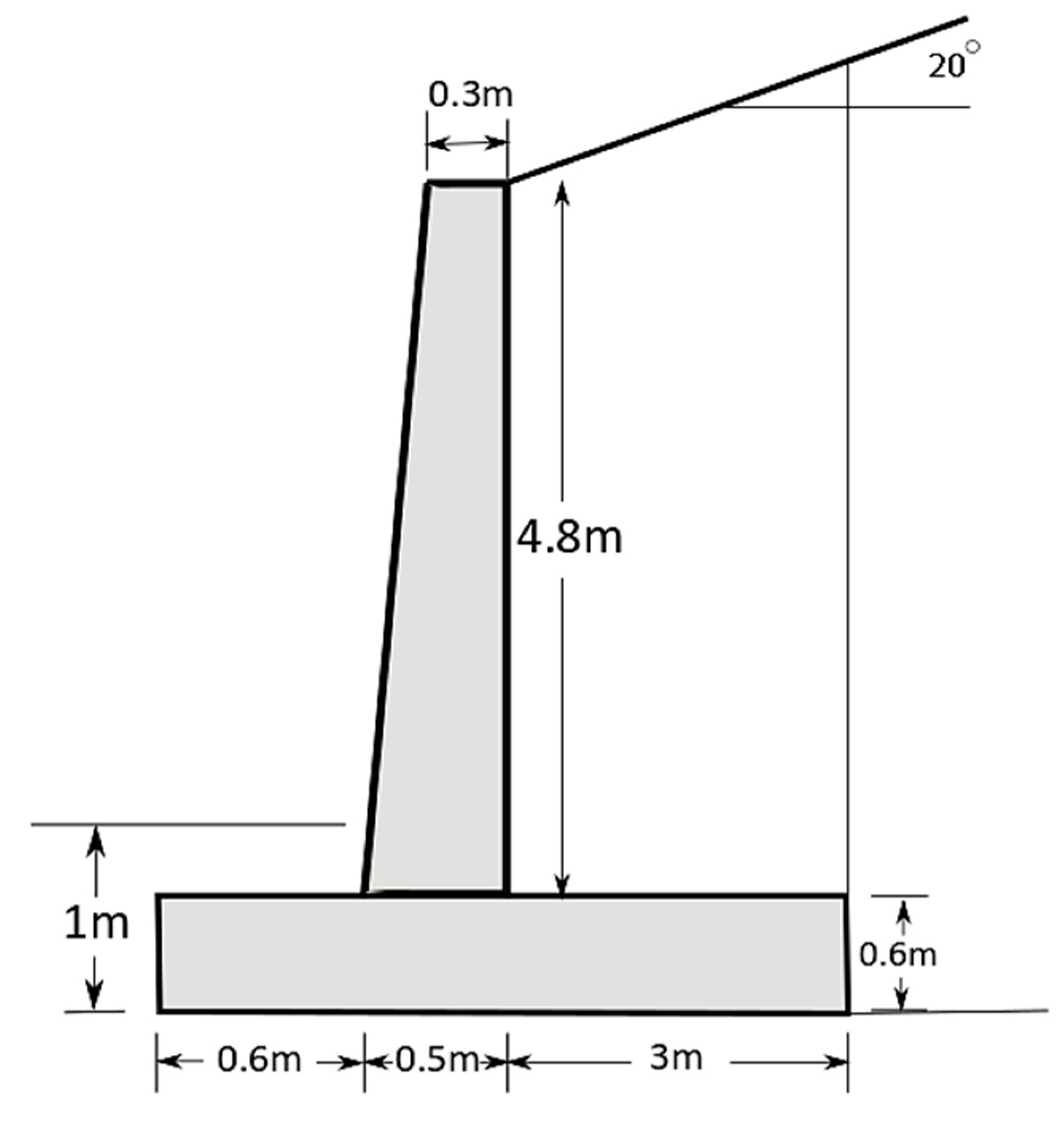
3. Case Example
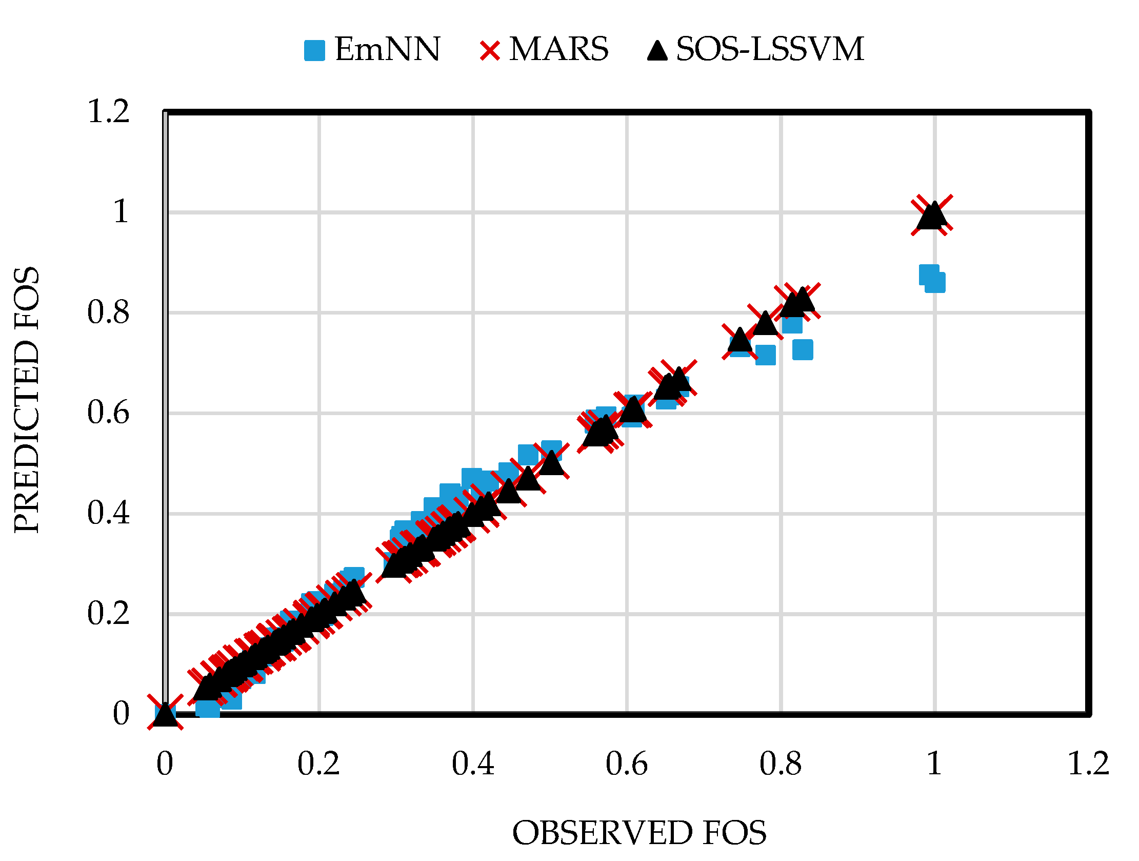
4. Result and Performance Assessment of Models
4.1. Errors and Other Parameters
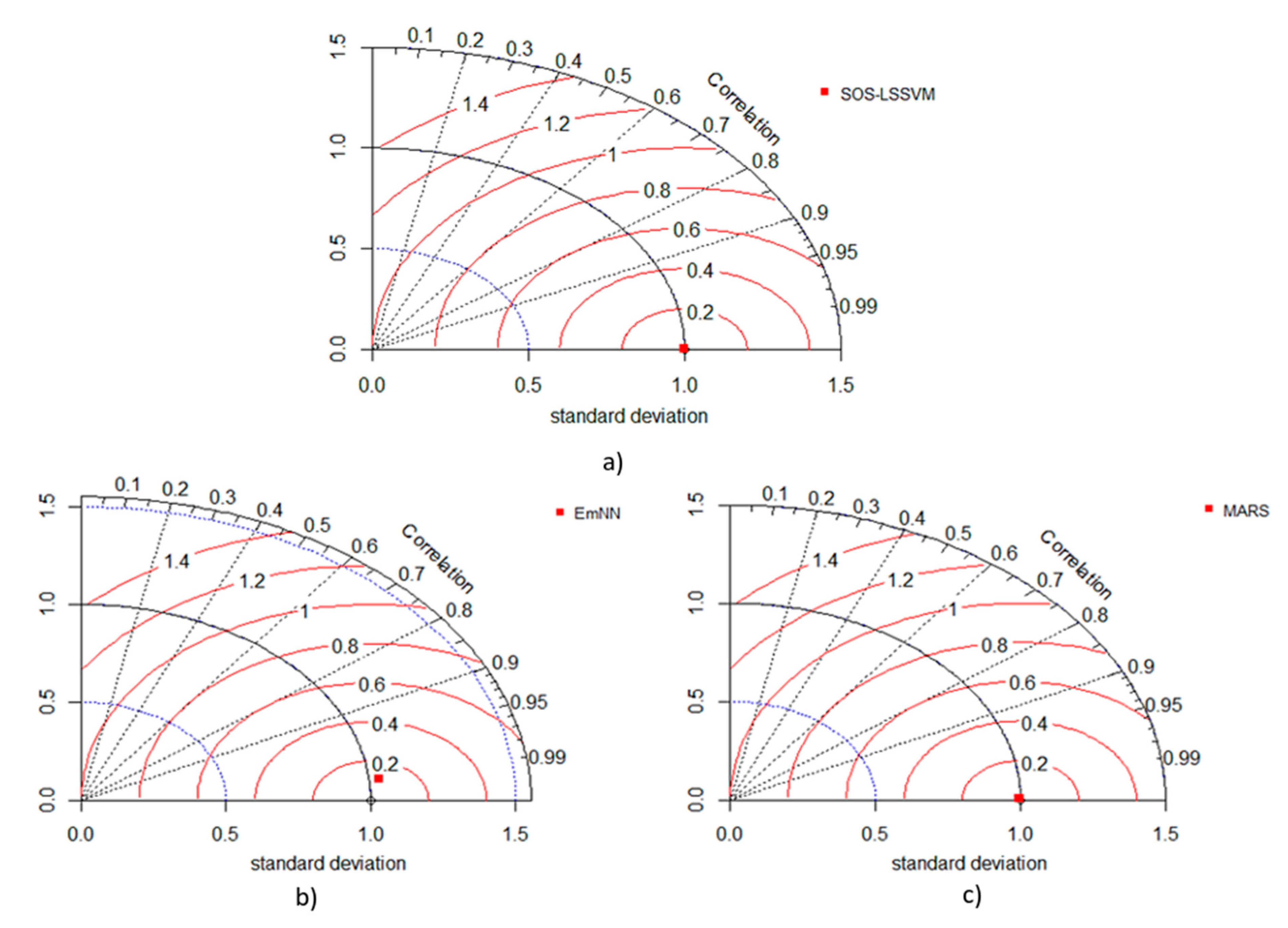
4.2. Taylor Diagram
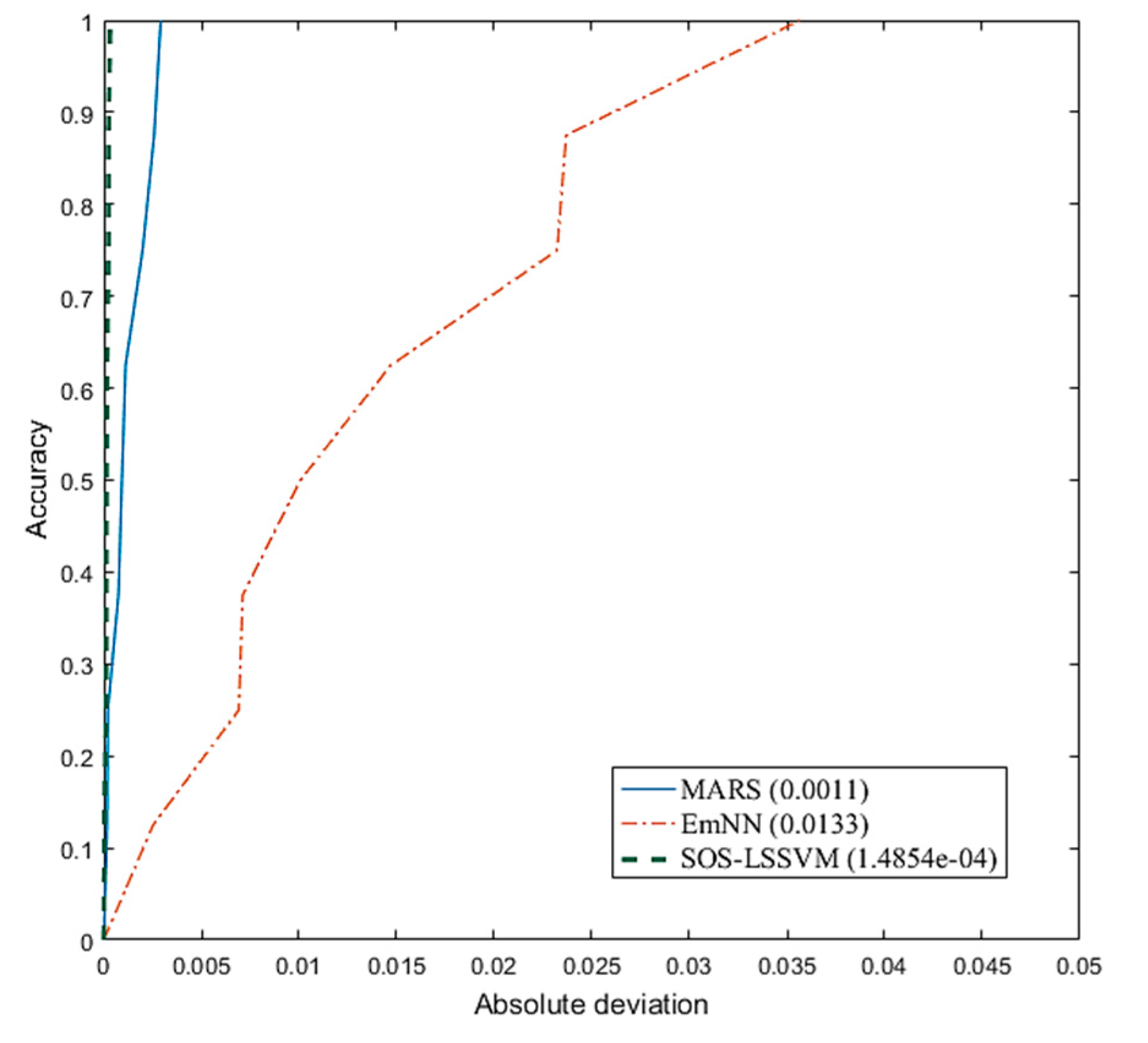
4.3. AOC–REC Curve
4.4. R Curve
5. Conclusions
Author Contributions
Funding
Institutional Review Board Statement
Informed Consent Statement
Data Availability Statement
Conflicts of Interest
References
- Baecher, G.B.; Christian, J.T. Reliability and Statistics in Geotechnical Engineering; Wiley: New York, NY, USA, 2003. [Google Scholar]
- Basha, B.M.; SivakumarBabu, G.L. Optimum design of cantilever sheet pile walls in sandy soils using inverse reliability approach. Comput. Geotech. 2008, 35, 134–143. [Google Scholar]
- Chen, H.; Asteris, P.; Armaghani, D.J. Assessing Dynamic Conditions of the Retaining Wall: Developing Two Hybrid Intelligent Models. Appl. Sci. 2019, 9, 1042. [Google Scholar] [CrossRef]
- Goh, A.T.; Phoon, K.K.; Kulhawy, F.H. Reliability Analysis of Partial Safety Factor Design Method for Cantilever Retaining Walls in Granular Soils. J. Geotech. Geoenviron. Eng. 2009, 135, 616–622. [Google Scholar] [CrossRef]
- Goh, A.T.C.; Kulhawy, F.H. Reliability assessment of serviceability performance of braced retaining walls using a neural network approach. Int. J. Numer. Anal. Meth. Geomech. 2005, 29, 627–642. [Google Scholar] [CrossRef]
- He, L.; Yong, L.; Wang, L.; Broggi, M.; Beer, M. Estimation of Failure Probability in Braced Excavation using Bayesian Networks with Integrated Model Updating. Undergr. Space 2020, 5, 315–323. [Google Scholar] [CrossRef]
- Deng, J.; Gu, D.; Li, X.; Yue, Z. Structural reliability analysis for implicit performance functions using artificial neural network. Struct. Saf. 2005, 27, 25–48. [Google Scholar] [CrossRef]
- Gomes, H.M.; Awruch, A.M. Comparison of response surface and neural network with other methods for structural reliability analysis. Struct. Saf. 2004, 26, 49–67. [Google Scholar] [CrossRef]
- Wu, C.Z.; Goh, T.C.A.; Zhang, W.G. Study on Optimization of Mars Model for Prediction of Pile Drivability Based on Cross—Validation; ISSMGE: Singapore, 2019. [Google Scholar]
- Biswas, R.; Samui, P.; Rai, B. Determination of compressive strength using relevance vector machine and emotional neural network. Asian J. Civ. Eng. 2019, 20, 1109–1118. [Google Scholar] [CrossRef]
- Samui, P. Multivariate adaptive regression spline (Mars) for prediction of elastic modulus of jointed rock mass. Geotech. Geol. Eng. 2012, 31, 249–253. [Google Scholar] [CrossRef]
- Zhang, W.; Goh, A.T. Multivariate adaptive regression splines and neural network models for prediction of pile drivability. Geosci. Front. 2016, 7, 45–52. [Google Scholar] [CrossRef]
- Attoh-Okine, N.O.; Cooger, K.; Mensah, S. Multivariate adaptive regression (MARS) and hinged hyperplanes (HHP) for doweled pavement performance modeling. Constr. Build. Mater. 2009, 23, 3020–3023. [Google Scholar] [CrossRef]
- Cheng, M.Y.; Cao, M.T. Accurately predicting building energy performance using evolutionary multivariate adaptive regression splines. Appl. Soft Comput. 2014, 22, 178–188. [Google Scholar] [CrossRef]
- Cheng, M.Y.; Prayogo, D.; Tran, D.H. Optimizing multiple-resources leveling in multiple projects using discrete symbiotic organisms search. J. Comput. Civ. Eng. 2016, 30, 04015036. [Google Scholar] [CrossRef]
- Prayogo, D.; Susanto, Y.T.T. Optimizing the prediction accuracy of friction capacity of driven piles in cohesive soil using a novel self-tuning least squares support vector machine. Adv. Civ. Eng. 2018, 2018, 1–9. [Google Scholar] [CrossRef]
- Babu, G.; Srivastava, A. Reliability analysis of buried flexible pipe-soil system. J. Pipeline Syst. Eng. Pract. 2010, 1, 33–41. [Google Scholar] [CrossRef]
- Wu, T.H.; Kraft, L.M. Safety analysis of slopes. J. Soil Mech. Found. Div. 1970, 96, 609–630. [Google Scholar] [CrossRef]
- Mahmoudi, E.; Khaledi, K.; Miro, S.; Koenig, D.; Schanz, T. Probabilistic Analysis of a Rock Salt Cavern with Application. Rock Mech. Rock Eng. 2017, 50, 139–157. [Google Scholar] [CrossRef]
- Tang, W.H.; Yucemen, M.S.; Ang, A.H.S. Probability-based short term design of slopes. Can. Geotech. J. 1976, 13, 201–215. [Google Scholar] [CrossRef]
- Cornell, C. First-order uncertainty analysis of soils deformation and stability. In Proceedings of the 1st International Conference on Application of Probability and Statistics in Soil and Structural Engineering, Hong Kong, China, 13–16 September 1971. [Google Scholar]
- Levine, D.S. Neural network modeling of emotion. Phys. Life Rev. 2007, 4, 37–63. [Google Scholar] [CrossRef]
- Fragopanagos, N.; Taylor, J.G. Modelling the interaction of attention and emotion. Neurocomputing 2006, 69, 1977–1983. [Google Scholar] [CrossRef][Green Version]
- Gnadt, W.; Grossberg, S. An autonomous neural system for incrementally learning planned action sequences to navigate towards a rewarded goal. Neural Netw. 2008, 21, 699–758. [Google Scholar] [CrossRef] [PubMed]
- Taylor, J.G.; Scherer, K.; Cowie, R. Emotion and brain: Understanding emotions and modelling their recognition. Neural Netw. 2005, 18, 313–316. [Google Scholar] [CrossRef] [PubMed]
- Cañamero, L. Emotion understanding from the perspective of autonomous robots research. Neural Netw. 2005, 18, 445–455. [Google Scholar] [CrossRef] [PubMed]
- Khashman, A. A modified backpropagation learning algorithm with added emotional coefficients. IEEE Trans. Neural Netw. 2008, 19, 1896–1909. [Google Scholar] [CrossRef] [PubMed]
- Rumelhart, D.E.; Hinton, G.E.; Williams, R.J. Learning internal representations by error propagation. In Parallel Distributed Processing: Explorations in the Microstructure of Cognition; Volume 1: Foundations; MIT Press: Cambridge, MA, USA, 1986; pp. 318–362. [Google Scholar]
- Khashman, A. Application of an emotional neural network to facial recognition. Neural Comput. Appl. 2008, 18, 309–320. [Google Scholar] [CrossRef]
- Huang, D.; Zhao, X. Research on several problems in BP neural network application. In Proceedings of the International Conference on Wireless Communications, Networking and Mobile Computing, Shanghai, China, 21–25 September 2007. [Google Scholar]
- Cheng, M.Y.; Prayogo, D. Symbiotic organisms search: A new metaheuristic optimization algorithm. Comput. Struct. 2014, 139, 98–112. [Google Scholar] [CrossRef]
- Kim, D.; Sekar, S.K.; Samui, P. Model of least square support vector machine (LSSVM) for prediction of fracture parameters of concrete. Int. J. Concr. Struct. Mater. 2011, 5, 29–33. [Google Scholar]
- Heng, M.Y.; Prayogo, D.; Wu, Y.W. Prediction of permanent deformation in asphalt pavements using a novel symbiotic organisms search–least squares support vector regression. Neural Comput. Appl. 2018, 31, 6261–6273. [Google Scholar]
- Cheng, M.Y.; Cao, M.T.; Mendrofa, A.Y.J. Dynamic feature selection for accurately predicting construction productivity using symbiotic organisms search-optimized least square support vector machine. J. Build. Eng. 2021, 35, 101973. [Google Scholar] [CrossRef]
- Tejani, G.G.; Savsani, V.J.; Patel, V.K. Adaptive symbiotic organisms search (SOS) algorithm for structural design optimization. J. Comput. Des. Eng. 2016, 3, 226–249. [Google Scholar] [CrossRef]
- Tran, D.H.; Cheng, M.Y.; Prayogo, D. A novel Multiple Objective Symbiotic Organisms Search (MOSOS) for time–cost–labor utilization tradeoff problem. Knowl. Based Syst. 2016, 94, 132–145. [Google Scholar] [CrossRef]
- Friedman, J.H. Multivariate adaptive regression spline. Ann. Stat. 1991, 19, 1–67. [Google Scholar] [CrossRef]
- Jekabsons, G. VariReg: A Software Tool for Regression Modeling Using Various Modeling Methods; Riga Technical University: Riga, Latvia, 2010. [Google Scholar]
- Zhang, H.; Zhou, J.; Tahir, M.M.; Armaghani, J.D.; Tahir, M.M.; Pham, B.; Huynh, V.A. A Combination of Feature Selection and Random Forest Techniques to Solve a Problem Related to Blast-Induced Ground Vibration. Appl. Sci. 2020, 10, 869. [Google Scholar] [CrossRef]
- Duncan, J.M. Factors of safety and reliability in geotechnical engineering. J. Geotech. Geoenviron. Eng. 2000, 126, 307–316. [Google Scholar] [CrossRef]
- Phoon, K.K.; Kulhawy, F.H. Characterization of geotechnical variability. Can. Geotech. J. 1999, 36, 612–624. [Google Scholar] [CrossRef]
- Clancy, R.M.; Kaitala, J.E.; Zambresky, L.F. he Fleet Numerical Oceanography Center global spectral ocean wave model. Bull. Am. Meteorol. Soc. 1986, 67, 498–512. [Google Scholar] [CrossRef][Green Version]
- Asteris, P.G.; Mokos, V.G. Concrete compressive strength using artificial neural networks. Neural Comput. Appl. 2020, 32, 11807–11826. [Google Scholar] [CrossRef]
- Taylor, K.E. Summarizing multiple aspects of model performance in a single diagram. J. Geophys. Res. 2001, 106, 7183–7192. [Google Scholar] [CrossRef]
- Fawcett, T. An introduction to ROC analysis. Pattern Recognit. Lett. 2006, 27, 861–874. [Google Scholar] [CrossRef]


| MODELS | MARS | EmNN | SOS–LSSVM |
|---|---|---|---|
| 1. WMAPE | 0.0062 | 0.0726 | 0.0008 |
| RANK | 2.0000 | 1.0000 | 3.0000 |
| 2. NS | 0.9999 | 0.9860 | 1.0000 |
| RANK | 2.0000 | 1.0000 | 3.0000 |
| 3. RMSE | 0.0017 | 0.0183 | 0.0002 |
| RANK | 2.0000 | 1.0000 | 3.0000 |
| 4. VAF | 99.9914 | 98.7306 | 99.9998 |
| RANK | 2.0000 | 1.0000 | 3.0000 |
| 5. R2 | 0.9999 | 0.9860 | 1.0000 |
| RANK | 2.0000 | 1.0000 | 3.0000 |
| 6. Adj. R2 | 0.9997 | 0.9674 | 1.0000 |
| RANK | 2.0000 | 1.0000 | 3.0000 |
| 7. PI | 1.9980 | 1.9364 | 1.9998 |
| RANK | 2.0000 | 1.0000 | 3.0000 |
| 8. RMSD | 0.0017 | 0.0183 | 0.0002 |
| RANK | 2.0000 | 1.0000 | 3.0000 |
| 9. BIAS FACTOR | 0.8729 | 0.8371 | 0.8755 |
| RANK | 2.0000 | 1.0000 | 3.0000 |
| 10. RSR | 0.0106 | 0.1182 | 0.0015 |
| RANK | 2.0000 | 1.0000 | 3.0000 |
| 11. NMBE | −0.3611 | 2.7843 | 0.0196 |
| RANK | 2.0000 | 1.0000 | 3.0000 |
| 12. MAPE | 0.0010 | 0.0062 | 0.0000 |
| RANK | 2.0000 | 1.0000 | 3.0000 |
| 13. WI | 1.0000 | 0.9966 | 1.0000 |
| RANK | 2.0000 | 1.0000 | 3.0000 |
| 14. MAE | 0.0013 | 0.0155 | 0.0002 |
| RANK | 2.0000 | 1.0000 | 3.0000 |
| 15. MBE | −0.0008 | 0.0059 | 0.0000 |
| RANK | 2.0000 | 1.0000 | 3.0000 |
| 16. LMI | 0.9859 | 0.8364 | 0.9984 |
| RANK | 2.0000 | 1.0000 | 3.0000 |
| 17. U95 | 0.0043 | 0.0500 | 0.0005 |
| RANK | 2.0000 | 1.0000 | 3.0000 |
| 18. t-stat | 0.0028 | 0.0142 | 0.0001 |
| RANK | 2.0000 | 1.0000 | 3.0000 |
| 19. GPI | −1.8 × 10⁻¹⁵ | 1.08 × 10−09 | 5.98292 × 10⁻²² |
| RANK | 1.0000 | 2.0000 | 3.0000 |
| 20. R | 1.0000 | 0.9978 | 1.0000 |
| RANK | 2.0000 | 1.0000 | 3.0000 |
| 21. SI | 0.7733 | 8.5962 | 0.0899 |
| RANK | 2.0000 | 1.0000 | 3.0000 |
| 22. a20-index | 1.0000 | 0.8750 | 1.0000 |
| RANK | 2.0000 | 1.0000 | 2.0000 |
| 23. AOC | 0.0011 | 0.0133 | 0.0001 |
| RANK | 2.0000 | 1.0000 | 3.0000 |
| TOTAL RANK | 45.0000 | 24.0000 | 68.0000 |
| MODEL | Reference β | Model’s β | Model’s Pf |
|---|---|---|---|
| MARS | 1.6450 | 1.6418 | 0.0500 |
| EmNN | 1.6405 | 1.6211 | 0.0525 |
| SOS–LSSVM | 1.8661 | 1.8661 | 0.0310 |
| BF | Equation |
|---|---|
| BF1 | max(0, x4 − 0.695789507393035) |
| BF2 | max(0, 0.695789507393035 − x4) |
| BF3 | max(0, x2 − 0.897423953169214) |
| BF4 | max(0, 0.897423953169214 − x2) |
| BF5 | max(0, x3 − 0.902027009611503) |
| BF6 | max(0, 0.902027009611503 − x3) |
| BF7 | BF4 × max(0, x1 − 0.382105313562625) |
| BF8 | BF4 × max(0, 0.382105313562625 − x1) |
| BF9 | BF2 × max(0, 0.557894812924718 − x1) |
| BF10 | BF6 × max(0, x4 − 0.81157903285569) |
| BF11 | BF6 × max(0, 0.81157903285569 − x4) |
| BF12 | BF4 × max(0, x3 − 0.408783600920691) |
| BF13 | BF4 × max(0, 0.408783600920691 − x3) |
| BF14 | BF1 × max(0, x1 − 0.760000104402251) |
| Main equation | y = 0.597051492431488 + 1.2033558916995 × BF1 − 1.01013033595132 × BF2 + 0.262683442461409 × BF3 − 0.290024870554842 × BF4 − 0.0824750745638103 × BF5 + 0.124577962754319 × BF6 − 0.334859635113939 × BF7 + 0.254991811556967 × BF8 + 0.446434437906744 × BF9 + 0.27641860123112 × BF10 − 0.0700841355527202 × BF11 + 0.0920347477963486 × BF12 − 0.0681746540919311 × BF13 + 0.819393035778277 × BF14 |
Publisher’s Note: MDPI stays neutral with regard to jurisdictional claims in published maps and institutional affiliations. |
© 2021 by the authors. Licensee MDPI, Basel, Switzerland. This article is an open access article distributed under the terms and conditions of the Creative Commons Attribution (CC BY) license (https://creativecommons.org/licenses/by/4.0/).
Share and Cite
Mishra, P.; Samui, P.; Mahmoudi, E. Probabilistic Design of Retaining Wall Using Machine Learning Methods. Appl. Sci. 2021, 11, 5411. https://doi.org/10.3390/app11125411
Mishra P, Samui P, Mahmoudi E. Probabilistic Design of Retaining Wall Using Machine Learning Methods. Applied Sciences. 2021; 11(12):5411. https://doi.org/10.3390/app11125411
Chicago/Turabian StyleMishra, Pratishtha, Pijush Samui, and Elham Mahmoudi. 2021. "Probabilistic Design of Retaining Wall Using Machine Learning Methods" Applied Sciences 11, no. 12: 5411. https://doi.org/10.3390/app11125411
APA StyleMishra, P., Samui, P., & Mahmoudi, E. (2021). Probabilistic Design of Retaining Wall Using Machine Learning Methods. Applied Sciences, 11(12), 5411. https://doi.org/10.3390/app11125411