Path Planning Method for UAVs Based on Constrained Polygonal Space and an Extremely Sparse Waypoint Graph

Abstract

Finding an optimal/quasi-optimal path for Unmanned Aerial Vehicles (UAVs) utilizing full map information yields time performance degradation in large and complex three-dimensional (3D) urban environments populated by various obstacles. A major portion of the computing time is usually wasted on modeling and exploration of spaces that have a very low possibility of providing optimal/sub-optimal paths. However, computing time can be significantly reduced by searching for paths solely in the spaces that have the highest priority of providing an optimal/sub-optimal path. Many Path Planning (PP) techniques have been proposed, but a majority of the existing techniques equally evaluate many spaces of the maps, including unlikely ones, thereby creating time performance issues. Ignoring high-probability spaces and instead exploring too many spaces on maps while searching for a path yields extensive computing-time overhead. This paper presents a new PP method that finds optimal/quasi-optimal and safe (e.g., collision-free) working paths for UAVs in a 3D urban environment encompassing substantial obstacles. By using Constrained Polygonal Space (CPS) and an Extremely Sparse Waypoint Graph (ESWG) while searching for a path, the proposed PP method significantly lowers pathfinding time complexity without degrading the length of the path by much. We suggest an intelligent method exploiting obstacle geometry information to constrain the search space in a 3D polygon form from which a quasi-optimal flyable path can be found quickly. Furthermore, we perform task modeling with an ESWG using as few nodes and edges from the CPS as possible, and we find an abstract path that is subsequently improved. The results achieved from extensive experiments, and comparison with prior methods certify the efficacy of the proposed method and verify the above assertions.

1. Introduction

Unmanned aerial vehicles (UAVs) are highly useful for executing diverse missions not only in urban environments but also in hazardous areas that are not easily reachable, such as forests, deserts, and hilly areas. UAVs (being lightweight, low-cost, and with the abilities to fly at lower altitudes) are now extensively used for a wide range of both military and civilian tasks. Owing to military and civilian investments in UAV technology, this field continuously advances with the passage of time. Based on a forecast by the Teal Group, the market for UAVs is constantly growing globally, and yearly spending on this technology is expected to be higher than US $12 billion by 2024 [1]. Advancements in the technology, such as improved computation capacity, low-cost sensors, artificial intelligence-based algorithms, and fuzzy logic–based decision-making abilities, enable UAVs to easily perform many practical applications in complex environments that otherwise would take a long time and require significantly high costs. The economic and potential applications of UAVs in the real world are most lucrative, including distribution of vaccines [2], tourism security and safety [3], vegetable inspection [4], document delivery for libraries [5], industrial applications [6], forest and urban firefighting [7], sensing of large areas [8], forestry applications [9], aerial forest fire detection [10], estimating forest structure [11], traffic monitoring [12], retrieving tree volumes in forests [13], scientific research data collection [14], optical remote sensing [15], disaster assessment and management [16], mountain anti-terrorism combat [17], crust detection on steel bridges [18], vehicle detection in real-time, tracking and speed estimation [19], and ocean exploration assignments [20], among others. Moreover, the UAVs’ next generation will offer more unique advancements that may increase their use in military applications around the globe [21,22].

In the majority of civilian or military applications, a UAV usually needs the ability to search for the target location in a short time while avoiding collisions with obstacles it may face during the mission. However, without human onboard control, UAV use brings many challenges that need robust solutions, and, among those challenges, one is searching for an optimal/quasi-optimal, safe, and time-efficient path between two locations in a 3D map. Due to the large-scale utilization of UAVs in countless sectors, the Path Planning (PP) problem has become a very vibrant research topic. PP is a method of finding a workable path between two locations while safely bypassing obstacles present in the underlying 3D environment map, simultaneously satisfying one or more optimization objectives, such as distance, time, and consumption of energy [23]. PP is regarded as a Non-deterministic Polynomial-time (NP)-hard optimization problem in the robotics field. Generally, there are two types of PP problems: global PP and local PP. In global PP, finding a path that is performed in an environment that is known. However, local PP is relatively complicated because the UAV operating environment can be partially or fully unknown. Taking into account the mission scenarios of UAVs, pathfinding problems can be divided into two categories: single-agent and multi-agent. In the latter scenario, the number of deployed UAVs is more than one, unlike the former in which only one UAV is deployed. The process for finding a path generally begins with searching a waypoint/visibility graph from one location and progressing until the target is found. The quality of a PP method usually relies on choosing low-cost path waypoints from a given graph that contributes to an optimal/quasi-optimal path with the fewest computations. This study focuses on a single-UAV PP problem, and our aim is to lower the time complexity without degrading the path quality.

Many global PP solutions have been designed for augmenting a UAV’s autonomy in various practical missions in the airspace [24,25,26,27,28]. The pathfinding procedure mainly encompasses three key steps: (i) modeling the operating environment (e.g., the environment’s representation with a graph), (ii) employing a search algorithm on the graph to determine a path, and (iii) applying a heuristic function (e.g., smoothness, energy, distance, or turns) that accompanies the path search. UAV operating-environment depiction with precise geometry is imperative in order to determine a low-cost path. Roadmap [29], cell decomposition [30], and potential field [31] are renowned environment representation approaches for the configuration space. The search algorithm analyzes the graph for low-cost pathfinding. Many algorithms for PP on graphs have been developed since 1959 such as Dijkstra’s algorithm [32] and best first search-based greedy algorithm [33]. Both of these algorithms are regarded as pioneer pathfinding algorithms based on a graph search. However, the A* algorithm [34] is known as the benchmark and is extensively used for a low-cost path search. It is more robust than Dijkstra’s algorithm and its variants. Aside from these famous algorithms, many improved versions of the A* algorithm such as IDA* [35], Theta* [36], Lazy-theta* [37], LPA* [38], and D*-Lite [39] also have the ability to find a working path.

Most of the prior PP methods for UAVs do not present deep insights into space reduction with a good-quality path guarantee, specifically regarding the effective resolution of the speed-versus-optimality trade-off in complex 3D urban environments. The prior PP solutions mainly focus on constructing better heuristic functions, and, thereby, memory overhead can occur. Most algorithms sacrifice either optimality or speed while finding paths. Meanwhile, in many practical applications for a UAV, the trade-off on any of the given metrics (e.g., speed or optimality) is not tolerable. Hence, it is mandatory to reduce exploration and modeling of low-probability spaces to overcome these computing issues. Various space modification methods have been designed to increase the pathfinding speed, such as abstractions in a hierarchical form [40], symmetry breaking [41], sub-goal graphs [42], jump-point searches [43], accurate heuristics [44], compressed path databases [45], pruning dominant states [46], swamp hierarchies [47], influence-aware pathfinding [48], and constraint-aware methods for navigation [49]. Besides the validity of these latest developments, in most cases, either many low-priority locations of a map are searched uselessly or path quality significantly degrades. Recently, a number of studies considered reducing computation times by dealing with pertinent obstacles that are only crossed along a straight axis in the pathfinding process [50,51]. However, these mechanisms have higher computational complexity and yield non-taut paths if obstacle density is high. Hence, these methods are vulnerable to either returning longer paths or demanding more computing power in determining a path. To address the above limitations, this study presents a new PP method that significantly lowers pathfinding computing time without impacting path lengths by leveraging a Constrained Polygonal Space (CPS) and an Extremely Sparse Waypoint Graph (ESWG) while finding a working path from a 3D urban environment.

The rest of this paper is structured as follows: Section 2 presents the background and related work on renowned PP algorithms. Section 3 illustrates the proposed PP method and describes its main steps. Section 4 explains the results obtained from the simulations. Finally, the conclusions and future avenues for research are discussed in Section 5.

2. Background and Related Work

In this section, we briefly discuss the UAV operating environment’s modeling techniques, the pathfinding algorithms, and geometric- and sampling-based PP methods. The initial step of the global PP is to model the real environment with correct geometric shapes. It is closely linked to the choice of search algorithm because most search algorithms yield good performance when they are collectively employed with a particular environment’s illustration. A comprehensive discussion about the performance impacts of distinct environment modeling techniques collectively tested with their respective search methods was given by Sariff et al. [52]. Many UAV operating environment methods have been discussed in the published studies. These modeling methods are categorized as RoadMap (RM), Cell Decomposition (CD), and Potential Fields (PF). Hyungil et al. [53] presented a comprehensive survey on environment modeling techniques used in PP. Each modeling method differs in terms of the scale of space/time complexity, the modeling method’s accuracy, and the path quality. For example, when the cell sizes are relatively small, CD-based methods yield poor path quality. In contrast, if the cells are too wide, they are vulnerable to very high time and space complexity. The PF-based methods are prone to getting trapped in local minima, and, thereby, solution quality can be degraded. After modeling the environment with a visibility/waypoint graph, a search algorithm is utilized for the graph’s exploration in order to find a path.

Most of the existing search algorithms explore and model whole maps during the PP that can lead to various overheads, such as resource-hogging, needless exploration of many parts of a map, and latency issues during pathfinding. Generally, they do not take advantage of the available useful knowledge related to obstacles’ geometries from underlying environments in order to lower the complications in path computing. While finding a path from a provided graph, they mostly hold all edges that are visible in the memory, thereby memory requirements of these algorithms are high. Current bio-inspired search algorithms are vulnerable to pre-mature convergence by relying solely on the specified parameters that can lead to poor path quality. In addition, they were mostly tested in semi-urban environments, and their completeness property may yield infeasible results in realistic-urban environments. To address these technical problems, we proposed a new PP method for computing low-cost paths in order to facilitate UAV’s aerial missions in urban environments.

2.1. Geometric Path Planning Methods

A geometric PP method that assists in determining a good-quality path in a 3D environment of relatively higher complexity was given in [54]. The environment is represented by using a height reduction strategy to solve the trade-off between path-finding efficiency and accuracy in environment modeling. Unfortunately, it does not reduce the searches in the left-over parts of the area, and, thereby, computing time can be higher in most cases. An incremental PP algorithm considering both local and global constraints for good quality pathfinding was designed by Hu et al. [55]. It is fast, and it reduces the set of good-quality path candidates to only four, with minimal computing time. However, the study ignores space reduction to efficiently find a candidate solution. A geometric PP method considering the minimum turn radius of a UAV for optimal paths in a 3D space was designed by Sikha et al. [56]. The suggested concept is reliable and assists in determining a path with the least complexity. An enhanced heuristic-based PP method to find a good-quality path efficiently by considering UAV flight limits was designed by Kun et al. [57]. A new over-segmentation-based method to determine the free-space overlay of a connected region set was suggested by Plaku et al. [58]. This method quickly finds a safe and good-quality path. However, the approach does not take into account information about sharp turns, narrow passages, and other environmental constraints, which may degrade the suggested method’s utility. Furthermore, to augment both efficiency and accuracy, it is extremely important to find irrelevant areas that can be discarded if they cannot help to find an optimal/quasi-optimal path in an environment [59]. Several studies have designed closely related PP methods with undoubtedly reduced time cost, such as the Approximation with Visibility Line (ApVL) method [60]. The ApVL PP method [60] is an improvement of the Base Line-Oriented Visibility Line (BLOVL) algorithm [50], and it is regarded as a highly suitable algorithm for finding an approximate shortest path in 3D urban environments. It reduces the obstacle count significantly (e.g., it processes obstacles that are on a straight line only), and constructs visibility graphs from the chosen obstacles’ corners only to incrementally find a low-cost path. Meanwhile, it has relatively higher time complexity. In addition, it either yields longer paths or requires more processing to find a working path. In some scenarios, it is even unable to find a flyable path owing to connected obstacles with straight-line obstacles.

2.2. Sampling-Based Path Planning Methods

Sampling-based methods include the Probabilistic Road Map (PRM) [61], Rapidly Exploring Random Trees (RRTs) [62], and their refined versions. These methods have demonstrated effectiveness at quickly generating near-optimal/optimal global solutions. Their algorithmic simplicity makes sampling-based methods applicable to solving both real-time and single-query PP problems. The RRT PP method and its subsequent versions such as informed RRT* [63], Transition-aware RRT (T-RRT) [64], RRT-connect [65], and AnyTime-RRT (AT-RRT) [66] are all complete probabilistically. Most RRT-based methods yield slow convergence rates in complex environments, and they mostly fail to resolve the trade-off between length and time while finding reasonable-quality paths. Sertac et al. [67] designed a better version of the original RRT, named RRT*. This method has a fast rate of convergence compared to RRT, and it has an ability to find a quasi-optimal path with minor post-processing. However, computing issues such as pre-mature convergence, high space complexity, path searching from a whole map, and discarding beneficial samples while converging into a solution pre-maturely make it unreliable for solving practical missions. Jauwairia et al. [68] designed a new variant of RRT* named RRT*-Smart. It has a faster convergence rate, compared to the traditional RRT* algorithm, by using smart-sampling and optimization techniques. However, the main limitations of RRT*-Smart are higher sensitivity to the operating environment, too many iterations, and extensive memory consumption. Yanjie et al. [69] suggested a sampling-based PP method with improved convergence rate. Iram et al. [70] presented a concept relatively closer to our PP method, called RRT*-AB (Adjustable Bounds), to determine low-cost paths. It shows better results than the traditional RRT* method. However, it yields time performance issues due to the near-neighbor search and extensive rewiring operations while optimizing the path lengths. Hence, the shortest paths determined by the existing methods have higher time complexity. Accordingly, a constrained space complexity analysis with in-depth complexity parameters and an obstacle’s geometry information has not been simultaneously explored to find a good-quality path with the least time cost.

3. The Proposed Method

A constrained polygonal space and an extremely sparse waypoint graph–based PP method are imperative for addressing the time complexity issues that emerge due to unnecessary path exploration of low-probability spaces on an obstacles-rich map. The proposed PP method limits path exploration to only the constrained spaces that have a higher probability of containing optimal/quasi-optimal paths, and it safely removes the unlikely spaces in order to hasten the pathfinding computations. It removes the only spaces from a map that likely cannot assist in finding a low-cost solution with high probability. It effectively resolves the two competing goals of efficiency and path length while finding paths for UAVs in urban environments. This section provides a brief overview of our proposed PP method and outlines its workings. In Figure 1, we demonstrate the proposed PP method’s conceptual overview.

To find a path, P, between source s and target location t for a UAV, while safely bypassing obstacles in UAV flying environment W, the following six key conceptualizations are introduced: (i) operating-environment modeling by using data from a real environment map; (ii) generation of a constrained polygonal space by exploiting obstacle geometry information; (iii) determining and analyzing the complexity of the constrained polygonal space using a multiple criteria-based method leveraging six different complexity parameters; (iv) providing need-based extension of the constrained polygonal space to the next level; (v) task-modeling with an extremely sparse waypoint graph that has as few nodes and edges as possible by utilizing the concepts of far distance reachability and direction guidance; and (vi) abstract pathfinding with the A* algorithm from the CPS using an ESWG, and enhancing the abstract path quality by generating additional nodes and edges in the vicinity of abstract path nodes. Concise descriptions of each main component, with relevant equations/procedures, are summarized below.

3.1. Representation of the Environment Where the UAV Operates

The initial step in the PP process is to represent the UAV’s moving/flying environment from a real environment map with the help of relevant geometrical shapes. Generally, it is a process of dividing W into obstacle-free regions (${\xi }_{free}$) and the obstacle regions (${\xi }_{obstacles}$). An example of ${\xi }_{free}$ and ${\xi }_{obstacles}$ is presented in Figure 2, in which black and yellow regions represent the ${\xi }_{free}$ and the ${\xi }_{obstacles}$ regions, respectively. The obstacles in W can be modeled with sufficient accuracy by leveraging geometric shapes, such as cubes, rectangles, cylinders, circles, polygons, prisms, etc. In our work, obstacle modeling from a raw environment map is carried out with the help of 3D convex polyhedrons having six faces each. The minimum height (e.g., $z_{min}$) of each obstacle is 0, and the three other dimensions are random. To generate a convex-obstacles set, we extract the digital map’s elevation readings in accordance with digital environment elevation data standards, and we find a convex-hull to accomplish the obstacle modeling task. After the real map’s processing, we create a map with fixed convex-polyhedron 3D obstacles. The beginning location of the mission is denoted with s (i.e., a 3D point), where $s=(x_s,y_s,z_s)$. The target location is denoted with t (also a 3D point), where $t=(x_t,y_t,z_t)$. Taking into account W’s representations, the UAV profile information, and path searching from a 3D environment, the objective of the proposed PP method is to find good-quality paths with the least computing complexity. The proposed PP method fulfills the stated assertions by finding a path from high-probability regions of the map, and the UAV is considered a single 3D point, just like s or t.

3.2. Generation of the First Constrained Polygonal Space

Searching for a path by leveraging full map information can be very time consuming, and it may result in serious computing overhead in complex and large urban environments. To address these issues, we convert the full 3D map into a CPS that guarantees P from s to t, and at the same time makes pathfinding computations faster. The space can be reduced using five main steps: (i) stipulating both s and t for a mission, (ii) sketching a straight-line $\overline{l_o}$ between s and t, (iii) extracting pertinent obstacles (i.e., only those obstacles where edges/vertices cross with the $\overline{l_o}$), (iv) analyzing the geometry of the extracted obstacles, and (v) drawing a minimum-span ${\zeta }_{min}$ polygonal space $S_1^3$ from the base vertices of pertinent obstacles in such a way that a cross section of the reduced space (e.g., $S_1^3$) is not completely blocked by all of the pertinent obstacles’ cross sections. More specifically, the $\zeta$ is selected in such a way that the path can be found in each scenario from the constrained space. Obstacles that are on the $\overline{l_o}$ between s and t are called pertinent obstacles. After receiving the s and t locations for the flight, we sketch a $\overline{l_o}$ from s to t. 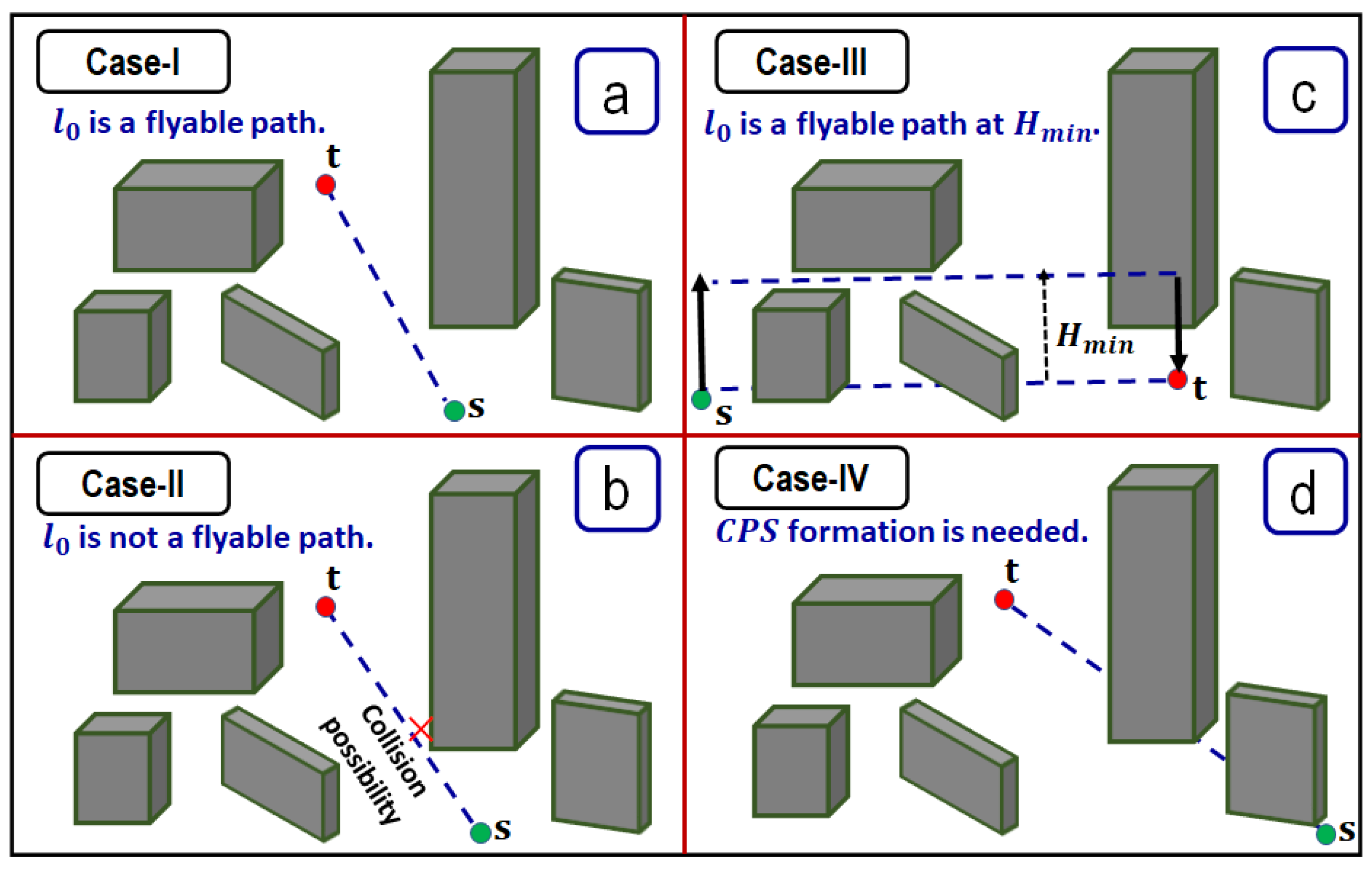After sketching the $\overline{l_o}$, four outputs can be derived, which are: (I) neither penetration nor collision, (II) not penetration, but the possibility of a collision exists, (III) penetration, but all obstacles have a lower height, and the UAV can go over them safely, and (IV) both penetration and collision. All four results are demonstrated in Figure 3.

If the $\overline{l_o}$ does not collide with any obstacle, and the collision possibility is zero, then path $P=\overline{l_o}$, which is an optimal path (e.g., a straight line) as given in Figure 3a. Moreover, if the $\overline{l_o}$ does not penetrate any obstacles, but there remain some obstacles in close proximity to the $\overline{l_o}$ with which the UAV could collide with a higher probability, then we deal with these obstacles to generate a safe P, as demonstrated in Figure 3b. In the third case, as given in Figure 3c, few obstacles are penetrated by the $\overline{l_o}$, all obstacles have a lower height, and the UAV can go over them safely. In the fourth case, as given in Figure 3d, some obstacles are penetrated by the $\overline{l_o}$, and we need to bypass them at a lower cost to find a P between s and t while fulfilling the stated objectives. Such obstacles are extracted from the map and utilized for pathfinding from the CPS. The complete pseudo-code utilized for extracting pertinent obstacles is illustrated in Algorithm 1. In Algorithm 1, map W encompassing N distinct obstacles, s, and t, are given as input. The set E, where (E⊆N) of the pertinent obstacles is retrieved as output. Line 2 can do $\overline{l_o}$ sketching between s and t. Lines 3–7 can do obstacles’ extraction that are crossed by the $\overline{l_o}$. At the end, set E of pertinent-obstacles is collected. Moreover, if no intersection occurs between the obstacles and the $\overline{l_o}$, and, then, $E=\varnothing$ will be the output.

After getting set E of pertinent obstacles, we enlarge the obstacles by a safe distance ($d_{safe}$), and apply the flying minimum and maximum limits, denoted as $h_{min}$ and $h_{max}$, respectively. Subsequently, we analyze the pertinent obstacle cross sections that are on the $\overline{l_o}$ between s and t. Then, we draw a bottom boundary, ${\Omega }_b$, around the bottom vertices of the pertinent obstacles, and a top boundary, ${\Omega }_t$, from minimal height h with path guarantees keeping s and t as two endpoints. This forms a 3D constrained space where the shape can resemble a 3D polygon, and we call this constrained region the CPS, represented with $S_1^3$. This CPS converts the more difficult problem of UAV pathfinding into the relatively easier problem of pathfinding for a 3D point. A visual overview of $S_1^3$ is demonstrated in Figure 4. The $S_1^3$ can be simply defined as full map W partitioned into a small space/region where the outline is the same as a 3D polygon, with s and t as two endpoints. It is obtained by drawing a boundary around the outermost vertices of the pertinent obstacles in such a way that a path can be found from it regardless of its quality. The process of transforming a full map into $S_1^3$ is given in Figure 4a–c. In Figure 4a, environment map W is shown, which will be converted into $S_1^3$. Figure 4b shows the $\overline{l_o}$ drawing, and identifies the corresponding pertinent obstacles (e.g., yellow obstacles) that were crossed by it; these obstacles will be used to subsequently generate $S_1^3$. Figure 4c shows the outline of $S_1^3$ in 2D form that is obtained by drawing a boundary around obstacles identified in Figure 4b as a consequence of $\overline{l_o}$ penetration.

Algorithm 1: Extracting pertinent obstacles from a 3D obstacle map.

Input     :(i) Environment map W with N distinct obstacles                   (ii) Starting location (s)                   (iii) Ending location (t)   Output   :Pertinent obstacles’ set E   Procedure:  1  Initialize, E = ∅ 2  Sketch straight line $\overline{l_o}$ between (s) and (t) // Assuming case IV given in Figure 3 3     for every obstacle $O_j$, beginning from $O_j$ = $O_1$ to the $O_n$ ∈ N do 4      if CROSSES ($\overline{l_o}$, $O_j$) then 5         $E=E\cup \left\{O_j\right\}$ 6      End if 7   End for 8 return E

The CPS can enclose the pertinent obstacles—just part of them or as a whole. In some cases, due to complex 3D environments, $S_1^3$ can enclose obstacles that do not belong to set E but that are part of $S_1^3$, either partially or completely, and we include such obstacles in E and utilize them in pathfinding. The essence of $S_1^3$ is that it guarantees a flyable path between s and t. However, $S_1^3$ may or may not be an ideal choice for a good-quality path (e.g., optimal or quasi-optimal) due to several complexity parameters (as illustrated in Figure 1) about obstacles. By considering such potential complexity parameters and a probabilistic analysis of optimal paths, we conducted a CPS complexity analysis leveraging six complexity parameters (also known as complexity constraints), prevailing in $S_1^3$ that relate to the obstacles’ geometries, and a low-cost path tends to lie outside $S_1^3$, in most cases, with a significantly higher probability.

3.3. Determining and Analyzing the Constrained Polygonal Space Complexity Using a Multicriteria-Based Method

In order to check whether $S_1^3$ is good enough for optimal/quasi-optimal pathfinding or not, we performed a multi-criteria–based complexity analysis of $S_1^3$ using multiple complexity parameters before task modeling and pathfinding. We computed the complexity, $\chi$, of $S_1^3$ by leveraging detailed information regarding the obstacles’ geometries. We employed six complexity parameters: the proportion of free spaces, the obstacle occupancy in distinct regions of the CPS, the complexity of obstacle–avoidance options, the proportion of connected obstacles, the length deviations from the optimal path, and obstacles’ tendency in the CPS that hinders the solution quality. Through extensive simulations and analysis, it is found that there exists a very firm relationship between the complexity parameters of the CPS and path quality. The total $\chi$ is the weighted sum of six parameters cited above. Brief overviews of those six complexity parameters, with their procedures and equations, are described below.

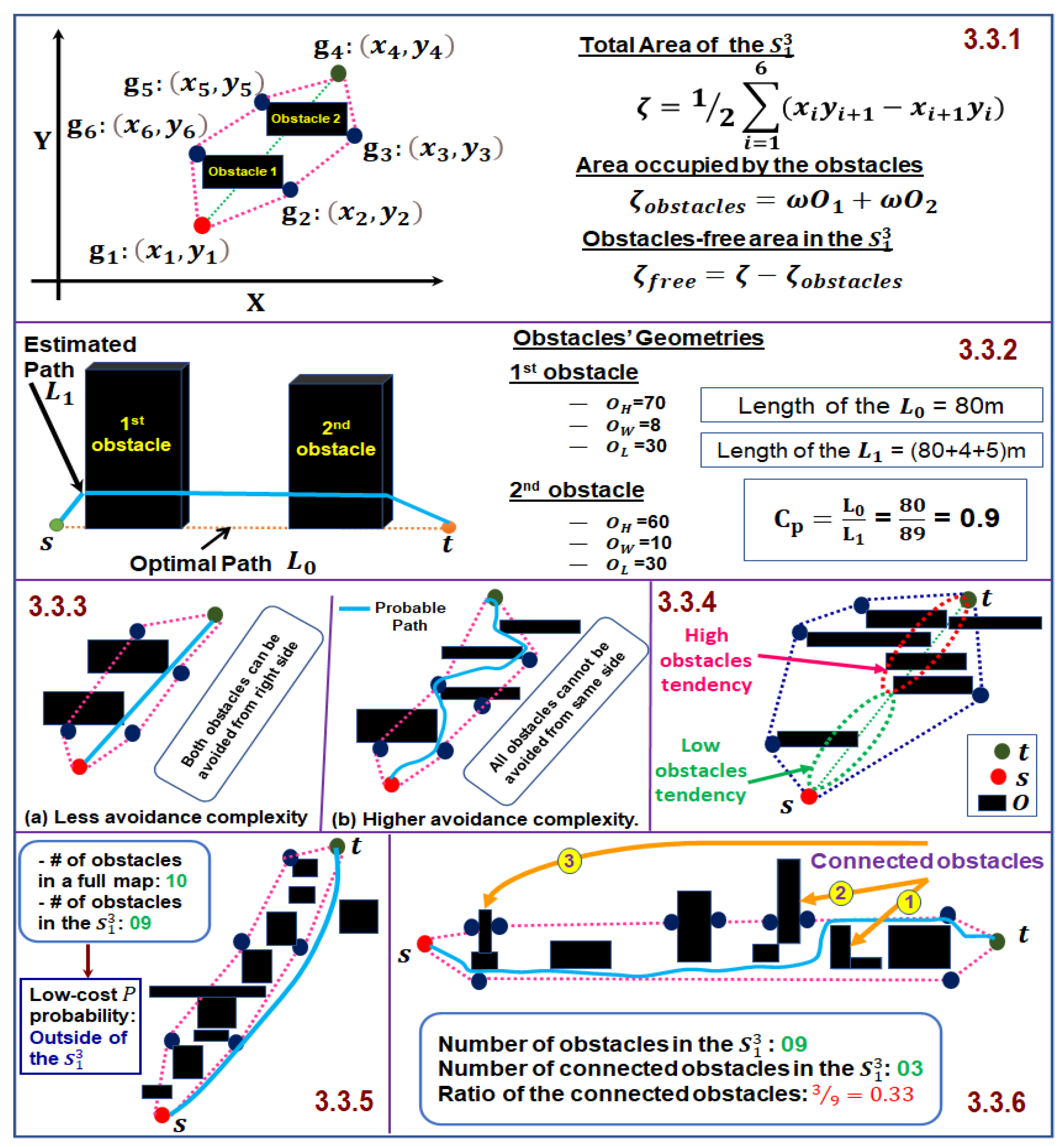
3.3.1. Free Spaces’ Ratio

To compute a feasible, safe, and smooth P, it is highly enticing that the amount of free spaces must be high in the CPS. To measure the obstacle-free spaces in the CPS, we first determine the size ($\xi$) of the $S_1^3$, blocked-spaces (${\xi }_{obstacles}$), and free-spaces (${\xi }_{free}$). The overall size ($\xi$) of the CPS that is in the form of a polygon can be obtained by the Gauss determinant using Equation (1):

$$\xi =\frac{1}{2}\sum _{i=1}^{\left|g\right|}(x_i{y}_{i+1}-x_{i+1}{y}_i)\times h$$

(1)

where $x,y$ are the coordinate values of the CPS boundary, $\left|g\right|$ denotes total vertices of the CPS boundary, and h is the height of the CPS. Out of the $\xi$-sized CPS, we find the amount occupied by the obstacles (${\xi }_{obstacles}$) using Equation (2):

$${\xi }_{obstacles}=\sum _{i=1}^n\omega O_i$$

(2)

where n denotes total obstacles’ count present in a $S_1^3$ and $\omega O_i$ denotes the obstacles’ occupancy. The occupancy of an $O_i$ obstacles can be determined using Equation (3):

$$\omega O_i=O_H\times O_L\times O_W$$

(3)

where $O_W$, $O_H$, $O_L$ denote the width, height, and length of an obstacle, respectively. The free space ($X_{free}$) amount, where UAV can fly safely, can be determined using Equation (4):

$${\xi }_{free}=\xi -{\xi }_{obstacles}$$

(4)

The ratio ($r_f$) of the free spaces can be calculated using Equation (5):

$$r_f=\frac{{\xi }_{free}}{\xi }$$

(5)

The value of $r_f$ ranges between 1 and 0. We represent this ratio as ($1-r_f$) to compute the occupied spaces value in overall CPS $S_1^3$ complexity computation.

3.3.2. Deviation in Length from an Optimal Path

The proposed method is a global PP approach, and all information about the obstacles geometries is known in advance. By utilizing the obstacles geometry information, we can estimate the path length without calculating the actual path. We estimate length of an optimal path $L_o$, where $L_o=\overline{l_o}$ as an optimal path and estimate the deviation in it that can occur due to obstacles that are on $\overline{l_o}$. We call it deviation $D^{{}^{\prime }}$ from the optimal path and formalization used to estimate is explained below.

• Computing the optimal path $L_o$ that is a straight line between s and t using Equation (6).

  $$L_o=\sqrt{{(x_t-x_s)}^2+{(y_t-y_s)}^2+{(z_t-z_s)}^2}$$

  (6)
• Calculating the deviation $D^{{}^{\prime }}$ in optimal path $L_o$ due to the presence of obstacles on the $\overline{l_o}$ between s and t locations. The D in the paths length due to an obstacle (e.g., $O_i$) is calculated using Equation (7).

  $$D_i=min(\frac{O_W}{2},O_H)$$

  (7)
• Estimating the total deviation $D^{{}^{\prime }}$ that can likely occur due to the presence of the obstacles between s and t in the CPS using Equation (8).

  $$D^{{}^{\prime }}=\sum _{i=1}^n{D}_i$$

  (8)
• Calculating the length of the estimated paths ($L_1$) avoiding all obstacles that are on the $\overline{l_0}$ using Equation (9).

  $$L_1=L_o+\sum _{i=1}^n{D}_i$$

  (9)

  where $L_1$ denotes the lengths of the paths avoiding obstacles in the selected space, $L_0$ denotes the Euclidean distance between s and t locations, n represents obstacles’ strength in the selected space, and $D_i$ denotes the degradation in path length due to obstacles.
• Computing the complexity $C_p$ of the estimated path that can assist in analyzing the $S_1^3$ complexity using Equation (10):

  $$C_p=\frac{L_o}{L_1}$$

  (10)

The value of the $C_p$ ranges between 1 and 0. We use this value to represent the estimated path complexity in terms of length in overall CPS $S_1^3$ complexity evaluation in Equation (20).

3.3.3. Complexity of the Obstacles’ Avoidance Options

There are usually four options in total to bypass any obstacle present in a W such as right, left, up, and down (in the case of hanged obstacles or flying obstacles). Meanwhile, after the space reduction, the number of options to avoid obstacle will likely be reduced, and there can be an increase in the complexity of remaining options. Because of this, a path may be taut and path length can be prolonged. Hence, while determining the CPS complexity, we take into account the complexity of options needed to bypass obstacles. To calculate the complexity ($C_{AO}$) of each option, the entropy concept is employed. Entropy is acknowledged as the most effective and accurate measurement for similar tasks in numerous fields. In this work, we consider the urban environment; therefore, the P cannot go beneath the obstacles since bottom height of each obstacle is zero, and, hence, there are only three options in total to avoid any obstacle. The strategy below is employed to calculate the $C_{AO}$.

• Find the proportion ($p_i$) value of every avoidance option (i.e., $A{O}_l$, $A{O}_r$, $A{O}_t$) category using Equation (11).

  $$p_i=\frac{A{O}_i}{b}$$

  (11)

  where b denotes the total $AO$, and its value can be determined using Equation (12).

  $$b=\sum _{i=1}^{3}A{O}_j$$

  (12)
• The complexity $C_{AO}$ of avoidance options can be calculated using Equation (13):

  $$C_{AO}=-\sum _{i=1}^b{p}_{i}lo{g}_2{p}_i$$

  (13)

The normalized value of the $C_{AO}$ lies between 0 and 1, denoted as $C_{AO}\in [0,1]$. The $C_{AO}$ with 0 value means that avoidance complexity is low (e.g., all obstacles can be avoided from the same side). In contrast, the $C_{AO}$ value 1 means that enough variations exist in options to avoid all obstacles, and the path can contain many turns. In the CPS analysis, we take into account the $C_{AO}$ values.

3.3.4. Occupancy of Obstacles at Distinct Regions of the CPS

Besides the other complexity parameters described earlier, another important parameter that can lead to genuine performance concerns while pathfinding is the obstacles’ occupancy at distinct regions of the CPS. If obstacles in large numbers are clustered at one location (e.g., obstacles’ placement in the CPS is uneven), then the path quality likely degrades. The obstacle occupancy at one place introduces cycles/sharp-turns in a P because the P revolves around boundaries of many obstacles before approaching t. To calculate occupancy ${\Pi }_o$ of obstacles, we partition $S_1^3$ into n sub-spaces $\{s_1,s_2,s_3,\cdots ,s_n\}$ and find the obstacles occupancy in each subspace $s_i$. The obstacles’ occupancy in a $s_i$ subspace can be determined by taking the ratio of the obstacles’ occupancy ${\xi }_{obstacles}$ in the $s_i$ divided by overall obstacles’ occupancy in the CPS. To calculate occupancy, the $S_1^3$ is partitioned in five equal-size sub-spaces. The occupancy ${\Pi }_{o_i}$ of the $s_i$ can be mathematically expressed as

$${\Pi }_{o_i}=\frac{s_{obstacles}^i}{{\xi }_{obstacles}}$$

(14)

where ${\xi }_{obstacles}$ denotes occupancy of all obstacles in total from the CPS as given in Equation (2) and $s_{obstacles}^i$ represent the $ith$ subspace’s obstacles occupancy, and its value can be computed using Equation (15):

$$s_{obstacles}^i=\sum _{i=1}^{O^{{}^{\prime }}}\omega O_i^{{}^{\prime }}$$

(15)

where $\omega O_i^{{}^{\prime }}$ represents an obstacle’s volume, and $O^{{}^{\prime }}$ denotes all obstacles count in the CPS. After computing the occupancy of five sub-spaces, we determine the overall occupancy ${\Pi }_o$ of the $S_1^3$ using the following equation:

$${\Pi }_o=max\{{\Pi }_{o_1},{\Pi }_{o_2},{\Pi }_{o_3},\cdots ,{\Pi }_{o_n}\}$$

(16)

where ${\Pi }_o$ is the obstacles’ occupancy in the $S_1^3$. The rationale to choose maximum values is to effectively deal with the worst cases. The occupancy analysis assists with finding the smooth paths by giving considerable attention to the regions of high occupancy.

3.3.5. Ratio of Obstacles’ Tendency in the CPS

In some scenarios, the CPS can enclose more obstacles compared to the W (e.g., the tendency of obstacles on $\overline{l_o}$ is high compared to the whole W). Hence, it is viable to assess the impact of obstacles’ tendency to yield a good quality path. To analyze the obstacles’ tendency $T_o$, we find the number of obstacles in a CPS, and take a ratio with the obstacles’ count present in a W. We denote the number of obstacles present in the CPS with n and number of obstacles present in a full map with N, respectively. We determine the value of $T_o$ using Equation (17):

$$T_o=\frac{n}{N}$$

(17)

The value of $T_o$ can lie between 0 and 1, $T_o\in [0,1]$. The higher value of $T_o$ means that more obstacles are present in the CPS. In our work, we take into account the $T_o$ value while determining and analyzing the complexity of the $S_1^3$.

3.3.6. Ratio of the Connected Obstacles

In some cases, some obstacles exist that are not directly penetrated with $\overline{l_0}$, but they have connections with the pertinent obstacles (e.g., obstacles directly crossed with $\overline{l_0}$). These obstacles can escalate the time of path computation and yield unnecessary turns in the path. Hence, while analyzing the CPS complexity, it is paramount to take into account the connected obstacles’ effect along with other five complexity parameters. The ratio of the connected obstacles can be found by counting the connected obstacles in the CPS divided by the obstacles’ count in the $S_1^3$. The count of connected obstacles can be determined using Equation (18):

$$n^{{}^{\prime }}=\sum _{j=1}^n(O_j\cup O_{CON})$$

(18)

where $O_j$ is the pertinent obstacle, and $O_{CON}$ denotes the connected obstacle with $O_j$ (e.g., pertinent obstacles). The overall ratio of the connected obstacles ($r_{co}$) can be computed using Equation (19):

$$r_{co}=\frac{n^{{}^{\prime }}}{n}$$

(19)

where $n^{{}^{\prime }}$ represents connected obstacles’ strength, and n shows the number of obstacles in E.

When all six complexity parameters’ values have been calculated, the total complexity $\chi$ of the $S_1^3$ can be quantified using Equation (20):

$$\chi \left(S_1^3\right)=w_1\times (1-r_f)+w_2\times C_p+w_3\times C_{AO}+w_4\times {\Pi }_o+w_5\times T_o+w_6\times r_{co}$$

(20)

In Equation (20), $1-r_f$ denotes the ratio of spaces occupied by obstacles, $C_p$ denotes the deviation in path length from an optimal path, $C_{AO}$ means the complexity of options while avoiding obstacles, ${\Pi }_o$ is the occupancy of the obstacles at the distinct region of the CPS, $T_o$ denotes the tendency of obstacles in the CPS in relation to a full map, and $r_{co}$ denotes the ratio of connected obstacles. The drawing of all six complexity parameters described in prior subsections (e.g., Section 3.3.1, Section 3.3.2, Section 3.3.3, Section 3.3.4, Section 3.3.5 and Section 3.3.6) is given in Figure 5.

For calculation simplicity, we used complexity parameters values in normalized form; therefore, the $\chi \left(S_1^3\right)$ ranges between 0 and 1. In Equation (20), $w_i$, where $i=1,2,3,4,5,6$ represents each complexity parameter’s weight, and they fulfill two conditions, (i) $w_1+w_2+w_3+w_4+w_5+w_6=1$, and (ii) $w_i>0$. We adjust each parameter weight by taking into account the significance and influence of every parameter in the CPS complexity analysis. The probability $\sigma$ of a path P to be found from the $S_1^3$ with good quality is given as follows:

$$\sigma \left(P\right)=\left\{\begin{array}{cc}1,\hfill & \mathrm{if}0<\chi \left(S_1^3\right)<T.\hfill \\ 0,\hfill & \mathrm{otherwise}.\hfill \end{array}\right.$$

(21)

where $\chi \left(S_1^3\right)$ represents the complexity of the $S_1^3$, and T denotes a threshold. If $\sigma \left(P\right)=1$, no extension of space is required because $S_1^3$ is appropriate for low-cost pathfinding. Meanwhile, if $\sigma \left(P\right)=0$, then an additional space will be needed to find good quality paths. The threshold T value relies on numerous global factors of the W, and local constraints (e.g., related to the UAV). In simulations, we set the threshold value to 0.7 to make a decision about the space expansion. We did substantial experiments to validate the T value using P’s length as a main criteria. However, T’s value can be tuned flexibly based on the UAV’s workspace and resources.

3.4. Expansion of the First Constrained Polygonal Space

Although $S_1^3$ always finds path P, it does not guarantee the quality of P in each scenario due to higher complexity in the obstacles. To circumvent this issue and ensure consistent quality for P in each scenario, the scenarios that require a bigger space are identified carefully through the CPS complexity analysis utilizing the six different parameters. With the assistance of the complexity analysis of $S_1^3$, for a good-quality P, we can accurately identify the cases that require relatively more space than already in $S_1^3$. Having sufficient information about the obstacles connected with the boundary of $S_1^3$ enables us to flexibly expand the space to the next level. We adopted this method to expand the space, since it yields less computing overhead and significantly enhances path quality. Hence, by processing obstacles that are penetrated by the boundary of $S_1^3$, and by marking a polygonal boundary in an analogous way, the first CPS formation emanates into a second CPS of a relatively bigger size, compared to the $S_1^3$ as visually depicted in Figure 6b.

We denote this expanded space with $S_2^3$, and it encompasses $S_1^3$ fully. The $S_2^3$ includes pertinent obstacles fully, and it provides greater opportunities for P to be determined from $S_2^3$ solely. The utility of the $S_2^3$ is that it is highly desirable space for producing P of shortest lengths. The space can be extended to nested levels in identical manner. Meanwhile, we expand the spaces only up to 2-levels because an optimal/quasi-optimal P tends to lie in $S_1^3$ and $S_2^3$ with acceptable probability. After the selection of appropriate highest priority space, an ESWG is constructed for pathfinding.

3.5. Extremely Sparse Waypoint Graph Generation from the Selected CPS

Waypoint graph (WG) is one of the approaches for task modeling and pathfinding, respectively. The WG constructs an indirect and compact graph connecting s with t by catching the connectivity of the ${\xi }_{free}$ to form a multiple paths’ network. However, generating a WG is very expensive in terms of computation. The overall time complexity of generating a WG with n nodes is $O\left(n^3\right)$. Many studies that have focused on lowering the complexity of the WG generation have been reported by joining adjacent obstacles, altering obstacles’ shape, and ignoring small obstacles. More recent research [60] highlights that WG’s time complexity in the 3D environments can be decreased to the $O\left(n^2\right)$ by only considering the obstacles crossed by the $\overline{l_o}$. To expedite the time complexity reduction of the WG, this paper suggests a new concept of an ESVG construction method which does not compose a dense WG. This method forms an ESVG from the CPS like a roadmap with connectivity between s and t through intermediate nodes. An ESVG is a double-edge type graph G of reachable and mutually-visible locations, mathematically expressed as: $G=\{X,Y\}$.

To construct a G from the 3D CPS, two steps are generally applied: making a nodes’ set X and generating an edge set Y. The initial step is about creating nodes set X. We utilized three vertices of obstacles, bottom, top, and mid to make an ESWG for the first time. Both bottom and top vertices’ geometry values are known, and mid vertices can be found leveraging the midpoint formula on top and bottom axis values. Every obstacle has total eight vertices (e.g., four bottom and four top). An $ith$ obstacle’s vertices and their respective values can be expressed mathematically in a matrix as demonstrated in Equation (22). The height of bottom four vertices of each obstacles are transformed to the $h_{min}$ and top vertices of the obstacles have the same height as of the CPS height (e.g., h). In below metrics, the value of $z_{min}$ is zero but after adjustment becomes $h_{min}=z_{min}$:

$$O_i=\left[\begin{array}{ccccc}{x}_{min}& y_{min}& z_{max};x_{min}& y_{min}& z_{min}\\ x_{min}& y_{max}& z_{max};x_{min}& y_{max}& z_{min}\\ x_{max}& y_{min}& z_{max};x_{max}& y_{min}& z_{min}\\ x_{max}& y_{max}& z_{max};x_{max}& y_{max}& z_{min}\end{array}\right]=\left[\begin{array}{ccccc}1131& 1632& 241;1131& 1632& 23\\ 1131& 1703& 241;1131& 1703& 23\\ 1209& 1632& 241;1209& 1632& 23\\ 1209& 1703& 241;1209& 1703& 23\end{array}\right]$$

(22)

For example, an O whose original $z_{max}$ is greater than the CPS height, and the bottom and top vertices are fully known, the pair of mid-points’ two side faces denoted with $f_1$ and $f_2$ can be determined using Equations (23) and (24), respectively:

$$f_1=\{\frac{x_{max}+x_{min}}{2},y_{min},z_{min}\},\{\frac{x_{max}+x_{min}}{2},y_{max},z_{min}\}$$

(23)

$$f_2=\{\frac{x_{max}+x_{min}}{2},y_{min},z_{max}\},\{\frac{x_{max}+x_{min}}{2},y_{max},z_{max}\}$$

(24)

A similar procedure can be utilized to find the pair of vertices around all obstacles. After computing set X from the pertinent obstacles, we add both s and t in a set X and generate set Y of edges through two novel strategies and visibility-checks. Any two nodes u and v in X are inter-visible if a $\overline{uv}$ segment of line connecting them is collision free. A function named-line-of-sight (LOS) determines the visible segments among pairs of nodes through visibility analysis. The time complexity of this mechanism heavily relies on the function of LOS checking, and number of nodes. Meanwhile, in our work, we incorporate two additional strategies of far-reachability (FR) and direction-guidance (DG), thereby time complexity is significantly reduced. In addition, it only adds the edge between a vertices’ pair that are as far as possible from each other and that guide to the t’s direction. We set the visibility to off/false using coordinate values for those pairs of vertices that are on the same obstacle but do not favor the direction of the t. Hence, the visibility checking function has less time complexity in making a G. The time complexity of an ESWG formation is the $O\left({\left(nfl\right)}^2\right)$ time, where l denotes the number of levels, n denotes obstacles’ count, and f represents the counts of obstacles’ facets. However, the upper-bound of the l is constant (e.g., $l=3$ ); therefore, ESWG’s time complexity is $O\left({\left(fn\right)}^2\right)$. With the help of X and Y, a G is obtained that has reliable connectivity between s and t, and it encompasses all characteristic of a roadmap.

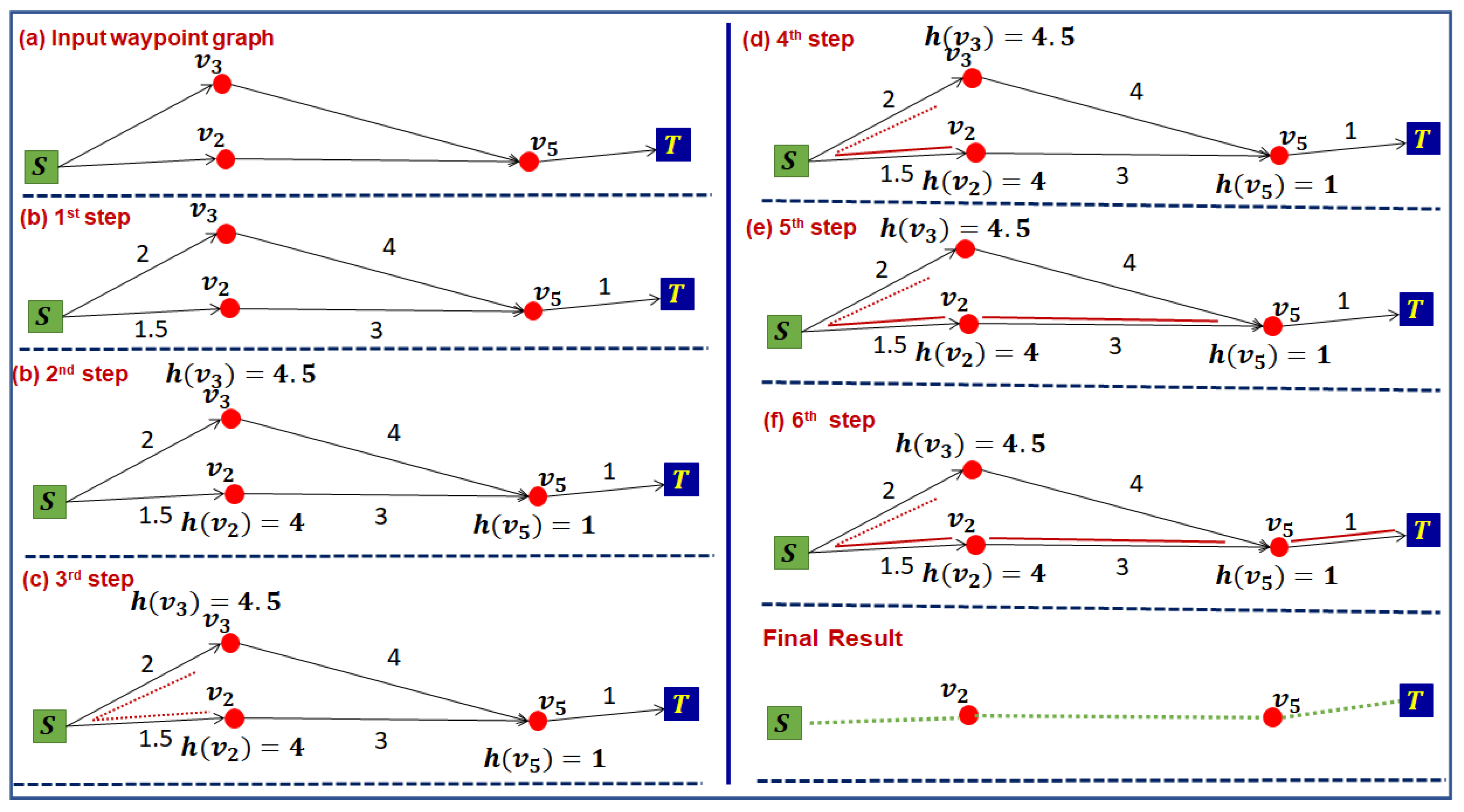
3.6. Path Finding from an ESWG and Enhancing Obtained Path Quality

Once an ESWG is modeled, a path searching algorithm is employed to search a P from it. In this paper, we used $A^{*}$ algorithm for computing a P between s and t from an ESWG. The A* is reliable algorithms for extracting a P of low-cost. The evaluation function utilized by this algorithm is expressed in Equation (25):

$$f\left(n\right)=g\left(n\right)+h\left(n\right)$$

(25)

In Equation (25), the $f\left(n\right)$ denotes the estimated path cost in total between s and t via a node n, the $g\left(n\right)$ denotes the actual distance to reach node n, and the $h\left(n\right)$ is a heuristic function that computes the distance from node n to t. This algorithm was selected to make P’s computing process fast. By exploring an ESWG using this algorithm, an abstract P is found. We consider both length and time of the obtained P for evaluating its quality. Meanwhile, in some cases, the P cannot be of minimal length, which needs post-processing to shorten it. We present the working of the $A^{*}$ algorithm while finding a path between s and t in Figure 7.

In many UAV practical applications, the length of the P is paramount, and to preserve UAV resources, it should be minimum. To address this issue, we shorten P’s length by including more nodes in close proximity of it, and refine the sharp turns. The path quality improvements is mainly carried out by determining the adjacent P’s neighbor nodes, find the proximity between the adjacent neighbor nodes and P nodes, and in the close proximity of the P, we introduce new nodes with relatively denser resolution and add smooth edges. The reason to add more nodes closely is to retain visibility to improve P quality. After injecting additional nodes, a P of good quality is obtained by jointly using the newly added and the P nodes. This path-refining method has the potential to improve path quality significantly with reduced computing cost.

4. Results and Discussion

This section explains the simulation experiments and corresponding results. The performance of the proposed PP method was analyzed using two criteria: time complexity and path length compared to prior studies. To make the proposed PP method a benchmark, we compared the simulation results with randomized motion planning and visibility graph–based algorithms. The simulation tests were performed and compared using Matlab v. 9.8.0.1451342 (R2020a) on a computer running Windows 10 with 8 GB of RAM and a 2.6 GHz CPU. In the tests, we assumed a 25 kg fixed-wing UAV similar to ones used in existing studies. We took into account both global and local constraints in the simulations. The parameters of the local constraints (i.e., on the UAV) were a 1 m wingspan and a maximum turning angle at a radius of $\pi /6$ . The minimum and maximum flying altitudes were $h_{min}=23$ m, $h_{max}=155$ m. The global constraints belonged to the geometry of obstacles in W. We consider six complexity parameters that can significantly hinder the quality of a P and the UAV’s safety while selecting a space size. We assumed that the UAV had enough battery power to complete the task in one flight. The safe distance to avoid collisions with obstacles was $10m$ ($d_{safe}=10$ m). We assumed that wind was negligible during the flight. The proposed method finds P using an ESWG that respects both global and local constraints. The weights of space complexity parameters were $w_1=0.2$, $w_2=0.1$, $w_3=0.2$, $w_4=0.2$, $w_5=0.1$, and $w_6=0.2$. We assigned values to these weights by considering the significance and influence of each parameter on the accurate space selection for an optimal/quasi-optimal pathfinding. We tested our method with diverse combinations of the weight values, and analyzed the accuracy of space selection for optimal/quasi-optimal paths. Subsequently, we determined the best combination of these weight indexes’ values that make accurate space selection consistently. Furthermore, these weight values were validated via numerical analysis by computing optimal paths from numerous maps using whole W, and analyzing the number of times optimal paths tend to lie in the selected space. The locations for s and t were chosen randomly during experiments. We compared our PP method’s performance with two existing algorithms: the ApVL algorithm proposed by Guillermo et al. [60] and the RRT*-AB algorithm proposed by Noreen et al. [70]. Both comparison algorithms are state-of-the-art for PP. We tested them on our maps to compare the performance of our method with them. We show a sketch of the 3D maps employed in the experiments and three exemplary paths from each method in Figure 8.

The path produced by the proposed PP method was more smooth and shorter than the paths from the other methods. To analyze and compare the proposed PP method’s results, we designed three distinct scenarios with sufficient obstacles in the 3D environment maps. Each scenario was tested with all three methods, and the results were analyzed. All obstacles had a random width, depth, and height with a rectangular-shaped base. Comprehensive details on maps counts, map sizes, s and t locations, numbers of obstacles and their geometric information, etc. are given in each scenario description below.

4.1. Comparison with the Existing Approaches by Varying Map Sizes and Obstacle Counts

This scenario is defined with W at sizes ranging between 100 m × 100 m × 300 m–1000 m × 1000 m × 400 m. It encompassed 50 maps with distinct obstacle counts (e.g., 5–50). For the sake of simplicity and rational comparisons, we categorized all maps into 10 distinct groups considering both map size and obstacle strengths, as given in

Table 1. Details of the 3D maps used in simulations and comparisons of task modeling results.

Maps Group No.	3D Maps’ Sizes (in m)	Obstacles Strength	Proposed PP Method	ApVL Algorithm [60]	RRT*-AB Algorithm [70]
	($\mathit{x}\times \mathit{y}\times \mathit{z}$)	(upto 50)	Avg. Computing Time (in s)	Avg. Computing Time (in s)	Avg. Computing Time (in s)
$1.$	100 × 100 × 300	5	0.98	1.46	2.97
$2.$	200 × 200 × 300	10	5.61	8.31	16.81
$3.$	300 × 300 × 300	15	17.01	23.54	34.20
$4.$	400 × 400 × 300	20	39.28	49.52	65.21
$5.$	500 × 500 × 300	25	76.26	98.81	115.04
$6.$	600 × 600 × 400	30	100.65	111.19	141.81
$7.$	700 × 700 × 400	35	134.03	137.599	185.93
$8.$	800 × 800 × 400	40	155.01	186.29	211.11
$9.$	900 × 900 × 400	45	180.21	201.56	225.13
$10.$	1000 × 1000 × 400	50	191.25	209.25	249.55

. The locations for s and t were marked in alternate places for every test/map. Furthermore, the obstacle density in W varied on each map. The ApVL algorithm [60] processed only obstacles that were on the $\overline{l_o}$ and generated a dense graph to find P. However, the ApVL algorithm has higher complexity, and it produced a non-taut P in most scenarios due to the connected obstacles in urban environments, as shown in Figure 8b. The RRT*-AB algorithm restricts the space, but it explores many locations while finding P. The P generated by this algorithm had a longer length, and computing time was immense. In contrast, the proposed PP method processed fewer obstacles and employed an ESWG to find a P with good quality. The complete information about maps utilized in this particular scenario and the mean computing time for task modeling by our PP method and its comparisons with the two previous algorithms are given in Table 1.

The computing time for modeling the UAV environment shown in Table 1 is the total time needed to constrain the space, an ESWG construction, and an ESWG’s expansion for path-quality improvements. From Table 1, we can see that time surged with an increase in the map size and obstacle counts. Through extensive comparisons with prior PP algorithms, our method lowered computing time for task modeling by 15.05% on average. The pathfinding results (i.e., time needed and path length) and their comparisons with the two existing algorithms are depicted in Figure 9.

Both computing time and path length are the mean of five maps in each map’s group (given in Table 1) with arbitrary obstacles’ placement. The simulation results emphasize that, for each method, there is a surge in the computation time with the increase in W’s complexity. Moreover, the proposed PP method shows 15.4% and 33.6% curtailment in mean computing time compared to the ApVL algorithm and the RRT*-AB algorithm, respectively. In path lengths, the proposed method shows 5.34% improvements compared to the ApVL algorithm. Moreover, average improvements in the path lengths compared to the RRT*-AB algorithm are 6.34%. These results highlight that the proposed PP method is superior in terms of both computing time and path length over prior algorithms.

4.2. Comparison with the Existing Approaches by Varying the Number of Obstacles

This scenario is comprised of 10 maps with varying numbers of obstacles in a W of 1 km${}^2$ to analyze the impact on our PP method’s performance from increasing the number of obstacles. The obstacles were clustered between s and t in such a way that all methods would avoid them during pathfinding. Figure 10 presents the results of our proposed PP method and a comparison with the other algorithms from varying the number of obstacles. When W enclosed more obstacles, the suggested method could quickly determine a good-quality and safe P from W. It was better than the ApVL and RRT*-AB algorithms, based on the metrics, even when varying the number of obstacles in the CPS. The P determined by the proposed method was the shortest and smoother than the other two algorithms. Through simulation results and their comparison with previous methods on 10 obstacles’ counts-based maps, the proposed method decreased the computing time for pathfinding by $27.06\%$, on average. For path lengths, the paths generated by our PP method, on average, were $4.6\%$ shorter (i.e., produced at a lower cost) than the previous methods.

4.3. Comparison with the Existing Approaches by Varying Source and Target Locations

This scenario was tested using a W at 150 m × 150 m × 400–1000 m × 1000 m × 400 m. It encompassed five maps with obstacle counts of up to 25. We analyzed our method’s performance through seven runs on every map with different coordinates for s and t in each run. By varying the positions of s and t, the number of obstacles to be modeled in each run/test can be distinct, and, accordingly, comparison metrics can vary with W complexity. The proposed method’s averages, obtained from the seven runs on each map, are given in

Table 2. Proposed method pathfinding results’ comparison with the ApVL and the RRT*-AB algorithms.

Maps Sizes (m)/Obstacles’ Count	ApVL Algorithm [60]		RRT*-AB Algorithm [70]		Proposed PP Method
	Avg. Time (s)	Avg. Path Length (m)	Avg. Time (s)	Avg. Path Length (m)	Avg. Time (s)	Avg. Path Length (m)
150 × 150 × 400/5	0.35	305.4	0.61	295.91	0.26	300.14
400 × 400 × 400/10	0.55	620.12	0.75	650.75	0.47	599.27
600 × 600 × 400/15	0.74	860.51	0.96	900.90	0.59	800.05
800 × 800 × 400/20	0.98	1020.01	1.81	1050.05	0.75	990.5
1000 × 1000 × 400/25	2.45	1100.05	2.75	1120.75	1.52	1070.21

. The results indicate that the proposed method yielded comparable performance in all tests.

The proposed method yielded an average computing time of 0.71 s, compared to the ApVL and RRT*-AB algorithms, which had mean computing times of 1.01 s and 1.37 s, respectively. In addition, the proposed method lowered the path length, compared to both prior algorithms, by 5.05%. Although the proposed method gave better results, a relatively higher number of initial P nodes can degrade its performance in complex environments. The worst-case complexity with our method was $O\left(n^3\right)$. However, the test results revealed that time complexity did not accelerate like $O\left(n^3\right)$ in all test scenarios for finding good quality paths. The results obtained from all these scenarios showed that our method performed consistently better than the ApVL and the RRT*-AB algorithms. Aside from the path lengths and computing times, we analyzed and compared its performance against prior algorithms with respect to graph/tree nodes and path node counts. In Figure 11, the results of the proposed method in terms of average path nodes and graph/tree nodes for the above experiments are presented. As shown in Figure 11, both the graph nodes and path points of our ESWG method were lessened, compared to the prior methods.

Analysis of the memory requirements: As shown in Figure 11a, the proposed PP method generates a WG with fewer vertices. In addition, it does not register visibility of the edges that contribute minimally in an optimal/quasi-optimal path due to less coverage in terms of distance or they are not in the same direction as the target location while generating an ESWG. Therefore, the memory requirements of proposed method are not high compared to the existing methods and a complete graph. However, most global PP methods keep all visible edges in the memory that significantly increase the memory requirements. Furthermore, the visibility check function is called a substantial number of times in visibility graph-based PP methods, thereby space complexity drastically increases. The proposed method resolves these space complexity related issues through reduction in search space, modeling tasks with an ESWG, producing far lower but relevant edges and vertices, and reducing the visibility checks between vertices by incorporating far-reachability and direction-guidance concepts while making an ESWG.

The proposed PP method is complete, and it can be used for many UAV practical applications in urban environments. The proposed method gives good performance due to two main concepts: (i) a new space reduction concept is proposed, which not only assists in lowering the time complexity by restricting the path exploration in the space of highest priority, but also assists in finding low-cost paths in most cases; and (ii) an ESWG, which models the tasks with far lower edges and vertices that curtails the computing time of path searching significantly by making a direction-guided search of the target location. It effectively resolves the trade-off between optimality and efficiency in pathfinding from an urban environment populated by various obstacles.

5. Conclusions and Future Directions

This article proposed a new PP method based on CPS and an ESWG to enable a UAV’s safe navigation in 3D urban environments. The main objectives of the proposed PP method are to lower the time complexity in both task modeling and pathfinding without degrading the path quality for UAVs operating at lower elevations in urban environments with fixed, convex obstacles. The main contributions of this article are listed as follows:

• We propose a new PP method based on CPS and an ESWG that has the potential to find an optimal/quasi-optimal path with considerably reduced time complexity.
• We propose a new space reduction method that abstracts the full map into a 3D constrained polygonal space that guarantees a path for the UAV’s mission.
• We analyze the effectiveness of CPS for low-cost paths considering six complexity parameters, including the ratio of free space, obstacle density in distinct regions of the CPS, the complexity in the options for avoiding obstacles, deviation in the length from the optimal path, the ratio of connected obstacles to pertinent obstacles, and obstacle tendencies in the CPS.
• The proposed method enlarges the CPS to the next level/space by including obstacles that are in close proximity to the first CPS if the first CPS fails to provide an opportunity for low-cost solutions owing to a higher complexity from obstacles in it.
• The proposed method generates an ESWG from the CPS, leveraging the principles of maximum distance reachability, having only a few nodes and edges, and direction guidance, and it computes an abstract path that is further improved with the assistance of more nodes and edges around it.
• This initial work makes use of obstacle information from an underlying environment in order to lower the computing overhead for pathfinding without compromising path quality in 3D urban environments.

The proposed method performance is substantiated through extensive tests, and, in most cases, it performs consistently better than prior PP methods. It lowers pathfinding time complexity considerably by restricting path exploration solely in the highest priority CPS that has the greatest chance of providing an optimal/sub-optimal path. While conducting the tests, we considered numerous parameters related to the underlying operating environment’s complexity and UAV’s safety. Meanwhile, during the PP at lower elevations in urban environments, we may need to consider hanged/thin obstacles (e.g., electrical wires and poles in the streets). Another group of evaluation parameters can be the wind/gust and wind/crosswind (e.g., wind’s direction and speed), especially when passing through buildings. Hence, further testing with these parameters is yet to be investigated in future work. Finally, we intend to analyze the fidelity of our proposed PP method with other task modeling methods (e.g., Voronoi diagrams, grids, and navigation meshes, etc.).