
Robust Approach to Supervised Deep Neural Network Training for Real-Time Object Classification in Cluttered Indoor Environment

Abstract
:1. Introduction
2. Problem Statement and Methodology
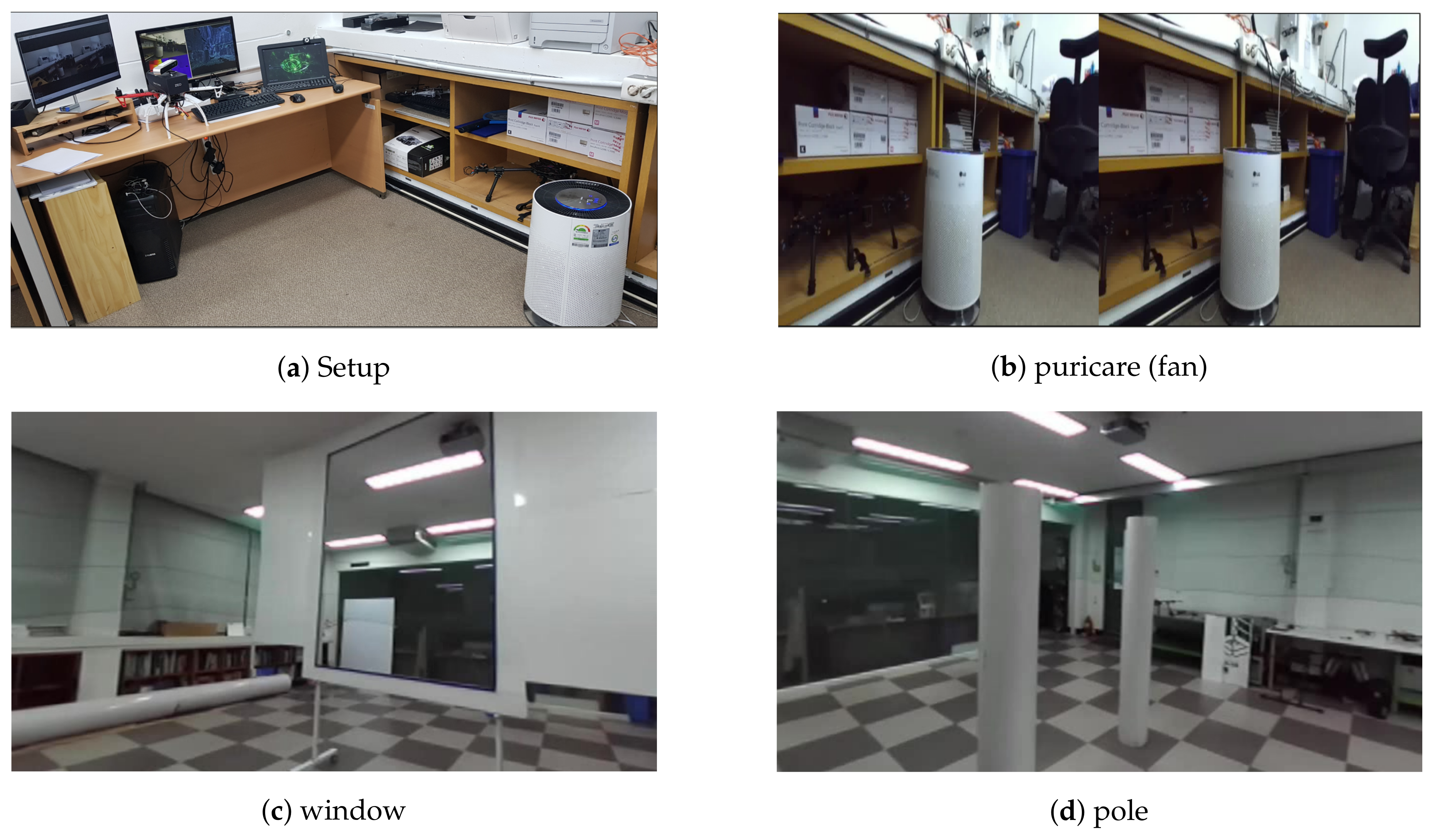
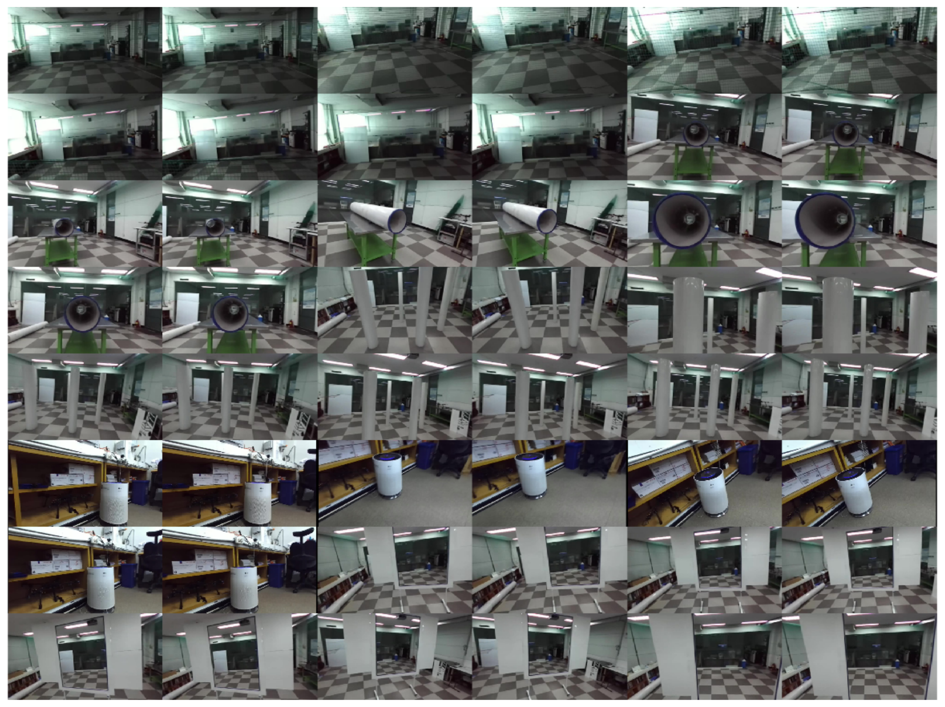
3. Data Preparation and Pre-Processing Methodology
4. Network Architecture Design
- image input layer
- convolution 2D layer
- batch normalization layer
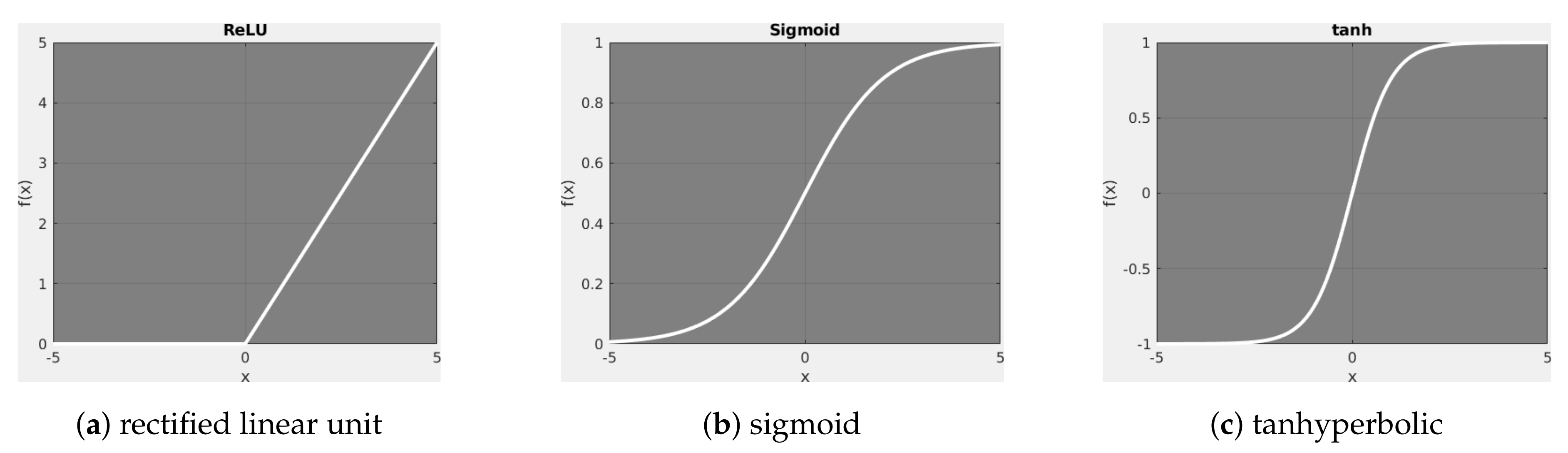
- relu layer
- max pooling 2D layer
- fully connected layer
- softmax layer
- classification layer
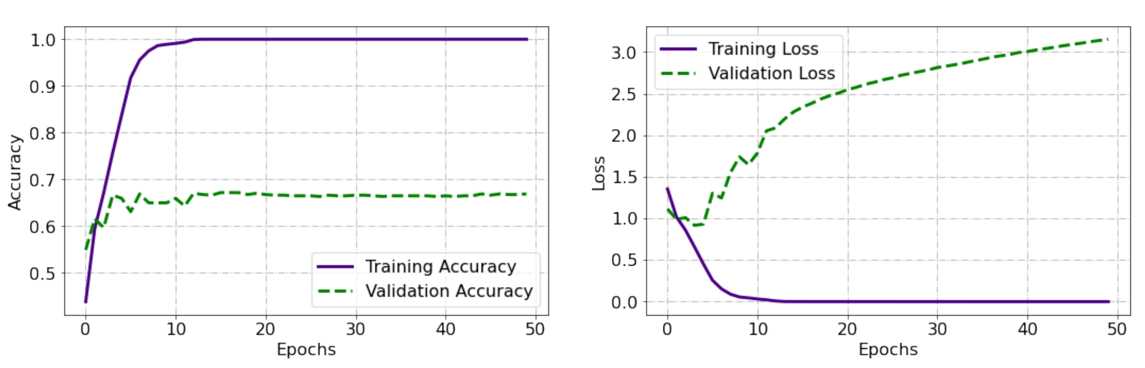
Training the Neural Network
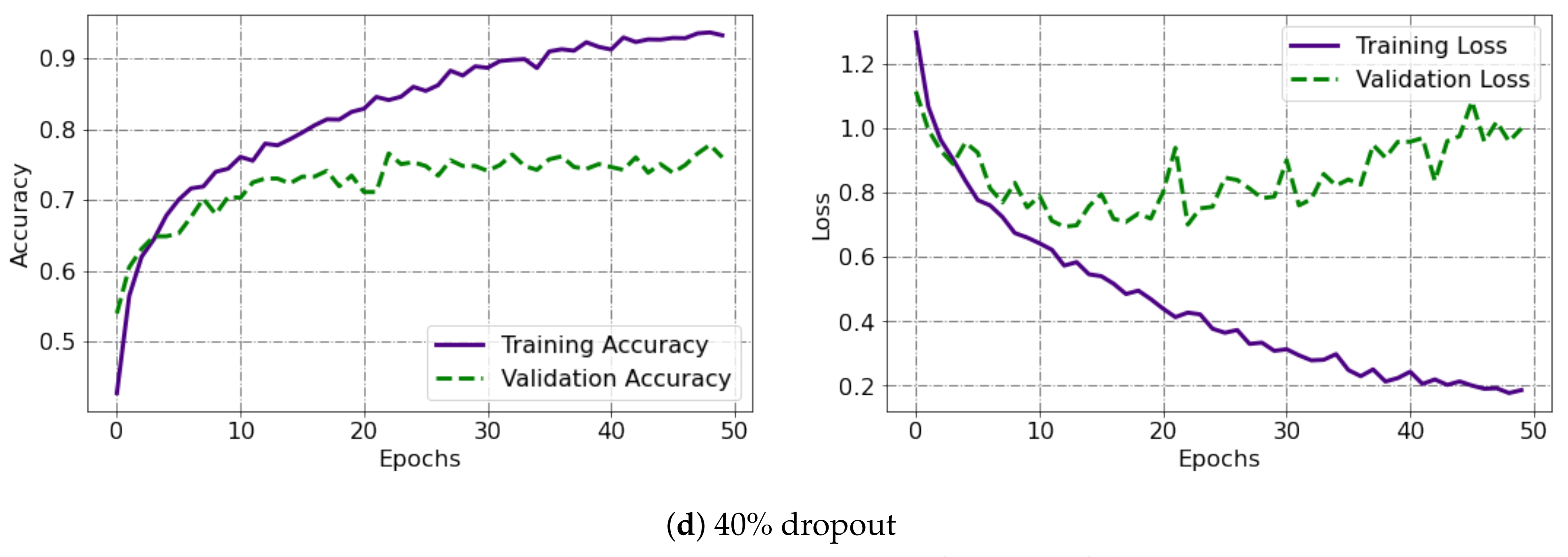
Parameter Optimization
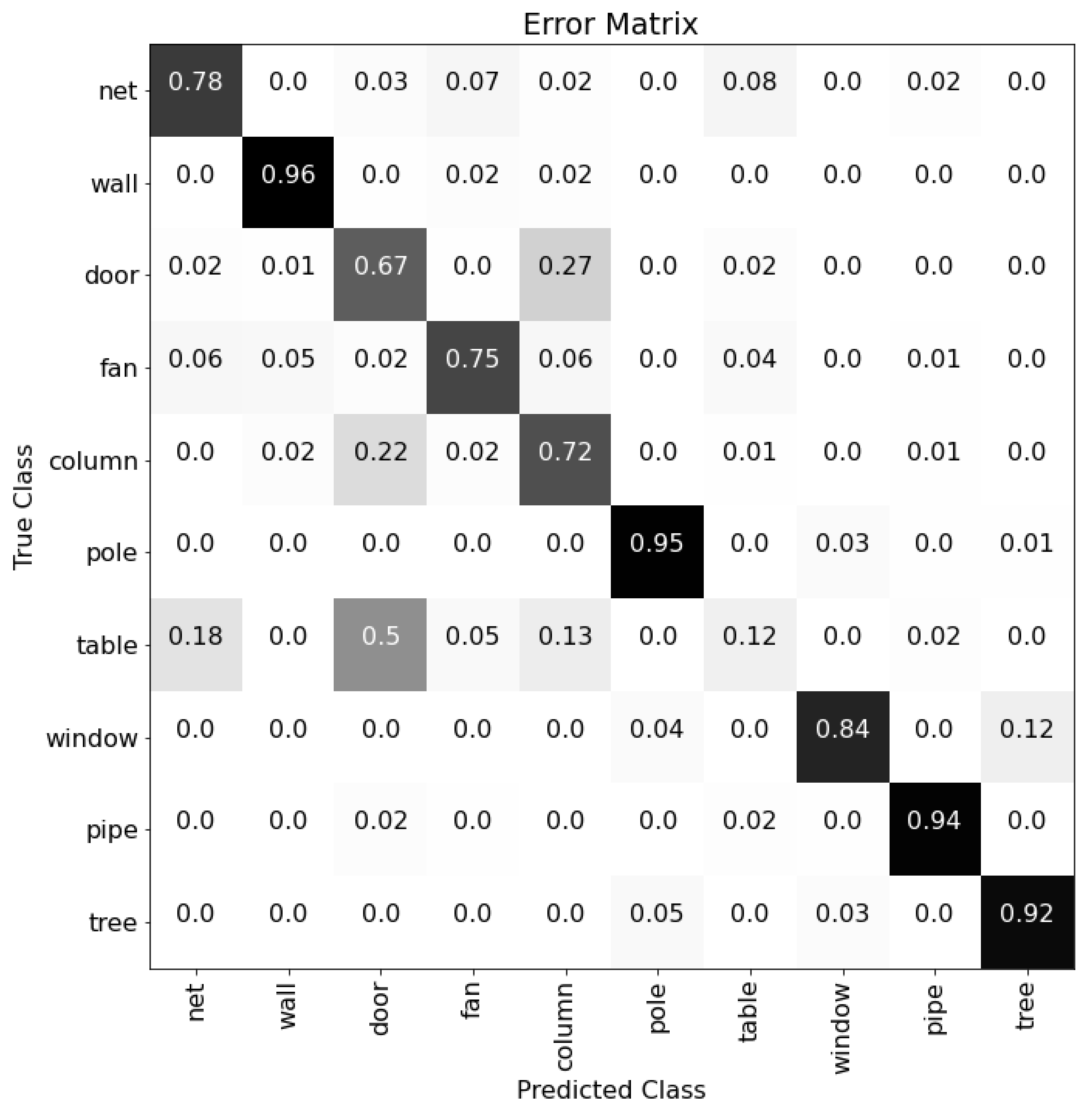
5. Results and Discussion
6. Conclusions
Author Contributions
Funding
Institutional Review Board Statement
Informed Consent Statement
Conflicts of Interest
References
- Naghavi, S.H.; Avaznia, C.; Talebi, H. Integrated real-time object detection for self-driving vehicles. In Proceedings of the 10th Iranian Conference on Machine Vision and Image Processing, Isfahan, Iran, 22–23 November 2017. [Google Scholar]
- Liu, D.; Cui, Y.; Chen, Y.; Zhang, J.; Fan, B. Video object detection for autonomous driving: Motion-aid feature calibration. Neurocomputing 2020, 409, 1–11. [Google Scholar] [CrossRef]
- Wang, Y.; Liu, D.; Jeon, H.; Chu, Z.; Matson, E. End-to-end learning approach for autonomous driving: A convolutional neural network model. In Proceedings of the International Conference on Agents and Artificial Intelligence 2019, Prague, Czech Republic, 19–21 February 2019. [Google Scholar]
- Saloni, W. The Role of Autonomous Unmanned Ground Vehicle Technologies in Defense Applications. Aerospace & Defense Technology Magazine. 2020. Available online: https://www.aerodefensetech.com/component/content/article/adt/features/articles/37888 (accessed on 1 April 2021).
- Niu, H.; Gonzalez-Prelcic, N.; Heath, R.W. A uav-based traffic monitoring system-invited paper. In Proceedings of the IEEE 87th Vehicular Technology Conference, Porto, Portugal, 3–6 June 2018. [Google Scholar]
- Sarthak, B.; Sujit, P. UAV Target Tracking in Urban Environments Using Deep Reinforcement Learning. arXiv 2020, arXiv:2007.10934. [Google Scholar]
- Zhen, J.; Balasuriya, A.; Subhash, C. Autonomous vehicles navigation with visual target tracking: Technical approaches. Algorithms 2008, 1, 153–182. [Google Scholar]
- Aguilar, W.G.; Luna, M.A.; Moya, J.F.; Abad, V.; Parra, H.; Ruiz, H. Pedestrian detection for UAVs using cascade classifiers with meanshift. In Proceedings of the IEEE 11th International Conference on Semantic Computing, San Diego, CA, USA, 30 January–1 February 2017. [Google Scholar]
- Gageik, N.; Benz, P.; Montenegro, S. Obstacle detection and collision avoidance for a uav with complementary low-cost sensors. IEEE Access 2015, 3, 599–609. [Google Scholar] [CrossRef]
- Zhang, W.J.; Yang, G.; Lin, Y.; Gupta, M.M.; Ji, C. On the definition of deep learning. In Proceedings of the 2018 World Automation Congress (WAC), Stevenson, WA, USA, 3–6 June 2018. [Google Scholar]
- Yann, L.; Yoshua, B.; Geoffrey, H. Deep learning. Nature 2015, 521, 436–444. [Google Scholar]
- Jurgen, S. Deep learning in neural networks: An overview. Neural Netw. 2015, 61, 85–117. [Google Scholar]
- Alzubaidi, L.; Zhang, J.; Humaidi, A.J.; Al-Dujaili, A.; Duan, Y.; Al-Shamma, O.; Santamaría, J.; Fadhel, M.A.; Al-Amidie, M.; Farhan, L. Review of deep learning: Concepts, CNN architecture, challenges, applications, future directions. J. Big Data 2021, 8, 1–74. [Google Scholar] [CrossRef]
- Jefferson, S.; Gustavo, P.; Fernando, O.; Denis, W. Vision-Based Autonomous Navigation Using Supervised Learning Techniques. In Proceedings of the 12th Engineering Applications of Neural Networks and 7th Artificial Intelligence Applications and Innovations, Corfu, Greece, 15–18 September 2011. [Google Scholar]
- Fabrice, R.N. Machine Learning and a Small Autonomous Aerial Vehicle Part 1: Navigation and Supervised Deep Learning. Tech. Rep. 2018. [Google Scholar] [CrossRef]
- Wang, D.; Chen, J. Supervised Speech Separation Based on Deep Learning: An Overview. Available online: https://arxiv.org/pdf/1708.07524.pdf (accessed on 1 April 2021).
- Yang, X.; Kwitt, R.; Niethammer, M. Fast predictive image registration. In Deep Learning and Data Labeling for Medical Applications; Springer: Cham, Switzerland, 2016; pp. 48–57. [Google Scholar]
- Louati, H.; Bechikh, S.; Louati, A.; Hung, C.C.; Said, L.B. Deep convolutional neural network architecture design as a bi-level optimization problem. Neurocomputing 2021, 439, 44–62. [Google Scholar] [CrossRef]
- Bayot, R.; Gonalves, T. A Survey on Object Classfication Using Convolutional Neural Networks. 2015. Available online: https://core.ac.uk/download/pdf/62473376.pdf (accessed on 1 April 2021).
- Thumu, K.; Gurrala, N.R.; Srinivasan, N. Object Classification and Detection using Deep Convolution Neural Network Architecture. Int. J. Recent Technol. Eng. 2020. [Google Scholar] [CrossRef]
- Rikiya, Y.; Mizuho, N.; Richard, K.G.D.; Kaori, T. Convolutional neural networks: An overview and application in radiology. Insights Imaging 2018, 9, 611–629. [Google Scholar]
- Richard, L.; Roberto, F. Space Object Classification Using Deep Convolutional Neural Networks. In Proceedings of the 19th International Conference on Information Fusion, Big Sky, MT, USA, 3–10 March 2018. [Google Scholar]
- Bai, S.; Kolter, J.Z.; Koltun, V. An empirical evaluation of generic convolutional and recurrent networks for sequence modeling. arXiv 2018, arXiv:1803.01271. [Google Scholar]
- Asifullah, K.; Anabia, S.; Umme, Z.; Aqsa, S.Q. A survey of the Recent Architectures of Deep Convolutional Neural Networks. Artif. Intell. Rev. 2020, 53, 5455–5516. [Google Scholar]
- Neha, S.; Vibhor, J.; Anju, M. An Analysis Of Convolutional Neural Networks For Image Classification. Procedia Comput. Sci. 2018, 132, 377–384. [Google Scholar]
- Karen, S.; Andrew, Z. Very Deep Convolutional Networks for Large-Scale Image Recognition. arXiv 2015, arXiv:1409.1556. [Google Scholar]
- Christian, S.; Wei, L.; Yangqing, J.; Pierre, S.; Scott, R.; Dragomir, A.; Dumitru, E.; Vincent, V.; Andrew, R. Going Deeper with Convolutions. arXiv 2015, arXiv:1409.4842. [Google Scholar]
- Alex, K.; Ilya, S.; Geoffrey, E.H. ImageNet Classification with Deep Convolutional Neural Networks. Imagenet Compet. 2012, 25, 1097–1105. [Google Scholar]
- Nielsen, M. Neural Networks and Deep Learning. Free Online Book, Michael Nielsen, 2019; Chapter 5. Available online: http://neuralnetworksanddeeplearning.com/about.html (accessed on 1 April 2021).
- Soumya, J.; Dhirendra, K.V.; Gaurav, S.; Amit, P. Issues in Training a Convolutional Neural Network Model for Image Classification. Adv. Comput. Data Sci. 2019. [Google Scholar] [CrossRef]
- Hugo, L.; Yoshua, B.; Jerome, L.; Pascal, L. Exploring Strategies for Training Deep Neural Networks. J. Mach. Learn. Res. 2009. [Google Scholar] [CrossRef]
- He, K.; Zhang, X.; Ren, S.; Sun, J. Deep Residual Learning for Image Recognition. Computer Vision and Pattern Recognition. arXiv 2015, arXiv:1512.03385. [Google Scholar]
- Stephan, Z.; Yang, S.; Thomas, L.; Ian, G. Improving the Robustness of Deep Neural Networks via Stability Training. arXiv 2016, arXiv:1604.04326. [Google Scholar]
- Tamás, O.; Anton, R.; Ants, K.; Pedro, A.; David, P.; Jan, K.; Pavel, K. Robust Design Optimization and Emerging Technologies for Electrical Machines: Challenges and Open Problems. Appl. Sci. 2020, 10, 6653. [Google Scholar]
- Ivana, S.; Eva, T.; Nebojsa, B.; Miodrag, Z.; Marko, B.; Milan, T. Designing Convolutional Neural Network Architecture by the Firefly Algorithm. Int. Young Eng. Forum 2019. [Google Scholar] [CrossRef]
- Gao, H.; Zhuang, L.; van der Laurens, M.; Kilian, Q.W. Densely Connected Convolutional Networks. arXiv 2016, arXiv:1608.06993. [Google Scholar]
- Connor, S.; Taghi, K.M. A survey on Image Data Augmentation of Deep Learning. J. Big Data 2019, 6, 1–48. [Google Scholar]
- Keiron, O.; Ryan, N. An Introduction to Convolutional Neural Networks. Neural and Evolutionary Computing. arXiv 2015, arXiv:1511.08458. [Google Scholar]
- Xavier, G.; Yoshua, B. Understanding the difficulty of training deep feedforward neural networks. In Proceedings of the Machine Learning Research, Sardinia, Italy, 13–15 May 2010. [Google Scholar]
- Geoffrey, E.H.; Nitish, S.; Alex, K.; Ilya, S.; Ruslan, R.S. Improving neural networks by preventing co-adaptation of feature detectors. arXiv 2012, arXiv:1207.0580. [Google Scholar]


| Layer (Type) | Output Shape | Parameter |
|---|---|---|
| Rescaling | (None, 180, 180, 3) | 0 |
| conv1 (Conv2D) | (None, 180, 180, 32) | 896 |
| max-pooling1 (MaxPooling2D) | (None, 90, 90, 32) | 0 |
| conv2 (Conv2D) | (None, 90, 90, 64) | 18,496 |
| max-pooling2 (MaxPooling2D) | (None, 45, 45, 64) | 0 |
| conv3 (Conv2D) | (None, 45, 45, 128) | 73,856 |
| max-pooling3 (MaxPooling2D) | (None, 22, 22, 128) | 0 |
| Flatten | (None, 61,952) | 0 |
| dense (Dense) | (None, 256) | 15,859,968 |
| dense-1 (Dense) | (None, 5) | 1285 |
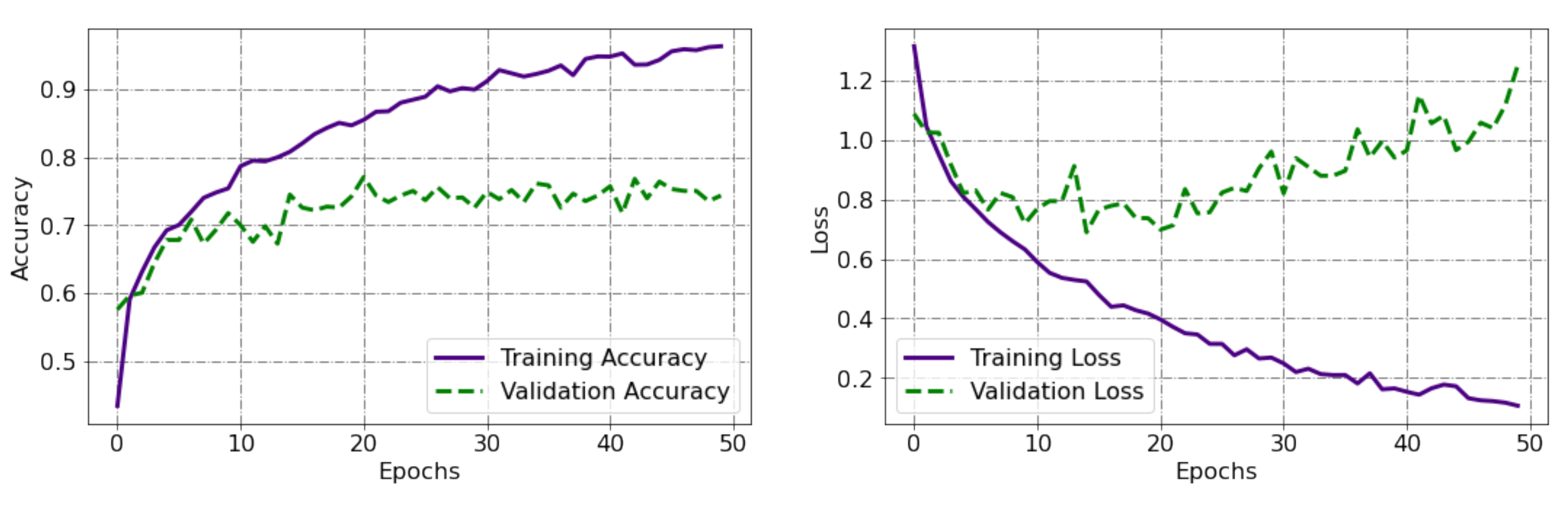
| Epoch | Mini-Batch Accuracy | Vald. Accuracy | Mini-Batch Loss | Vald. Loss |
|---|---|---|---|---|
| 1 | 37.54% | 57.22% | 1.48 | 1.10 |
| 4 | 68.53% | 67.03% | 0.82 | 0.94 |
| 8 | 74.08% | 70.44% | 0.68 | 0.74 |
| 12 | 79.09% | 72.62% | 0.55 | 0.68 |
| 16 | 82.30% | 75.20% | 0.50 | 0.69 |
| 20 | 83.55% | 73.98% | 0.41 | 0.75 |
| 24 | 88.20% | 74.52% | 0.40 | 0.77 |
| 27 | 88.09% | 74.39% | 0.32 | 0.84 |
| 31 | 91.62% | 74.39% | 0.26 | 0.78 |
| 35 | 92.04% | 76.84% | 0.23 | 0.83 |
| 39 | 93.08% | 76.29% | 0.18 | 1.06 |
| 43 | 94.56% | 72.62% | 0.16 | 1.14 |
| 47 | 93.89% | 76.98% | 0.18 | 0.90 |
| 50 | 94.48% | 76.16% | 0.15 | 1.09 |
Publisher’s Note: MDPI stays neutral with regard to jurisdictional claims in published maps and institutional affiliations. |
© 2021 by the authors. Licensee MDPI, Basel, Switzerland. This article is an open access article distributed under the terms and conditions of the Creative Commons Attribution (CC BY) license (https://creativecommons.org/licenses/by/4.0/).
Share and Cite
Endale, B.; Tullu, A.; Shi, H.; Kang, B.-S. Robust Approach to Supervised Deep Neural Network Training for Real-Time Object Classification in Cluttered Indoor Environment. Appl. Sci. 2021, 11, 7148. https://doi.org/10.3390/app11157148
Endale B, Tullu A, Shi H, Kang B-S. Robust Approach to Supervised Deep Neural Network Training for Real-Time Object Classification in Cluttered Indoor Environment. Applied Sciences. 2021; 11(15):7148. https://doi.org/10.3390/app11157148
Chicago/Turabian StyleEndale, Bedada, Abera Tullu, Hayoung Shi, and Beom-Soo Kang. 2021. "Robust Approach to Supervised Deep Neural Network Training for Real-Time Object Classification in Cluttered Indoor Environment" Applied Sciences 11, no. 15: 7148. https://doi.org/10.3390/app11157148
APA StyleEndale, B., Tullu, A., Shi, H., & Kang, B.-S. (2021). Robust Approach to Supervised Deep Neural Network Training for Real-Time Object Classification in Cluttered Indoor Environment. Applied Sciences, 11(15), 7148. https://doi.org/10.3390/app11157148