Abstract
Dimensional quality is still a major concern in additive manufacturing (AM) processes and its improvement is key to closing the gap between prototype manufacturing and industrialized production. Mass production requires the full working space of the machine to be used, although this arrangement could lead to location-related differences in part quality. The present work proposes the application of a multi-state machine performance perspective to reduce the achievable tolerance intervals of features of linear size in material extrusion (MEX) processes. Considering aspecific dimensional parameter, the dispersion and location of the distribution of measured values between different states are analyzed to determine whether the production should be treated as single-state or multi-state. A design for additive manufacturing strategy then applies global or local size compensations to modify the 3D design file and reduce deviations between manufactured values and theoretical values. The variation in the achievable tolerance range before and after the optimization of design is evaluated by establishing a target machine performance index. This strategy has been applied to an external MEX-manufactured cylindrical surface in a case study. The results show that the multi-state perspective provides a better understanding of the sources of quality variability and allows for a significant reduction in the achievable tolerance interval. The proposed strategy could help to accelerate the industrial adoption of AM process by reducing differences in quality with respect to conventional processes.
1. Introduction
In additive manufacturing (AM), a three-dimensional geometry is decomposed in bi-dimensional shapes and used to create solid parts that are built layer upon layer [1]. This basic workflow is common to different manufacturing processes, like material jetting (MJT), material extrusion (MEX), and powder bed fusion (PBF) [2]. The application of AM has evolved from prototypes to small-batches, but the objective of reaching mass production capabilities would require filling the gap between AM specification standards and the industrial needs [3]. In fact, the achievable quality is still affecting the adoption rate of AM in the consumer market [4].
Tolerance intervals (TI) are expected to be larger in AM than in traditional manufacturing processes [5], and this lack of quality has been usually addressed by adding post-processing steps [6]. Production planning in AM will require trustable information about the expected TI and the fulfillment of tolerance specifications to decide which machine or technology will be used beforehand [7].
Those works investigating dimensional quality in the AM process are frequently focused on providing a quantification of dimensional quality [8,9,10,11,12], analyzing the influence of different factors upon dimensional accuracy [13,14,15,16,17], or proposing strategies to improve dimensional quality [18,19,20,21]. Boschetto [13] modelled the dimensional deviation of parts manufactured in MEX machines as a function of the deposition angle and layer thickness. The model was verified for different materials and angles before being applied to a multi-feature case study. Huang [18] used the deviations between the manufactured surface and the target one to compensate shrinkage in a stereolithography process. Lieneke [14] used cuboids to analyze the achievable tolerances in a MEX machine, considering orientations along X, Y and Z axes. Parts were manufactured in several positions, but the results were averaged and the possible influence of position upon results was not considered. Measured dimensions were found to be dependent on orientation and nominal size, and the authors provided an estimation of the correspondent TI amplitude and location.
Minetola proposed a reference multi-feature part that was used to evaluate the dimensional accuracy of AM systems [8]. This researcher has also used the proposed test specimen to perform benchmarking comparisons between different MEX machines [8,9] and between different AM processes [12]. In these works, the deviation of each measured feature from its nominal size was divided by the tolerance factor i that corresponds to a range of basic sizes according to ISO 286-1:1988 [22]. The results were later used to determine the maximum dimensional error expected for a specific feature size range, fitting it into a particular TI. Yap [15] proposed a series of benchmark artifacts to investigate process capability and applied them to MJT. They analyzed the influence of process parameters upon dimensional quality, seeking for an optimal process configuration. Goguelin [10] used a test artifact derived from the one proposed by NIST [23] to evaluate the capabilities of a MEX equipment as part of their effort to develop a smart manufacturability assistant. Leirmo [17] proposed a test artifact and an experimental strategy to evaluate dimensional and geometrical quality in PBF. This works paid attention to the differences in dimensional quality related to position and orientation of the part within the working space, but also to the variation related to consecutively manufactured trays. Their conclusions pointed to a negligible variation of measurements between builds, whereas a clear influence of the x-y position upon part dimensions was observed.
Benchmarking artefacts frequently use a multi-feature approach to provide a global perspective of the achievable quality in terms of machine or process comparison. Nevertheless, it is difficult for a designer to anticipate the achievable tolerance for a particular feature or dimension based on benchmarking results, especially due to the variability related to process configuration, and to part location and orientation. Moreover, there are also cases where the quality indicators are not relevant from an industrial point of view [24,25]. Consequently, designers still lack clear and trustable guidance regarding which would be the achievable TI for a particular geometry to be manufactured in a particular AM machine under certain processing conditions [12].
Quality assessment in medium-to-large batches has been addressed in industrial practice by means of machine performance, process performance, and process capability analysis. These types of analyses can be conducted under the guidance of the ISO 22514 series. According to ISO 22514-1 [26], the purpose of a process is to “manufacture a product which satisfies a set of preset specifications”. Specifications can be defined for different characteristics of a product but, regarding performance or capability analysis, each characteristic must be considered independently. The analysis of machine performance or process capability has been applied to conventional processes like milling [27,28,29], turning [30], moulding [31] or welding [29].
Regarding AM processes, few works have applied the performance/capability approach to evaluate the quality of parts. Nevertheless, in recent years, several attempts to apply this type of analysis have been published. Singh [32] investigated process capability in a MJT machine for different dimensional features corresponding to a single part, although the number of replicates in this analysis (16) was too low under the accepted conventions. Preißler [33] conducted an attempt to perform a capability analysis for a MEX multi-feature specimen, but the experimental design was conducted with 25 replicas. This sample size was insufficient for a process capability study and even below the minimum of 30 replicas recommended for a machine performance analysis [34]. No information was provided regarding the manufacturing sequence and the number of parts per tray. Günay [35] conducted a capability analysis of MEX manufactured dog-bone test specimens. The significance of different process parameters upon quality was firstly analyzed. Thirty units were manufactured following a one part-per-tray sequence after determining the optimal configuration. A five-zones [36] capability categorization (from “Inadequate” to “Super”) was applied, considering the process capable for values of Cp and Cpk above 1.00. This condition led to consider the process capable to achieve an IT10 for the length and the height of the test specimen, although the quality worsened to IT11 for the width of the specimen. Siraj [37] also used a dog-bone test specimen to evaluate process capability in a low-cost MEX machine. Their results showed that the process was not in control, with an evident bias between measured sizes and target ones. Despite the fact that the specified tolerances were very large (1 mm and 2 mm ranges), the equipment was found to be not capable. Udroiu [38] conducted a machine and process capability analysis for Material Jetting (MJT) manufactured cylinders. Control charts were used to evaluate if the process was in control before calculating capability indexes. This work established a ±0.1 mm TI to evaluate machine capability and a batch size of 50 units was manufactured simultaneously in a single tray. Measured values of the diameters followed a normal distribution and, comparing the result of the capability index with the capability target index (1.67), the machine was found to be capable of achieving the expected requirements for the diameter feature. Process capability was also evaluated using three trays (50 units each) and the process was also found to be capable. Zongo [39] conducted a process capability analysis of tooling components manufactured in a laser power bed fusion (PBF) machine. This work considered the possible correlation between the position of the part in the chamber and the measured profile deviations. Although local differences were observed, they followed different patterns for consecutive trays, and capability analysis was conducted considering all manufactured parts from three different trays as a single batch.
Despite the experimental effort, machine performance or process capability studies still have to address some relevant circumstances. First, depending on the size of the part, the batch size and the available workspace, several parts could be manufactured within the same tray. This leads to the dilemma of considering AM processes as single-state [40,41] or multi-state processes [40]. Nevertheless, this possibility has not been previously considered in the available literature, where parts have been manufactured under a “single state” assumption [32,38] or under a one part-per-tray strategy [35]. Second, machine performance studies should be based on uninterrupted runs under normal operating conditions, which is a demanding condition in AM, where processes have frequently very slow cycle times, raw materials are provided in small volumes, and unavoidable critical operations (like warm-up or tray levelling) could violate repeatability conditions. Third, once the optimal process configuration has been employed in a performance analysis, there are limited possibilities of improving the results by means of a modification of such configuration.
Taking these circumstances into account, the present work proposes the application of a multi-state machine performance perspective to reduce the achievable tolerance intervals of features of linear size in material extrusion (MEX) processes. The main steps of the proposed quality improvement methodology (Figure 1) are:
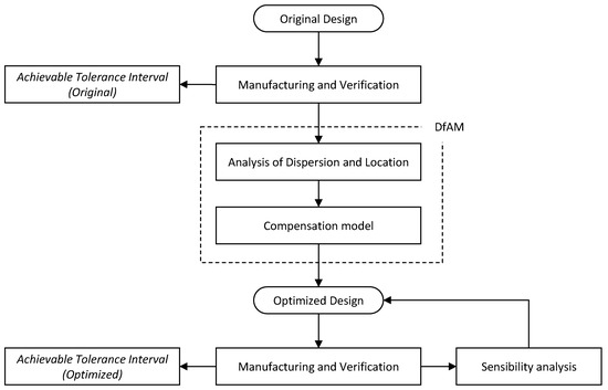
Figure 1.
Basic steps of the proposed quality improvement methodology.
- Statistical methods are used to analyse the dispersion and the location of the distribution of measured values between different states, to determine whether the production of a given geometrical feature should be treated as single-state or multi-state.
- The results are used to determine the type of compensation that should be applied by means of a design for additive manufacturing strategy.
- The 3D design files are modified to reduce deviations between manufactured values and theoretical values.
- The variation in the achievable tolerance range, before and after the optimization of design, is evaluated by establishing a target machine performance index.
The method proposed in this work is encompassed in the “design optimization” stage of the optimization framework described in [42]. More specifically, it could be applied as a previous step to a process capability analysis and serve as a guide for adjusting production to minimize the effect of machine-related inaccuracies. The objective of the proposed method is to reduce the achievable tolerance intervals in AM processes to make them a viable alternative to conventional processes. A feature of linear size (FoLS) [43] consisting of the external surface of a hollow right circular cylinder, manufactured in a MEX machine was selected as a case study.
2. Materials and Methods
2.1. Machine Performance Studies
Machine performance studies are short-term analyses, typically, used to detect and evaluate the influence of the machine on the manufacturing process without including other possible influences related to the operator, the processing conditions, the material, or the environment. The term “machine performance” is used instead of “machine capability” in accordance with ISO 22514-3 [34] because this type of analysis does not require the product characteristic to be in control. The main objectives of a performance study are to identify the probability distribution of a product characteristic, to estimate the corresponding distribution parameters, and to determine if the results are acceptable according to a quality specification. The specification for a dimensional characteristic is defined by means of an upper specification limit (U), corresponding to the highest acceptable value and a lower specification limit (L), corresponding to the lowest acceptable value. Accordingly, the TI is the range between U and L, whereas the target value (T) is the preferred or reference value for the characteristic. In a machine performance study, a series of parts are manufactured and measured. Each characteristic (X) is considered independently at a time, and the measured values for every i part (Xi) are used to determine the distribution model that better fits the results of the product characteristic. Once the statistical distribution has been determined, a reference interval is chosen for the expected result’s characteristic, following the common industrial convention of having a 99.73% of the measures within limits [41]. This interval corresponds to a to a ±3σ range for a normal distribution of values, with mean µ (X50%) and standard deviation σ. Such range would be bounded by the 99.865% distribution quantile (X99.865%) and the 0.135% distribution quantile (X0.135%), that is: between µ − 3σ and µ + 3σ. The machine performance index (Pm) evaluates the ratio between the TI and the reference interval (Equation (1)).
Nevertheless, Pm does not take into account if the process is centred or not, since it only compares the width of the intervals. Accordingly, Pm provides an estimation of the maximum theoretical performance that would be obtained if the mean value for the product characteristic matches perfectly the target value. Consequently, this index is sometimes referred to as the “potential” performance index. Situations where the mean value of the obtained distribution model and the target value are significantly different can be better described through the upper (PmkU) (Equation (2)) and the lower (PmkL) (Equation (3)) machine performance indexes.
Once both indexes have been obtained, the critical (minimum) machine performance index (Pmk) can be calculated as the minimum of PmkU and PmkL.
Although this is the usual approach regarding the application of capability studies in AM processes, there are some circumstances to be considered. Firstly, in mass production, several identical parts would be manufactured in the same tray depending on the size of the part, on the batch size, and on the working volume of the machine. If the position of each part within the manufacturing tray has an influence upon the measured values of the characteristic, this could suppose a violation of the repeatability conditions. This circumstance is related in [34] as a possibility in multiple fixture set-up, multiple-cavity, or multi-stream processes. In those cases, the reference standard to be applied would be the ISO 22514-8 [40]. This standard defines a process state as a “specific configuration of the full set of intrinsic factors”, while an intrinsic factor would be an “internal condition to the production process” which has “different aspects”.
Although in AM there are no fixtures or “cavities” involved, they have certain similarities with multi-state processes, since the location of the part within the tray can be considered as an intrinsic factor and each possible location can be assimilated to a process state. Nevertheless, this approach would be highly dependent on the specific characteristics of a production run: if each possible location is considered a process state and the location of the part within the tray could be modified by the operator, the number of process states would not be established a priori but would be dependent on production decisions (like batch volume or nesting). The ISO 22514-8 [40] addresses a multi-state process by splitting it into a set of individual states, and then comparing the dispersions and locations of the results between states. This approach is conducted using a minimum of 30 samples (N) that are obtained from n samples and j states (N = j·n), being 3 the minimum number of samples accepted for this procedure [40]. Once the parts have been manufactured, an outlier analysis should be conducted to detect and process abnormal results (excluding them from the study or trying to find the cause). Then the procedure compares the width of the local intrinsic dispersions between the different states (Dij). If the widths can be considered equal to a pooled or combined variance, then the process would be uni-modal, meaning that results for each state follow the same distribution model. If they are not equal, then the process would be multi-modal, and the practitioner could identify and correct the causes of variation or assume that this result is inherent to the process. Finally, the procedure compares the locations of the local intrinsic dispersions, estimating X50% by its mean () when it is expected that the distribution is close to symmetrical. In the case of the widths of the local intrinsic dispersions being identical, the locations would be cross-compared and, if they are found to be identical the difference is considered equal to zero (Δm = 0). If this is not the case, the results of the extreme states should be integrated according to Table 1 in [40] to obtain different estimations of the performance indexes. Accordingly, a machine performance study shall only be conducted under [34] if the process has been found to be uni-modal with a zero Δm. In this situation, the process is assimilated to a single-state.
2.2. Achievable Tolerance Interval
The calculation of machine performance indexes implies that a TI was established during the design stage. Using their experience and the product requirements, designers should be capable of defining the required TI that will make a particular characteristic acceptable. In the case of AM processes, as it was discussed in Section 1, there is a lack of technical knowledge regarding what would be the proper quality specification for a particular problem. In this work, we propose using the machine performance analysis to obtain an estimation of the TI that could be achieved for a given characteristic. This estimation of the achievable tolerance interval () is obtained by setting a target value for the performance indexes (Pm and Pmk) and then calculating the minimum that will assess such performance level.
When at least 125 samples are available, 1.33 is the acceptable target for the estimated capability or performance indexes since, given the correspondent confidence intervals, it assesses that the real values of the indexes would lie between 1.08 and 1.58 with a 99.73% probability. Nevertheless, when machine performance studies are conducted with smaller sample sizes, the target must be increased to compensate the reduction on the reliability associated to larger confidence intervals [41]. The performance and capability indexes depend on the standard deviation of the statistical distribution model, and its variation can be described by a χ2 distribution [41]. Accordingly, for small sample sizes, the χ2 distribution can be used to calculate the confidence intervals for the performance index estimation and the target value shall be increased in accordance with [41]. In the case of 50 samples or more, the adequate target value for performance indexes shall be 1.67 [38,41], and the potential shall be calculated as in Equation (4).
This calculation shall be adapted to the alternative formulations of the performance indexes described in Section 2.1 and discussed in ISO 22514-3 [34] and ISO 22514-8 [40].
2.3. DfAM Compensation Strategy
Machine performance is a powerful tool that can be used to improve the achievable quality of a product characteristic. Once the distribution model or the local intrinsic dispersion indicators (widths and locations) have been obtained, the designer has a valuable information that can be used to enhance the results. Although the optimization of the process is frequently achieved through a modification of its configuration, we propose that the retrieved information shall be used in a compensation procedure to modify the description of the design contained in the CAD file according to the procedure in Figure 2.
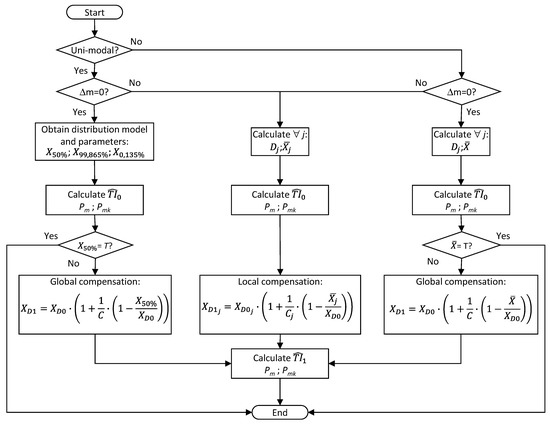
Figure 2.
Flowchart of the proposed DfAM compensation strategy considering j possible states.
The optimization of the CAD file is achieved through the modification of the dimensional parameter used for defining the studied characteristic, to compensate the expected deviation between the results and the target. This compensation will be different depending on the findings of the machine performance analysis. If the process is found to be uni-modal and the difference between locations of the intrinsic dispersions is zero, then the deviation between X50% and the reference or target T (usually coincident with the original design size XD0) will be used to calculate an optimized design size (XD1) according to Equation (5).
being C a sensibility coefficient included to model possible non-proportionalities between the changes introduced in the design file and the changes in the results.
Similarly, when the process is multi-modal but the differences of locations between the intrinsic dispersions is zero, then the deviation between and T shall be used to calculate an optimized design size (XD1) according to Equation (6).
Finally, if the process presents significant differences between the locations of the intrinsic dispersions, the DfAM proposes the application of individual compensations for each process state (j). In this case, Equation (7) would be applied to calculate each optimized size.
Accordingly, if this is the case, the parts in the tray would no longer be replicates of the same common design file, but a series of different designs tailored for each state to compensate expected deviations between results and target values.
Initially, no information would be available regarding the value of the sensibility coefficient and the practitioner should manufacture a series of parts neglecting its effect (C = 1). Once a new set of parts have been manufactured and measured, an estimation of C can be calculated as the ratio between the variation between parts manufactured under both original and optimized designs (output) and the variation of the size used in these designs (input). In the case of significant differences between the locations of the intrinsic dispersions, the sensibility coefficients can be different for each state (Cj), and they shall be calculated according to Equation (8).
2.4. Experimental Procedure: Case Study
A case study was conducted to exemplify the proposed compensation strategy. A feature of linear size (FoLS) [43] consisting of the external surface of a hollow right circular cylinder, with a target diameter of 40 mm. The part was designed in a parametric CAD software, considering a 30 mm internal diameter and a 40 mm part height. Test specimens were manufactured in a BCN3D SIGMA material extrusion equipment. This machine uses removable borosilicate glass trays with a 297 mm × 210 mm area. A polylactic acid (PLA) was selected as the model material. This material was preferred in this case study to other thermoplastics like ABS or PA because of its lower health risk, given that the equipment has an open workspace and no particle filters. The configuration parameters used in this study are provided in Table 1.

Table 1.
Processing configuration.
The layer thickness was selected after Günay [35], whereas the 25% infill is a frequently used value [44,45,46]. Deposition speed and print temperatures have been adapted after the recommendations of the Ultimaker and the actual performance of the BCN3D. This process configuration delivered a stable operation through all the tests. Following the requirements of the machine performance analysis, this configuration was not modified in any way during the manufacturing operations reflected in the present work. The parts were orientated with the cylinder axis parallel to the Z coordinate of the cartesian reference system to avoid the use of support structures and prevent the increase of the volumetric error associated to slight deviations from the vertical [47]. Part location within the tray was considered as a possible intrinsic factor that should to be analyzed under a multi-state perspective. Since an undetermined number of possible locations could be defined for the test part, it was decided that the machine performance would consider thirteen possible states (j = 13), arranged according to Figure 3. The cartesian reference system used for part placement -according to the definition in ISO/ASTM 52921:2013 [48] with the origin in the geometrical center of the tray.
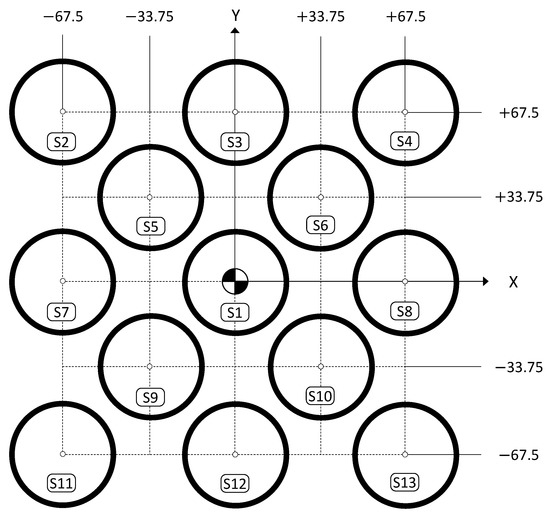
Figure 3.
Distribution of parts according to the selected thirteen states in the manufacturing tray.
The experimental procedure was divided in four steps. First, was calculated under a multi-state perspective, considering four samples (n = 4) per state and a total 52 samples (N = 52). Each sample was obtained from a different tray. Second, was directly calculated under the single-state perspective to illustrate the differences between both approaches using the same parts (52). Third, two additional trays, with 13 parts each, were manufactured to calculate the Cj and the design was optimized following the procedure in Figure 2. Fourth, an optimized set of 52 parts was manufactured and the resultant was finally calculated.
All the parts manufactured in this work were verified in a DEA Global Image 09-15-08 Coordinate Measurement Machine (CMM), calibrated according to ISO 10360-2:2009 [49]. The maximum permissible error of length measurement (E0,MPE) was (Equation (9)):
while the maximum permissible limit of the repeatability range (R0,MPL) was 2.2 µm.
The roundness profile verification strategy was defined following the methodology proposed in [50]: the relevant frequential components of geometrical deviations were calculated by means of the fast Fourier transform and the Nyquist criterion was used to determine the optimal scanning density for a reliable characterization of part geometry. As a result, nine cross-sections were digitized 4 mm apart from each other, whereas 18 points (one every 20°) were registered for each cross-section. Each part was measured thrice and the average result of those three measured was thereafter employed. Metrological operations were conducted using the PC-DMIS metrology software and the temperature in the laboratory was maintained within a range of 20 ± 2 °C. After each tray was manufactured, parts were carried to the metrology laboratory and left there for at least six hours to allow the temperature of the parts to equate with the room temperature. Statistical analysis was performed using Minitab®, whereas Solid Edge® was used for CAD design.
3. Results
Test specimens were manufactured and verified (Figure 4) according to the experimental planning.
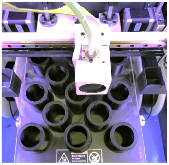
Figure 4.
Manufacturing of a tray in the BCN3D SIGMA equipment.
No special circumstances that could compromise the conditions of this study were registered. The measured values of the diameters corresponding to the four initial trays are provided in Table 2.
Table 2.
Four initial trays: measured values and calculated parameters (in mm).
3.1. Calculation of under the Multi-State Perspective
As it was mentioned in Section 2, thirteen states were considered in the multi-state perspective, and four samples were manufactured for each state. First, the Grubb’s test was performed to assure that no outlier was present at the 0.5% level of significance. Following the recommendation of [40] for the case of dimensional characteristics, it was assumed that the values follow a normal distribution. The Bartlett’s test was then performed to check the hypothesis of homogeneity between states (Figure 5a) and a 0.510 p-value was obtained. This result indicated that the null hypothesis cannot be rejected, and it was therefore accepted that the widths of the local intrinsic dispersions can be treated as identical.
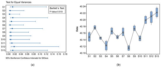
Figure 5.
Comparison between states: (a) Results of the Bartlett’s test, including the Bonferroni confidence intervals; (b) Boxplot for different states.
Assuming equal variances, the Fisher’s method was applied to cross-compare the locations of local intrinsic dispersions and determine if they could be considered identical. Thirteen states taken two at a time generated 78 possible combinations. The results of the Fisher’s test showed that 61 of those comparisons provided a p-value lower than the α-level (0.05), which implied that the null hypothesis shall be rejected, and the locations of the intrinsic intervals were significantly different for those combinations. The remaining 17 comparisons conversely, provided p-values higher than the α-level, which means that the locations can be considered equal for those pairs of states involved. Table 3 reflects exclusively the results for those pairs of states whose locations were considered to be equal.
Table 3.
Results of the Fisher individual test for difference of means between states 1.
Despite few states having equal locations according to the F-test, the overall result was that the production of the test part followed a Type 1 global intrinsic production dispersion according to ISO 22514-8 [40], since the widths of local intrinsic dispersions were equal, but the estimation of the differences in location of local intrinsic dispersions was not null. In this situation, the calculation of the shall be done according to Equation (10).
where is the half-width of the bottom-slope side of the local intrinsic dispersion, the top-slope side, and Δm the difference between the higher and the lower locations of the local intrinsic dispersion (Equation (11)).
The extreme locations of the local intrinsic dispersions were obtained for S9 ( = 40.115 mm) and S13 ( = 40.222 mm), accordingly, . The pooled standard deviation (0.0108 mm) was used to calculate the width of the local intrinsic dispersion and . Consequently, under the multiple states perspective, an achievable 0.218 mm tolerance interval was estimated.
On the other hand, when the critical performance index was applied, the was calculated considering Lm and Um. The minimum upper limit was calculated as:
which brings a result of .
Similarly, the minimum lower limit was:
which brought a result of . Assuming a centered tolerance interval of 0.552 mm was obtained. This meant that the specification required to achieve a of 1.67 should be 40 ± 0.276 mm (Figure 6b).
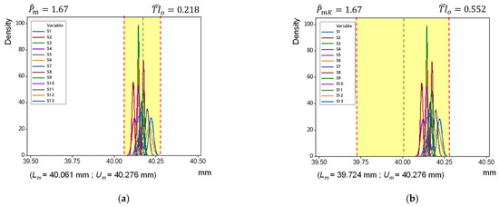
Figure 6.
Representation of and the individual distributions per state calculated under the multi-state perspective: upon the original design: (a) Calculated to assess the target performance index; (b) Calculated to assess the target critical performance index.
3.2. Calculation of under the Single-State Perspective
An alternative calculation of was performed considering the single-state hypothesis. This approach would require the parts to be manufactured in an uninterrupted run under normal operating conditions and repeatability conditions [34]. The usual recommendation is that the study should be conducted with no less than 30 specimens, maintaining constant all factors others than the machine, like the operator or the batch of material, while avoiding intermediate operations like warm-up times. These conditions are specially challenging in MEX processes for several reasons: first, these processes have usually a very slow cycle time; second, raw material is provided in small-volume coils (typically ranging from 0.5 kg to 3 kg), which makes it difficult to manufacture series of big parts from the same coil; third, the manufacturing tray is often extracted from the machine to remove the parts, and this could lead to carry out operations (warm-up, tray levelling) that could cause a disturbance on repeatability conditions. To deal with this difficulty, results from different trays were analysed to evaluate if parts could be treated as if they were a sample of a single population. Consequently, the hypothesis of homogeneity of the variances and the means were sequentially verified.
The hypothesis of homogeneity of variances was tested in first place using the Bartlett’s test. The calculated p-value was 0.983, much greater than the significance value of 0.05, which indicates that the variances can be considered equal (Figure 7a).
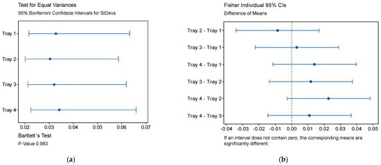
Figure 7.
Comparison between trays: (a) Results of the Bartlett’s test, including the Bonferroni confidence intervals; (b) Confidence intervals for the difference of means according to Fisher.
Then, the Fisher’s method was applied to evaluate whether pairs of means were different between consecutive trays (Figure 7b). The calculated p-values were found to be higher than the 0.05 level of significance for each pair of trays within the comparison [Table 4]. Figure 7b shows that the calculated intervals overlapped, containing the zero, which indicates that there is no statistical evidence for the means to be significantly different. It was concluded that the trays have no statistically significant effect upon the means of the measured sizes. The combination of this result with the equality of variances allows for the conclusion that the different trays can be considered as part of a single population and, consequently, the application of the ISO 22514-3 [34] did not violate the repeatability hypothesis.
Table 4.
Results of the Fisher individual test for difference of means between trays.
Given this result, the production was onwards assumed to come from a single batch, and the machine performance analysis continued with the identification of the actual distribution. An Anderson-Darling normality test was used to determine if the distribution of values was normal or not. This test compares the empirical cumulative distribution function of the measured data with the expected results of a normal distributed data. The p-value was 0.271, higher than the α-level (0.1), which indicates that the hypothesis of the data following a normal distribution cannot be rejected (Figure 8). The mean value was and the standard deviation was .
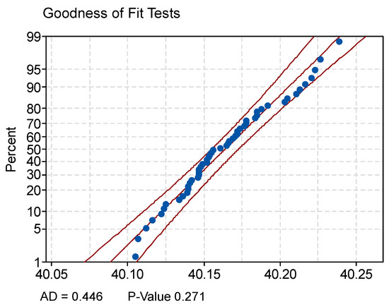
Figure 8.
Results of the Anderson-Darling normality test.
In this situation, the calculation of the shall be done according to Equation (4). Consequently, under the single-state perspective, a 0.326 mm was obtained (Figure 9a). Considering the minimum performance index (), was then calculated from the results derived from the upper () and lower () machine performance indexes. The minimum upper limit was calculated as:
whereas the minimum lower limit was:
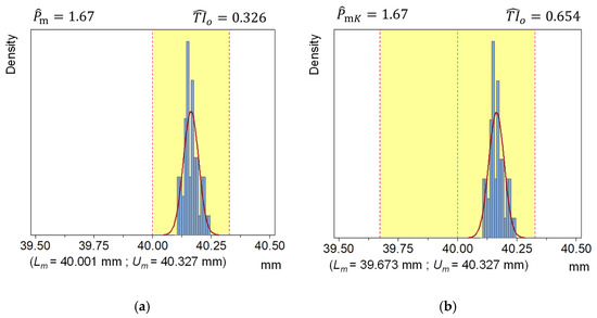
Figure 9.
Representation of and the individual distributions per state calculated under the single-state perspective upon parts manufactured with the original design: (a) Calculated to assess the target performance index; (b) Calculated to assess the target critical performance index.
Assuming a centered tolerance interval, was 0.654. This means that the specification required to achieve a of 1.67 should be 40 ± 0.327 mm (Figure 9b).
The proposed DfAM strategy was applied to individually compensate the size of each external cylindric surface regarding its relative position within the manufacturing tray. Initial compensation values for each state were calculated according to Equation (7), where the sensibility coefficients were assumed to be equal to 1. Then, two additional trays (tray 5 and tray 6) were manufactured to recalculate the sensibility coefficient for each state Cj (Equation (8)). Finally, the final values for the optimized design diameters () were also calculated. Results are provided in Table 5.
Table 5.
Calculation of the sensibility coefficients (Cj) and the optimized diameters () for each state (in mm).
3.3. Calculation of under the Multi-State Perspective
Based on the values calculated in Section 3.3, each part was redesigned, and a new set of trays (trays 7 to 10) were manufactured to evaluate the achieved improvement. Results obtained from those trays are provided in Table 6.
Table 6.
Four optimized trays: measured values and calculated parameters (in mm).
The Grubb’s test was performed to assure that no outlier was present at the 0.5% level of significance, showing that values for S12 were outliers in every manufactured tray. Accordingly, S12 was excluded from the analysis. This decision reduced the number of samples to 48 instead of 52, forcing a slight modification in the performance target that was set to 1.68 following [41]. Assuming that the values for a dimensional characteristic followed a normal distribution [40], the Bartlett’s test was performed to check the hypothesis of homogeneity between states (Figure 10a), and a 0.628 p-value was obtained. Accordingly, that the widths of the local intrinsic dispersions would be considered identical.
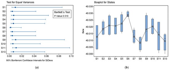
Figure 10.
Comparison between states for the optimized designs: (a) Results of the Bartlett’s test, including the Bonferroni confidence intervals; (b) Boxplot for different states.
Then, the Fisher’s method was applied to cross-compare the locations of local intrinsic dispersions and determine if they could also be considered identical. Twelve states taken two at a time generated 66 combinations and only 15 of those comparisons provided a p-value lower than the α-level (0.05), showing that the locations of the intrinsic intervals were significantly different for those combinations (Figure 10b). This result implied that the optimized diameters followed a Type 1 global intrinsic production dispersion [40]; the widths of local intrinsic dispersions were equal, but the estimation of the differences in location of local intrinsic dispersions was not null. Consequently, the calculation of the shall be done according to Equation (10). The extreme locations of the local intrinsic dispersions were obtained for S6 ( = 40.029 mm) and S8 ( = 40.008 mm), and a was obtained. The pooled standard deviation (0.0072 mm) was used to calculate the width of the local intrinsic dispersion . Finally, under the multiple states perspective, an achievable 0.093 mm tolerance interval was estimated (Figure 11a).
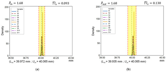
Figure 11.
Representation of and the individual distributions per state calculated under the multi-state perspective upon the optimized designs: (a) Calculated to assess the target performance index; (b) Calculated to assess the target critical performance index.
When the critical performance index was applied to the calculation of , the minimum upper limit was 40.065, and the minimum lower limit was 39.972. Assuming a centered tolerance interval, a was obtained. This means that the specification required to achieve a of 1.68 should be 40 ± 0.065 mm (Figure 11b).
4. Discussion
The proposed DfAM strategy allowed for a significant improvement in dimensional quality, according to the results, was provided in Section 3. The minimum achievable tolerance interval required to fulfil the critical machine performance target was reduced from to . Considering the standard tolerance intervals [43], the application of the proposed DfAM has resulted in a reduction of the achievable tolerance interval from IT14 to IT 11 [43]. Even if the machine performance index is considered instead of the critical one and, consequently, the deviation between the mean value and the target specification is neglected, the achievable tolerance interval is equally reduced from to . Accordingly, considering the “potential” performance, the achievable tolerance interval would be reduced from IT12 to IT 10.
These results were obtained imposing an objective of 99.73% of the manufactured parts lying within specifications, and a minimum ratio of 1.67 between tolerance interval and results dispersion. Both results demonstrate that the proposed strategy can reduce the average deviation with respect to the target value while simultaneously narrowing down the associated dispersion.
The multi-state approach employed for machine performance calculation was key to this achievement since it has allowed to understand and address the relationship between the relative position of part within the tray and the expected quality results. Conversely, although the single-state strategy could be applied without violating repeatability conditions, as it was confirmed by the Barlett’s test, the F-test and the test for normality, this approach would lead to a misinterpretation of the causes behind the quality issues. In fact, this interpretation resulted on broader achievable tolerance intervals: from the perspective of machine performance, and from the perspective of the critical machine performance. The observed differences between both strategies are mainly related to the different ways of adjusting the results to the dispersion models. In the proposed cases study, extreme values were not stochastic in a rigorous sense but related to certain locations within the manufacturing tray. Nevertheless, when they were adjusted to a normal distribution under the single-state approach, they contributed to artificially enlarging the dispersion and, consequently, affecting the calculation of the standard deviation, worsening the estimation of the achievable tolerances. Conversely, under the multi-state approach, each location presented a relatively small associated dispersion. The achievable tolerance interval was affected by this dispersion as well as by the difference between extreme states locations (mean values), but the combined effect was still lower than that derived from a single-state perspective.
The consequences of the observed differences between both approaches have a relevant influence upon the DfAM strategy. Under the single-state approach, the samples were adjusted to a normal distribution model, with a mean value of 40.164 mm and the standard deviation of 0.0325 mm. Applying a compensation procedure to the design dimension could, in the best situation, center the results around the target (40.000 mm) but this would not have any significant effect upon the dispersion of results. Since a dimensional optimization based on the single-state approach would not affect the sources of variability, the optimized tolerance interval would not be expected to improve the value obtained with the original design and the potential machine performance index (). On the other hand, under the multi-state approach, the position of the part within the tray was identified as a significant source of variability, and the DfAM strategy used this information to individually compensate the design size. This strategy reduced the inter-location variability (Figure 12), resulting on an improvement of the achievable tolerance intervals.
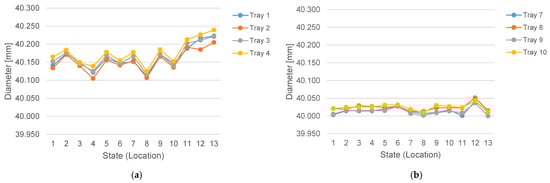
Figure 12.
Results of the multi-state DfAM strategy: (a) Original design; (b) Optimized designs.
The question of part location is not frequent in studies employing benchmarking artifacts [10,12,51] because their objectives have more to do with comparison between different processes or machines or with the analysis of the influence of process parameters than with a general assessment of their capabilities. The use of the term “capability” in some works [10] could lead to misunderstandings if the results obtained with a benchmark artifact are erroneously considered as a reference for the expected quality of a new production. In fact, the ISO 22514-1 [26] establishes that capability or performance analysis should be conducted for each characteristic individually, as the non-fulfilment of a single specification could make the whole part to be rejected. Quality prediction would require of complex modelling because AM is subjected to multiple sources of variability. Conversely, running a performance or capability study is an adequate strategy to analyze and fix quality issues for medium-to-large production batches.
The rejection of S12 in the optimized trays was determined after checking its behavior as an outlier. The reasons for this anomalous behavior were found in the values of trays 5 and 6 that were used to calculate Cj. Regarding S12, the difference between results in tray 5 and tray 6 (Table 5) were the highest among all measured values (0.026 mm). This was also the case of the differences observed for S12 within the four original trays (Table 2), which indicates that this specific location (0; −67.5) was subjected to a higher variability. Even when the Bartlett’s test did not consider this variability to be significantly different than the rest, this result could indicate that the compensation for S12 would require of more replicates to improve its accuracy. In any case, the multi-state approach allowed for the identification of such abnormal behavior and the adoption of further decisions on production arrangement.
The use of a sensibility coefficient C was necessary to properly compensate the observed deviations. The first set of compensated trays (Table 4) showed a significant reduction in the deviation between the absolute mean value of the manufactured set and the target one (from 0.164 mm to 0.040 mm), but this value was improved after the calculation of the Cj and the manufacturing of the optimized trays (0.019 mm). It was observed that the relationship between the variation applied to the design diameter (input) and the measured variation of the manufactured diameters (output) was neither directly proportional nor independent from the state (location) of the part. This conclusion is also relevant for future works, since those DfAM strategies, based on modelling size deviations and applying a compensation to the CAD file, should also consider the possibility of the response being position-dependent. Moreover, although the result was very close to the target value, there was still room for further improvement. Even after recalculating the sensitivity coefficients, results obtained from optimization did not exactly match the target values. This fact points out that the calculation of those coefficients could be even more complex than expected. Considering the results, the obtained values pointed towards a non-linear behavior, which is also a question of interest for further research.
As it was discussed before, capability analyses are hardly comparable between different geometries, processes, or configurations [35,38,39]. Nevertheless, once the production parameters have been set, attention should be drawn to those factors related to production decisions, with a special focus on the arrangement of parts within the manufacturing tray. Observations led to the conclusion that a multi-state perspective should be mandatory when analyzing machine performance in MEX AM processes. Moreover, since previous research studies have pointed out the relevance of the part position with respect to the reference axes in multiple AM processes [17,39], this finding should encourage other practitioners to adopt the multi-state perspective when working with those processes.
The proposed strategy could be applied in most industrial manufacturing facilities with a minimum adaptation effort. Nevertheless, it has to be noted that AM is not currently widespread in industry, but frequently restricted to companies that are specialized in AM. Those companies could lack the appropriate metrological equipment to conduct an optimization effort like the one described in this research. Additionally, certain technical skills regarding statistical and quality control analysis are also required, which could work as an obstacle for the adoption of the proposed strategy in small companies. Nevertheless, this should not be the case of well-stablished industrial manufacturers, accustomed to deal with quality issues, that incorporate AM to their manufacturing resources. Similarly, although the proposed strategy has been focused on MEX technologies, it could be adapted in the future to other AM processes, like PBF or MJT.
Additional future research will explore the possibilities of including process capability indexes as part of the quality improvement efforts. Since the method proposed in the present paper would allow for the approval of serial production under optimized quality conditions, long-term studies regarding process capability should be incorporated to achieve a continuous improvement of the achievable quality. The optimization effort could evolve into a progressive/iterative strategy, where each new set of parts provides an information that is incorporated to the previous results to keep the optimization parameters continuously updated. Another approach that should be explored in the future has to deal with the extension of the proposed method to a general model, encompassing a broad range of part dimensions. This multi-size approach would allow for the optimization of part dimensions even when a specific size has not been previously tested. Finally, an adaptation of this methodology to the case of geometrical tolerances is currently under development.
5. Conclusions
The present work proposes a method for improving the achievable tolerance interval of dimensional features using a multi-state machine performance analysis to feed a design for additive manufacturing strategy. Although the single-state perspective has been commonly used in AM processes, part position within the manufacturing tray is a factor that could significantly affect part quality and this influence should not be neglected. The main conclusions are:
- Machine performance analysis in AM processes shall be conducted under the multi-state perspective when multiple replicates of a part are going to be manufactured simultaneously in the same tray. This approach is necessary to evaluate if the variability of the deviations of size for a given characteristic is related to the relative position of each replicate within the tray.
- Once the analysis has determined whether the widths and locations of local intrinsic dispersions can be considered homogenous or not, the calculation of the achievable tolerance intervals shall be based on a target value for the performance indexes ( and ). The reference value (1.67) shall be used when at least 50 samples are considered, but this value shall be increased for smaller sample sizes.
- Although the optimization of the process is frequently achieved by means of a modification of its configuration, we propose a DfAM compensation procedure that uses the information retrieved from the performance analysis to modify the definition of the design contained in the CAD model. If the measured characteristic shows significant differences regarding the locations of local intrinsic dispersions, this information can be used to particularize the compensation of replicates for the different states (positions) defined. This strategy allows for a reduction of the dispersion of sizes for parts manufactured in the same tray, and for a reduction of the deviation between the mean size of the manufactured characteristic and its target value.
- The application of this methodology to a case study allowed to reduce the achievable tolerance interval from an IT14 to an IT 11 in the case of external cylindrical surfaces with a nominal size of 40 mm and manufactured in a material extrusion machine.
Results show that the multi-state approach allows for a better understanding of the sources of variation that is crucial to reduce the achievable tolerances. The proposed strategy could help to accelerate industrial adoption of AM processes, especially in those companies with a solid background in precision manufacturing and quality control that incorporate AM machines to enlarge their range of manufacturing capacities. Future research efforts should explore the possible non-linear behavior of the compensation, the extension of the methodology to other AM processes, the possibility of progressive optimization strategies based on the analysis of process capability, and the adaptation of the compensation strategy to geometrical tolerances.
Author Contributions
Conceptualization, N.B.; methodology, N.B. and D.B.; investigation, N.B., B.J.Á. and Á.N.; writing—original draft preparation, N.B. and D.B.; writing—review and editing, B.J.Á. and P.F.; supervision, B.J.Á.; project administration, P.F.; funding acquisition, D.B. All authors have read and agreed to the published version of the manuscript.
Funding
This research was funded by the Asturian Institute for Economic Development (IDEPA) and ArcelorMittal as part of the RIS3 strategy, grant number SV-PA-15-RIS3-4. It has also received funding from the Spanish Ministry of Science, Innovation and Universities (Ministerio de Economía, Industria y Competitividad, Gobierno de España—DPI2017-83068-P).
Acknowledgments
The authors wish to thank Ignacio Areces from Intelmec Ingeniería S.L. for his help.
Conflicts of Interest
The authors declare no conflict of interest. The funders had no role in the design of the study; in the collection, analyses, or interpretation of data; in the writing of the manuscript, or in the decision to publish the results.
References
- ISO/ASTM 52900. Additive Manufacturing—General Principles—Terminology; ISO: Geneva, Switzerland, 2015. [Google Scholar]
- Gibson, I.; Rosen, D.; Stucker, B. Additive Manufacturing Technologies, 2nd ed.; Springer: New York, NY, USA, 2015. [Google Scholar] [CrossRef]
- Leach, R.K.; Bourell, D.; Carmignato, S.; Donmez, A.; Senin, N. Geometrical metrology for metal additive manufacturing. CIRP Ann. Manuf. Technol. 2019, 68, 677–700. [Google Scholar] [CrossRef]
- Franco, D.; Ganga, G.M.D.; de Santa-Eulalia, L.A.; Godinho Filho, M. Consolidated and inconclusive effects of additive manufacturing adoption: A systematic literature review. Comput. Ind. Eng. 2020, 148, 106713. [Google Scholar] [CrossRef]
- Kellens, K.; Baumers, M.; Gutowski, T.G.; Flanagan, W.; Lifset, R.; Duflou, J.R. Environmental dimensions of additive manufacturing: Mapping application domains and their environmental implications. J. Ind. Ecol. 2017, 21, 49–68. [Google Scholar] [CrossRef]
- Grossi, N.; Scippa, A.; Venturini, G.; Campatelli, G. Process Parameters Optimization of Thin-Wall Machining for Wire Arc Additive Manufactured Parts. Appl. Sci. 2020, 10, 7575. [Google Scholar] [CrossRef]
- Ransikarbum, K.; Pitakaso, R.; Kim, N. A decision-support model for additive manufacturing scheduling using an integrative analytic hierarchy process and multi-objective optimization. Appl. Sci. 2020, 10, 5159. [Google Scholar] [CrossRef]
- Minetola, P.; Iuliano, L.; Marchiandi, G. Benchmarking of FDM machines though part quality using IT grades. Procedia CIRP 2016, 41, 1027–1032. [Google Scholar] [CrossRef]
- Minetola, P.; Galati, M.; Iuliano, L.; Atzeni, A.; Salmi, A. The use of self-replicated parts for improving the design and the accuracy of a low-cost 3D printer. Procedia CIRP 2018, 67, 203–208. [Google Scholar] [CrossRef]
- Goguelin, S.; Colaco, J.; Dhokia, V.; Schaefer, D. Smart manufacturability analysis for digital product development. Procedia CIRP 2017, 60, 56–61. [Google Scholar] [CrossRef]
- Pilipović, A.; Baršić, G.; Katić, M.; Rujnić, M. Repeatability and Reproducibility Assessment of a PolyJet Technology Using X-ray Computed Tomography. Appl. Sci. 2020, 10, 7040. [Google Scholar] [CrossRef]
- Minetola, P.; Calignano, F.; Galati, M. Comparing geometric tolerance capabilities of additive manufacturing systems for polymers. Addit. Manuf. 2020, 32, 101103. [Google Scholar] [CrossRef]
- Boschetto, A.; Bottini, L. Accuracy prediction in fused deposition modelling. Int. J. Adv. Manuf. Technol. 2014, 73, 913–928. [Google Scholar] [CrossRef]
- Lieneke, T.; Denzer, V.; Adam, G.A.O.; Zimmer, D. Dimensional tolerances for additive manufacturing: Experimental investigation for Fused Deposition Modelling. Procedia CIRP 2016, 43, 286–291. [Google Scholar] [CrossRef]
- Yap, Y.L.; Wang, C.; Sing, S.L.; Dikshit, V.; Yeong, W.Y.; Wei, J. Material jetting additive manufacturing: An experimental study using designed metrological benchmarks. Precis. Eng. 2017, 50, 275–285. [Google Scholar] [CrossRef]
- Park, K.; Kim, G.; No, H.; Jeom, H.W.; Kremer, G.E.O. Identification of Optimal Process Parameter Settings Based on Manufacturing Performance for Fused Filament Fabrication of CFR-PEEK. Appl. Sci. 2020, 10, 4630. [Google Scholar] [CrossRef]
- Leirmo, T.L.; Semeniuta, O. Investigating the Dimensional and Geometric Accuracy of Laser-Based Powder Bed Fusion of PA2200 (PA12): Experiment Design and Execution. Appl. Sci. 2021, 11, 2031. [Google Scholar] [CrossRef]
- Huang, Q.; Zhang, J.; Sabbagnhi, A.; Dasgupta, T. Optimal offline compensation of shape shrinkage for three-dimensional printing processes. IIE Trans. 2015, 47, 431–441. [Google Scholar] [CrossRef]
- Afazov, S.; Denmark, W.; Toralles, B.L.; Holloway, A. Distortion prediction and compensation in selective laser melting. Addit. Manuf. 2017, 17, 15–22. [Google Scholar] [CrossRef]
- Wang, A.; Song, S.; Huang, Q.; Tsung, F. In-Plane Shape-Deviation Modeling and Compensation for Fused Deposition Modeling Processes. IEEE Trans. Autom. Sci. Eng. 2018, 14, 968–976. [Google Scholar] [CrossRef]
- Shen, Z.; Bao, Y.; Xiong, G. PredNet and CompNet: Prediction and High-Precision Compensation of In-Plane Shape Deformation for Additive Manufacturing. In Proceedings of the 2019 IEEE 15th International Conference on Automation Science and Engineering (CASE), Vancouver, BC, Canada, 22–26 August 2019. [Google Scholar] [CrossRef]
- ISO 286-1:1988. ISO System of Limits and Fits—Part 1: Bases of Tolerances, Deviations and Fits; ISO: Geneva, Switzerland, 1988. [Google Scholar]
- Moylan, S.; Slotwinski, J.; Cooke, A.; Jurrens, K.; Donmez, M.A. An Additive Manufacturing Test Artifact. J. Res. Natl. Inst. Stand. Technol. 2014, 119, 429–459. [Google Scholar] [CrossRef]
- Chang, D.Y.; Huang, B.H. Studies on profile error and extruding aperture for the RP parts using the fused deposition modelling process. Int. J. Adv. Manuf. Technol. 2011, 53, 1027–1037. [Google Scholar] [CrossRef]
- El-Katatny, I.; Masood, S.H.; Morsi, Y.S. Error analysis of FDM fabricated medical replicas. Rapid Prototyp. J. 2010, 16, 36–43. [Google Scholar] [CrossRef]
- ISO 22514-1:2014. Statistical Methods in Process Management—Capability and Performance—Part 1: General Principles and Concepts; ISO: Geneva, Switzerland, 2014. [Google Scholar]
- Petrò, S.; Moroni, G. Economic aspects in the inspection of multiple geometric tolerances. In Proceedings of the ASME 2012 11th Biennial Conference on Engineering Systems Design and Analysis (ESDA2012), Nantes, France, 2–4 July 2012. [Google Scholar] [CrossRef]
- Hong, W.-P. Machine capability index evaluation of machining center. J. Mech. Sci. Technol. 2013, 10, 2905–2910. [Google Scholar] [CrossRef]
- Lépine, M., Jr.; Tahan, A.S. The relationship between geometrical complexity and process capability. J. Manuf. Sci. Eng. 2016, 138, 051009. [Google Scholar] [CrossRef]
- Kahraman, F.; Esme, U.; Kulekci, M.K.; Mersin, T.; Kazancoglu, Y.; Izmir, B. Process Capability Analysis in Machining for Quality Improvement in Turning Operations. Mater. Test. 2012, 54, 120–125. [Google Scholar] [CrossRef]
- Calaon, M.; Baruffi, F.; Fantoni, G.; Cirri, I.; Santochi, M.; Hansen, H.N.; Tosello, G. Functional Analysis Validation of Micro and Conventional Injection Molding Machines Performances Based on Process Precision and Accuracy for Micro Manufacturing. Micromachines 2020, 11, 1115. [Google Scholar] [CrossRef]
- Singh, R. Process capability study of PolyJet printing for plastic components. J. Mech. Sci. Technol. 2011, 25, 1011–1015. [Google Scholar] [CrossRef]
- Preißler, M.; Rosenberger, M.; Notni, G. An Investigation for Process Capability in Additive Manufacturing. In Proceedings of the 59th Ilmenau Scientific Colloquium, Ilmenau, Germany, 11–15 September 2017. [Google Scholar]
- ISO 22514-3:2020. Statistical Methods in Process Management—Capability and Performance—Part 3: Machine Performance Studies for Measured Data on Discrete Parts; ISO: Geneva, Switzerland, 2020. [Google Scholar]
- Günay, E.E.; Velineni, A.; Park, K.; Okudan Kremer, G.U. An Investigation on Process Capability Analysis for Fused Filament Fabrication. Int. J. Precis. Eng. Manuf. 2020, 21, 759–774. [Google Scholar] [CrossRef]
- Chen, K.S.; Huang, M.L.; Li, R.K. Process capability analysis for an entire product. Int. J. Prod. Res. 2001, 39, 4077–4087. [Google Scholar] [CrossRef]
- Siraj, I.; Bharti, P.S. Process capability analysis of a 3D printing process. J. Interdiscip. Math. 2020, 23, 175–189. [Google Scholar] [CrossRef]
- Udroiu, R.; Braga, I.C. System Performance and Process Capability in Additive Manufacturing: Quality Control for Polymer Jetting. Polymers 2020, 12, 1292. [Google Scholar] [CrossRef]
- Zongo, F.; Tahan, A.; Aidibe, A.; Brailovski, V. Intra- and Inter-Repeatability of Profile Deviations of an AlSi10Mg Tooling Component Manufactured by Laser Powder Bed Fusion. J. Manuf. Mater. Process. 2018, 2, 56. [Google Scholar] [CrossRef]
- ISO 22514-8:2014. Statistical Methods in Process Management—Capability and Performance—Part 8: Machine Performance of a Multi-State Production Process; ISO: Geneva, Switzerland, 2014. [Google Scholar]
- Quality Management in the Bosch Group. Technical Statistics—Booklet No. 9—Machine and Process Capability, 11th ed.; Robert Bosch GmbH: Gerlingen, Germany, 2019. [Google Scholar]
- Beltrán, N.; Blanco, D.; Álvarez, B.J.; Noriega, A.; Fernández, P. Dimensional and geometrical quality enhancement in additively manufactured parts: Systematic framework and a case study. Materials 2019, 12, 3937. [Google Scholar] [CrossRef] [PubMed]
- ISO 286-1:2010. Geometrical Product Specifications (GPS)—ISO Code System for Tolerances on Linear Sizes—Part 1: Basis of Tolerances, Deviations and Fits; ISO: Geneva, Switzerland, 2010. [Google Scholar]
- Bartolai, J.; Wilson-Heid, A.E.; Kruse, J.R.; Beese, A.M.; Simpson, T.W. Full Field Strain Measurement of Material Extrusion Additive Manufacturing Parts with Solid and Sparse Infill Geometries. JOM 2021, 71, 871–879. [Google Scholar] [CrossRef]
- Kumar, K.S.; Soundararajan, R.; Shanthosh, G.; Saravanakumar, P.; Ratteesh, M. Augmenting effect of infill density and annealing on mechanical properties of PETG and CFPETG composites fabricated by FDM. Mater. Today Proc. 2021, 45, 2186–2191. [Google Scholar] [CrossRef]
- Sedlak, J.; Hrusecka, D.; Jurickova, E.; Hrbackova, L.; Spisak, L.; Joska, Z. Analysis of test plastic samples printed by the additive method fused filament fabrication. MM Sci. J. 2021, 1, 4283–4290. [Google Scholar] [CrossRef]
- Masood, S.H.; Rattanawong, W.; Iovenitti, P. Part Build Orientations Based on Volumetric Error in Fused Deposition Modelling. Int. J. Adv. Manuf. Technol. 2000, 16, 162–168. [Google Scholar] [CrossRef]
- ISO/ASTM 52921:2013. Standard Terminology for Additive Manufacturing—Coordinate Systems and Test Methodologies; ISO: Geneva, Switzerland, 2013. [Google Scholar]
- ISO 10360-2:2009. Geometrical Product Specifications (GPS)—Acceptance and Reverification Tests for Coordinate Measuring Machines (CMM)—Part 2: CMMs Used for Measuring Size; ISO: Geneva, Switzerland, 2009. [Google Scholar]
- Beltrán, N.; Álvarez, B.J.; Blanco, D.; Peña, F.; Fernández, P. A Design for Additive Manufacturing Strategy for Dimensional and Geometrical Quality Improvement of PolyJet-Manufactured Glossy Cylindrical Features. Polymers 2021, 13, 1132. [Google Scholar] [CrossRef] [PubMed]
- Martínes, S.; Ortega, N.; Celentano, D.; Sánchez Egea, J.A.; Ukar, E.; Lamikiz, A. Analysis of the Part Distortions for Inconel 718 SLM: A Case Study on the NIST Test Artifact. Materials 2020, 13, 5087. [Google Scholar] [CrossRef]
Publisher’s Note: MDPI stays neutral with regard to jurisdictional claims in published maps and institutional affiliations. |
© 2021 by the authors. Licensee MDPI, Basel, Switzerland. This article is an open access article distributed under the terms and conditions of the Creative Commons Attribution (CC BY) license (https://creativecommons.org/licenses/by/4.0/).