The Design and Implementation of an Inertial GNSS Odometer Integrated Navigation System Based on a Federated Kalman Filter for High-Speed Railway Track Inspection

Abstract

The detection of track geometry parameters is essential for the safety of high-speed railway operation. To improve the accuracy and efficiency of the state detector of track geometry parameters, in this study we propose an inertial GNSS odometer integrated navigation system based on the federated Kalman, and a corresponding inertial track measurement system was also developed. This paper systematically introduces the construction process for the Kalman filter and data smoothing algorithm based on forward filtering and reverse smoothing. The engineering results show that the measurement accuracy of the track geometry parameters was better than 0.2 mm, and the detection speed was about 3 km/h. Thus, compared with the traditional Kalman filter method, the proposed design improved the measurement accuracy and met the requirements for the detection of geometric parameters of high-speed railway tracks.

1. Introduction

Railway track irregularities are caused by vehicle dynamics and natural degradation. Changes in track geometric parameters directly affect the operational safety of trains and are the main factors affecting determining the speed and smoothness of the train [1,2]. The geometric parameters of a track comprise seven internal track parameters—track gauge, track direction, and high and low, horizontal (ultra-high), versine, warp, and track gauge change rate—and two external track geometry parameters—lateral and vertical deviations from the track midline to the left and right of the track relative to the design line position [3].

The Chinese railway department implements a comprehensive integrated inspection and monitoring program for railroad infrastructure according to the principle of “dynamic inspection as the main, static inspection as a supplement” [4]. The dynamic inspection vehicle carries out high-accuracy and high-efficiency dynamic inspection of internal geometric parameters of tracks for all lines [5], but its mileage positioning accuracy is low. In addition, the maintenance department use a track geometry state detector to carry out precise mileage positioning and detection of the external parameters of the track for problematic sections, which is used to guideline repair and maintenance. Furthermore, the railway maintenance department applies the track geometry state detector to periodically measure the condition of the static geometry of lines in its jurisdiction, for which the detection task is demanding. The operating length of high-speed railway in China has reached 40,000 km. The trunk line length of a single railway engineering department may be up to hundreds of kilometers, and the maintenance time used for detection of track geometric parameters is about 4 h [6,7]. Thus, the detection period is short, and the task is challenging [8,9]. Consequently, there is an urgent need for efficient and high-accuracy equipment for the measurement of track geometric parameters.

Based on the different types of track geometric parameters measured, track geometry testing equipment can be divided into absolute and relative measuring types. Absolute measurement equipment consists of track geometry condition measuring instruments, which are used to measure the track geometry parameters of lines dedicated to passengers. This equipment is composed of two parts—a total station and a detector—and has a measurement efficiency of about 160 m/h [10,11]. Various absolute measurement track detectors have passed the measurement certification of the China Railway Group Corporation and are widely used [12]. The testing parameters of this equipment are complete, yielding high testing accuracy. However, such detectors rely on the track control point (CPIII) to operate, and their testing efficiency is low.

Amberg (Switzerland), Trimble (USA), and the Railway Engineering Consulting Group Co., Ltd. developed the “two rolleys system”, which improves measurement efficiency to 1.5 km/h. However, the measurement accuracy of this system is low, and can only be used for the measurement of geometric parameters of ballast track [13]. The GRP1000 IMS of Amberg (Switzerland), which combines the total station and inertial measurement unit with the track inspection instrument in a single vehicle system, performs a CPIII resection measurement every 60 m, thus resulting in a measurement efficiency of 1.5 km/h. However, due to frequent station changes by the total station and lapping of the measured section, the working efficiency is reduced, and “lap error” can occur [14].

Harnessing the rapid development of precise positioning techniques, such as global navigation satellite systems (GNSS), and using the GNSS real-time kinematic (RTK) technique, HTA Burgdorf developed a track surveying platform in cooperation with terra vermessungen AG, Switzerland to improve the measurement efficiency for external parameters of tracks [15]. Yildiz Technical University developed a multisensor railway track geometry surveying system, which integrated the linear variable differential transformers, inclinometer, GNSS receiver, total station, and an adaptive Kalman filter model to estimate the geometric parameters of tracks [16,17].

Relative measurement track inspection equipment, also known as track checkers, which use mobile or static laser string measurement methods, can only detect the internal geometric parameters of tracks [18,19]. Combined with odometer output mileage information, the track internal geometry parameters are measured using the chord surveying method [20,21]. In addition, Xi’an Safeway developed a rail track inspection system based on a dual antenna Global Positioning System (GPS)-aided approach [22,23]. The inertial measurement method using the dual gyroscope scheme is unable to realize accurate modeling or compensate for gyroscope error, Earth rotation angular velocity, and the implied angular velocity, which results in a reduced measurement accuracy. These problems with the pure gyroscope system are partially corrected by the dual-antenna GPS-aided inertial navigation system, but the measurement accuracy of motion parameters is low.

Based on high-accuracy absolute solutions provided by RTK, Wuhan University integrated an inertial navigation system with a geodetic surveying apparatus and designed a modular system (TGMT) based on aided INS, which can be configured according to different surveying tasks. With a GNSS/INS configuration, this system offers good repeatability of measurements of track irregularities in both horizontal and vertical directions, with an error of less than 0.3 mm [24]. However, with increasing baseline length, the correlation of atmospheric errors decreases, resulting in a decrease to RTK positioning accuracy. A novel track measurement system based on GNSS/INS and multisensors was developed by Tsinghua University and obtained 2 mm accuracy for both lateral and vertical deviations of the track, and 1 mm horizontal accuracy and 1.5 mm vertical accuracy for the deformation point [25]. To obtain high-accuracy absolute coordinates, the system not only relies on a GNSS CORS station, but also needs to stand still for 5 min every 150 m, which inevitably reduces its efficiency and increases the cost. To reduce costs and improve the measuring efficiency, a multisensor fusion system consisting of multiconstellation global navigation satellite systems (GNSS)-based precise point positioning, an inertial navigation system, odometer, and track gauge was proposed by the German Research Centre for Geosciences, which was further enhanced using a Rauch–Tung–Striebel smoother. This system reached a measurement accuracy of approximately 0.25, 0.59, 0.65, and 0.48 mm for the super elevation, horizontal, vertical, and gauge components, respectively [26].

Since 2013, we have been engaged in the research and development of a high-speed railway track measurement system based on GNSS/INS multi-sensors. The system has realized high efficiency and a 0.47 mm measurement accuracy of the internal geometric parameters of tracks, but its engineering application algorithm is still based on the classical Kalman filter method [27,28,29]. The selection of the filter method and the design of the filter are highly important for the accuracy and stability of the inertial/GNSS/odometer integrated navigation system. In this study, to address the issue of poor fault tolerance performance resulting from the use of a centralized filter, and the large computational effort necessitated by the high-dimensional characteristic of the multisensor filtering system [30], a federated filter was designed to realize the advantages of an inertial/GNSS/odometer. Then, a forward–backward smoothing method was developed to apply to the federated filter results, to further improve the integrated accuracy and corresponding track measurement system. The test results show that the measurement accuracy of track geometry parameters is less than 0.2 mm, and the detection speed is about 3 km/h, which meets the requirements for high-accuracy and high-efficiency high-speed railway track state detection.

2. Basic Principles of the Integrated Navigation System for the Inertial Track Geometry State Detector

2.1. Definition of the Common Coordinate System

• Carrier coordinate system (“b system”):

As shown in Figure 1, the track geometry state detector carrier coordinate system is OX_bY_bZ_b, where the origin of O is the center point of the car body structure; the Y_b axis is along the longitudinal axis of the track geometry state detector pointing in the direction of motion; the X_b axis is along the track geometry state detector horizontal axis to the right; and the Z_b axis is vertical. The X_b, Y_b, and Z_b axes constitute the right rectangular coordinate system.

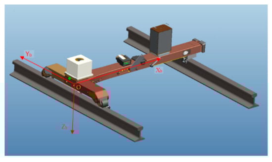
Figure 1. The carrier coordinate system (b system).

• Geographical coordinate system (“n system”):

As shown in Figure 2, the geographic coordinate system is OX_nY_nZ_n, where the origin of O is the center of the mass of the carrier; the X_n and Y_n axes are in the local horizontal plane, pointing to the east and north, respectively; and the Z_n axis points to the sky along the local vertical line. The geographic coordinate system moves with the carrier, and the coordinate axis maintains its original definite direction.

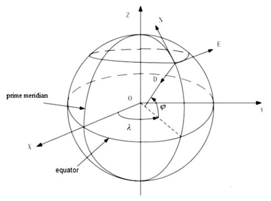
Figure 2. The geographic coordinate system (n system).

2.2. Strapdown Solution Arrangement of Inertial Navigation System

The navigation solution of the inertial navigation system adopts the north-pointing position system, and the navigation coordinate system adopts the geographic coordinate system [31]. The strapdown solution process of the inertial navigation system is shown in Figure 3.

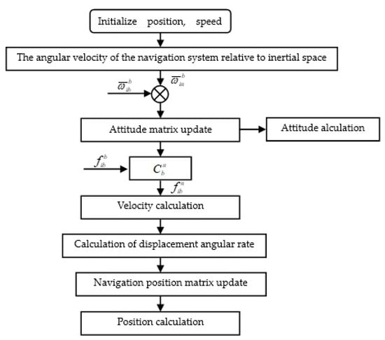
Figure 3. Strapdown solution flow of the inertial navigation system.

3. Federated Kalman Filter Design

In this paper, the federated Kalman filter was designed as the inertial/odometer dead-recursive sub-Kalman filter, the inertial/satellite integrated navigation sub-Kalman filter, and a main filter.

3.1. Error Model of Strapdown Inertial Navigation System

The error model of the strapdown inertial navigation system [30] was based on the ellipsoid model of Earth. The attitude error equation of the strapdown inertial navigation system is shown in Equation (1):

$$\{\begin{array}{c}{\dot{\mathsf{\phi } }}_{\mathrm{E}}=-\frac{{\mathsf{\delta }\mathrm{V}}_{\mathrm{N}}}{{\mathrm{R}}_{\mathrm{M}}+\mathrm{H}}{+(\mathsf{\omega }}_{\mathrm{ie}}\sin \mathrm{L}+\frac{{\mathrm{V}}_{\mathrm{E}}\tan \mathrm{L}}{{\mathrm{R}}_{\mathrm{N}}+\mathrm{H}}{)\mathsf{\phi }}_{\mathrm{N}}-{(\mathsf{\omega }}_{\mathrm{ie}}\cos \mathrm{L}+\frac{{\mathrm{V}}_{\mathrm{E}}}{{\mathrm{R}}_{\mathrm{N}}+\mathrm{H}}{)\mathsf{\phi }}_{\mathrm{U}}+\frac{{\mathrm{V}}_{\mathrm{N}}}{{{(\mathrm{R}}_{\mathrm{M}}+\mathrm{H})}^2}{\mathsf{\delta }\mathrm{H}+\mathsf{\epsilon }}_{\mathrm{E}}\\ {\dot{\mathsf{\phi } }}_{\mathrm{N}}=\frac{{\mathsf{\delta }\mathrm{V}}_{\mathrm{E}}}{{\mathrm{R}}_{\mathrm{N}}+\mathrm{H}}-{\mathsf{\omega }}_{\mathrm{ie}}{\sin \mathrm{L}\mathsf{\delta }\mathrm{L}-(\mathsf{\omega }}_{\mathrm{ie}}\sin \mathrm{L}+\frac{{\mathrm{V}}_{\mathrm{E}}\tan \mathrm{L}}{{\mathrm{R}}_{\mathrm{N}}+\mathrm{H}}{)\mathsf{\phi }}_{\mathrm{E}}-\frac{{\mathrm{V}}_{\mathrm{N}}}{{\mathrm{R}}_{\mathrm{M}}+\mathrm{H}}{\mathsf{\phi }}_{\mathrm{U}}-\frac{{\mathrm{V}}_{\mathrm{E}}}{{{(\mathrm{R}}_{\mathrm{N}}+\mathrm{H})}^2}{\mathsf{\delta }\mathrm{H}+\mathsf{\epsilon }}_{\mathrm{N}}\\ {\dot{\mathsf{\phi } }}_{\mathrm{U}}=\frac{{\tan \mathrm{L}\mathsf{\delta }\mathrm{V}}_{\mathrm{E}}}{{\mathrm{R}}_{\mathrm{N}}+\mathrm{H}}{+(\mathsf{\omega }}_{\mathrm{ie}}\cos \mathrm{L}+\frac{{\mathrm{V}}_{\mathrm{E}}{\sec }^2\mathrm{L}}{{\mathrm{R}}_{\mathrm{N}}+\mathrm{H}}{)\mathsf{\delta }\mathrm{L}+(\mathsf{\omega }}_{\mathrm{ie}}\cos \mathrm{L}+\frac{{\mathrm{V}}_{\mathrm{E}}}{{\mathrm{R}}_{\mathrm{N}}+\mathrm{H}}{)\mathsf{\phi }}_{\mathrm{E}}+\frac{{\mathrm{V}}_{\mathrm{N}}{\mathsf{\phi }}_{\mathrm{N}}}{{\mathrm{R}}_{\mathrm{M}}+\mathrm{H}}-\frac{{\mathrm{V}}_{\mathrm{E}}\tan \mathrm{L}\mathsf{\delta }\mathrm{H}}{{{(\mathrm{R}}_{\mathrm{N}}+\mathrm{H})}^2}{+\mathsf{\epsilon }}_{\mathrm{U}}\end{array}$$

(1)

where ${\mathsf{\omega }}_{\mathrm{ie}}$ is the Earth’s rotation angular velocity; E, N, and U represent the geographical east, north, and upward directions, respectively; L is latitude in the WGS84 coordinate system; H is height in the WGS84 coordinate system; ${\mathrm{V}}_{\mathrm{E}}$, ${\mathrm{V}}_{\mathrm{N}}$,${ \mathrm{V}}_{\mathrm{U}}$are the geographically eastward, northward, and astronomical components of motion velocity in the navigation coordinate system n, respectively; ${ \mathrm{R}}_{\mathrm{M}}$ is the main curvature radius of the meridian; ${\mathrm{R}}_{\mathrm{N}}$is the main curvature radius of the prime vertical; ${\mathsf{\phi }}_{\mathrm{E}}$, ${\mathsf{\phi }}_{\mathrm{N}}$, ${\mathsf{\phi }}_{\mathrm{U}}$ are the attitude angle error of the heading, pitching, and roll angles in the navigation coordinate system, respectively; ${\mathsf{\delta }\mathrm{V}}_{\mathrm{E}}$, ${\mathsf{\delta }\mathrm{V}}_{\mathrm{N}}$, ${\mathsf{\delta }\mathrm{V}}_{\mathrm{U}}$are the east, north, and upwards velocity errors in the navigation system, respectively; $\mathsf{\delta }\mathrm{L}$ is the latitude position errors in the navigation coordinate system; and ${\mathsf{\epsilon }}_{\mathrm{E}}$, ${\mathsf{\epsilon }}_{\mathrm{N}}$, ${\mathsf{\epsilon }}_{\mathrm{U}}$ are the gyro angular rate output errors in the east, north, and upward directions in the n system, respectively.

The velocity error equation of the strapdown inertial navigation system is shown in Equation (2):

$$\begin{gathered} \{\begin{array}{c}\begin{array}{c}\mathsf{\delta }{\dot{\mathsf{V}}}_{\mathsf{E}}={\mathrm{f}}_{\mathrm{N}}{\mathsf{\phi }}_{\mathrm{U}}-{\mathrm{f}}_{\mathrm{U}}{\mathsf{\phi }}_{\mathrm{N}}+(\frac{{\mathrm{V}}_{\mathrm{N}}\tan \mathrm{L}-{\mathrm{V}}_{\mathrm{U}}}{{\mathrm{R}}_{\mathrm{N}}+\mathrm{H}}{)\mathsf{\delta }\mathrm{V}}_{\mathrm{E}}{+(2\mathsf{\omega }}_{\mathrm{ie}}\sin \mathrm{L}+\frac{{\mathrm{V}}_{\mathrm{E}}\tan \mathrm{L}}{{\mathrm{R}}_{\mathrm{N}}+\mathrm{H}}{)\mathsf{\delta }\mathrm{V}}_{\mathrm{N}}{+(2\mathsf{\omega }}_{\mathrm{ie}}{\mathrm{V}}_{\mathrm{N}}\cos \mathrm{L}+\\ \frac{{\mathrm{V}}_{\mathrm{E}}{\mathrm{V}}_{\mathrm{N}}{\sec }^2\mathrm{L}}{{\mathrm{R}}_{\mathrm{N}}+\mathrm{H}}{+2\mathsf{\omega }}_{\mathrm{ie}}{\mathrm{V}}_{\mathrm{U}}{\sin \mathrm{L})\mathsf{\delta }\mathrm{L}-(2\mathsf{\omega }}_{\mathrm{ie}}\cos \mathrm{L}+\frac{{\mathrm{V}}_{\mathrm{E}}}{{\mathrm{R}}_{\mathrm{N}}+\mathrm{H}}{)\mathsf{\delta }\mathrm{V}}_{\mathrm{U}}+\frac{{\mathrm{V}}_{\mathrm{E}}{\mathrm{V}}_{\mathrm{U}}-{\mathrm{V}}_{\mathrm{E}}{\mathrm{V}}_{\mathrm{N}}\tan \mathrm{L}}{{{(\mathrm{R}}_{\mathrm{N}}+\mathrm{H})}^2}\mathsf{\delta }\mathrm{H}+{\nabla }_{\mathrm{E}}\end{array}\\ \mathsf{\delta }{\dot{\mathsf{V}}}_{\mathsf{N}}={\mathrm{f}}_{\mathrm{U}}{\mathsf{\phi }}_{\mathrm{E}}-{\mathrm{f}}_{\mathrm{E}}{\mathsf{\phi }}_{\mathrm{U}}-{2(\mathsf{\omega }}_{\mathrm{ie}}\sin \mathrm{L}+\frac{{\mathrm{V}}_{\mathrm{E}}\tan \mathrm{L}}{{\mathrm{R}}_{\mathrm{N}}+\mathrm{H}}{)\mathsf{\delta }\mathrm{V}}_{\mathrm{E}}-\frac{{\mathrm{V}}_{\mathrm{U}}{\mathsf{\delta }\mathrm{V}}_{\mathrm{N}}}{{\mathrm{R}}_{\mathrm{M}}+\mathrm{H}}-\frac{{\mathrm{V}}_{\mathrm{N}}{\mathsf{\delta }\mathrm{V}}_{\mathrm{U}}}{{\mathrm{R}}_{\mathrm{M}}+\mathrm{H}}- \\ {(2\mathsf{\omega }}_{\mathrm{ie}}\cos \mathrm{L}+\frac{{\mathrm{V}}_{\mathrm{E}}{\sec }^2\mathrm{L}}{{\mathrm{R}}_{\mathrm{N}}+\mathrm{H}}{)\mathrm{V}}_{\mathrm{E}}\mathsf{\delta }\mathrm{L}+\frac{{\mathrm{V}}_{\mathrm{N}}{\mathrm{V}}_{\mathrm{U}}{+\mathrm{V}}_{\mathrm{E}}{\mathrm{V}}_{\mathrm{E}}\tan \mathrm{L}}{{{(\mathrm{R}}_{\mathrm{N}}+\mathrm{H})}^2}\mathsf{\delta }\mathrm{H}+{\nabla }_{\mathrm{N}}\\ \begin{array}{c}\mathsf{\delta }{\dot{\mathsf{V}}}_{\mathsf{U}}={\mathrm{f}}_{\mathrm{N}}{\mathsf{\phi }}_{\mathrm{E}}{+\mathrm{f}}_{\mathrm{E}}{\mathsf{\phi }}_{\mathrm{N}}{+2(\mathsf{\omega }}_{\mathrm{ie}}\cos \mathrm{L}+\frac{{\mathrm{V}}_{\mathrm{E}}}{{\mathrm{R}}_{\mathrm{N}}+\mathrm{H}}{)\mathsf{\delta }\mathrm{V}}_{\mathrm{E}}+2\frac{{\mathrm{V}}_{\mathrm{N}}{\mathsf{\delta }\mathrm{V}}_{\mathrm{N}}}{{\mathrm{R}}_{\mathrm{M}}+\mathrm{H}}-{2\mathsf{\omega }}_{\mathrm{ie}}{\mathrm{V}}_{\mathrm{E}}\sin \mathrm{L}\mathsf{\delta }\mathrm{L}-\\ \frac{{\mathrm{V}}_{\mathrm{E}}{\mathrm{V}}_{\mathrm{E}}{+\mathrm{V}}_{\mathrm{N}}{\mathrm{V}}_{\mathrm{N}}}{{{(\mathrm{R}}_{\mathrm{N}}+\mathrm{H})}^2}\mathsf{\delta }\mathrm{H}+{\nabla }_{\mathrm{U}}\end{array}\end{array} \end{gathered}$$

(2)

where$\mathsf{\delta }\mathrm{H}$ is the height position errors in the navigation coordinate system; ${\mathrm{f}}_{\mathrm{E}}$, ${\mathrm{f}}_{\mathrm{N}}$, and ${\mathrm{f}}_{\mathrm{U}}$ are the specific force of accelerometer in the east, north, and upward directions in the n system, respectively; $\mathrm{and} {\nabla }_{\mathrm{E}}$,${\nabla }_{\mathrm{N}}$, and${\nabla }_{\mathrm{U}}$are the specific force error of accelerometer in the east, north, and upward directions in the n system, respectively.

The position error equation of the strapdown inertial navigation system is shown in Equation (3):

$$\{\begin{array}{c}\mathsf{\delta }\dot{\mathrm{L}}=\frac{{\mathsf{\delta }\mathrm{V}}_{\mathrm{N}}}{{\mathrm{R}}_{\mathrm{M}}+\mathrm{H}}-\frac{{\mathrm{V}}_{\mathrm{N}}}{{{(\mathrm{R}}_{\mathrm{M}}+\mathrm{H})}^2}\mathsf{\delta }\mathrm{H}\\ \mathsf{\delta }\dot{\lambda }=\frac{\sec \mathrm{L}}{{\mathrm{R}}_{\mathrm{N}}+\mathrm{H}}{\mathsf{\delta }\mathrm{V}}_{\mathrm{E}}+\frac{{\mathrm{V}}_{\mathrm{E}}\sec \mathrm{LtanL}}{{\mathrm{R}}_{\mathrm{N}}+\mathrm{H}}\mathsf{\delta }\mathrm{L}-\frac{{\mathrm{V}}_{\mathrm{E}}\sec \mathrm{L}}{{{(\mathrm{R}}_{\mathrm{N}}+\mathrm{H})}^2}\mathsf{\delta }\mathrm{H}\\ \mathsf{\delta }\dot{\mathrm{H}}={\mathsf{\delta }\mathrm{V}}_{\mathrm{U}}\end{array}$$

(3)

In this study, the errors of the inertial measurement unit (IMU) were calibrated before use, and it was considered that the errors of IMU after calibration and compensation were random zero bias and white noise. The random zero bias constant error equations of the gyroscope and accelerometer are shown in Equations (4) and (5), respectively:

$${\dot{\epsilon }}_{\mathrm{x}}=0, {\dot{\epsilon }}_{\mathrm{y}}=0, {\dot{\epsilon }}_{\mathrm{z}}=0$$

(4)

$${\dot{\nabla }}_{\mathrm{x}}=0,{\dot{\nabla }}_{\mathrm{y}}=0, {\dot{\nabla }}_{\mathrm{z}}=0$$

(5)

where ${\mathsf{\epsilon }}_{\mathrm{x}}$, ${\mathsf{\epsilon }}_{\mathrm{y}}$, ${\mathsf{\epsilon }}_{\mathrm{z}}$, and ${\nabla }_{\mathrm{x}}$, ${\nabla }_{\mathrm{y}}$, and ${\nabla }_{\mathrm{z}}$ are the constant zero bias of the gyroscope and the constant zero deviation of the accelerometer on the three measurement axes of the inertial measurement unit, respectively.

3.2. Inertial/Odometer Dead-Reckoning Error Model

The inertial/odometer navigation calculation algorithm primarily consisted of an attitude updating algorithm and a position updating algorithm. Using the strapdown inertial navigation system error equation, the attitude error equation and position error equation based on the inertial/odometer navigation calculation can be obtained. The main error sources of the navigation calculation are attitude, gyroscope data measurement, and odometer measurement errors.

3.2.1. Position Error Equation of Dead Reckoning

The measurement error of the odometer data was mainly due to the calibration coefficient error ${\mathsf{\delta }\mathrm{K}}_{\mathrm{D}}$. Thus, the odometer speed error equation can be obtained as follows:

$${\mathsf{\delta }\mathrm{V}}_{\mathrm{D}}^{\mathrm{n}}={\mathrm{V}}_{\mathrm{D}}^{\mathrm{n}}\times {\mathsf{\phi }}_{\mathrm{D}}+{\mathsf{\delta }\mathrm{K}}_{\mathrm{D}}{\mathrm{V}}_{\mathrm{D}}^{\mathrm{n}}$$

(6)

where ${\mathrm{V}}_{\mathrm{D}}$ is the actual running speed of the odometer and ${\mathsf{\phi }}_{\mathrm{D}}$ is the attitude angle error. The position error equation of dead reckoning is shown in Equation (7):

$$\{\begin{array}{c}\mathsf{\delta }\dot{\mathrm{L}}=\frac{{\mathsf{\delta }\mathrm{V}}_{\mathrm{N}}}{{\mathrm{R}}_{\mathrm{M}}+\mathrm{H}}-\frac{{\mathrm{V}}_{\mathrm{N}}}{{{(\mathrm{R}}_{\mathrm{M}}+\mathrm{H})}^2}\mathsf{\delta }\mathrm{H}\\ \mathsf{\delta }\dot{\mathsf{\lambda }}=\frac{\sec \mathrm{L}}{{\mathrm{R}}_{\mathrm{N}}+\mathrm{H}}{\mathsf{\delta }\mathrm{V}}_{\mathrm{E}}+\frac{{\mathrm{V}}_{\mathrm{E}}\sec \mathrm{LtanL}}{{\mathrm{R}}_{\mathrm{N}}+\mathrm{H}}\mathsf{\delta }\mathrm{L}-\frac{{\mathrm{V}}_{\mathrm{E}}\sec \mathrm{L}}{{{(\mathrm{R}}_{\mathrm{N}}+\mathrm{H})}^2}\mathsf{\delta }\mathrm{H}\\ \mathsf{\delta }\dot{\mathrm{H}}={\mathsf{\delta }\mathrm{V}}_{\mathrm{U}}\end{array}$$

(7)

where ${\mathsf{\delta }\mathrm{V}}_{\mathrm{E}}$, ${\mathsf{\delta }\mathrm{V}}_{\mathrm{N}}$, and ${\mathsf{\delta }\mathrm{V}}_{\mathrm{U}}$ are the components of the odometer speed error along the XYZ axis in the navigation coordinate system. Equation (7) was expanded to obtain Equation (8):

$$\{\begin{array}{c}\mathsf{\delta }\dot{\mathrm{L}}=\frac{{\mathrm{V}}_{\mathrm{N}}}{{\mathrm{R}}_{\mathrm{M}}+\mathrm{H}}{\mathsf{\delta }\mathrm{K}}_{\mathrm{D}}-\frac{{\mathrm{V}}_{\mathrm{E}}}{{\mathrm{R}}_{\mathrm{M}}+\mathrm{H}}{\mathsf{\phi }}_{\mathrm{U}}\\ \mathsf{\delta }\dot{\mathsf{\lambda }}=\frac{{\mathrm{V}}_{\mathrm{N}}\sec \mathrm{L}}{{\mathrm{R}}_{\mathrm{N}}+\mathrm{H}}{\mathsf{\phi }}_{\mathrm{U}}+\frac{{\mathrm{V}}_{\mathrm{E}}\sec \mathrm{LtanL}}{{\mathrm{R}}_{\mathrm{N}}+\mathrm{H}}\mathsf{\delta }\mathrm{L}-\frac{{\mathrm{V}}_{\mathrm{E}}\sec \mathrm{L}}{{\mathrm{R}}_{\mathrm{N}}+\mathrm{H}}{\mathsf{\delta }\mathrm{K}}_{\mathrm{D}}\\ \mathsf{\delta }\dot{\mathrm{H}}={\mathsf{\delta }\mathrm{K}}_{\mathrm{D}}{\mathrm{V}}_{\mathrm{U}}\end{array}$$

(8)

3.2.2. Dead-Reckoning Attitude Error Equation

By analogy to the attitude error equation of strapdown inertial navigation, the attitude error equation of the navigation calculation is deduced below. When the error of the inertial measurement unit calibration term is not considered, the attitude error equation of dead reckoning is shown in Equation (9):

$$\{\begin{array}{c}{\dot{\mathsf{\varphi } }}_{\mathrm{E}}=-\frac{{\mathrm{V}}_{\mathrm{N}}}{{\mathrm{R}}_{\mathrm{M}}+\mathrm{H}}{\mathsf{\delta }\mathrm{K}}_{\mathrm{D}}{+(\mathsf{\omega }}_{\mathrm{ie}}\sin \mathrm{L}+\frac{{\mathrm{V}}_{\mathrm{E}}\tan \mathrm{L}}{{\mathrm{R}}_{\mathrm{N}}+\mathrm{H}}){\mathsf{\varphi }}_{\mathrm{N}}-{(\mathsf{\omega }}_{\mathrm{ie}}\cos \mathrm{L}+\frac{{\mathrm{V}}_{\mathrm{E}}}{{\mathrm{R}}_{\mathrm{N}}+\mathrm{H}}){\mathsf{\varphi }}_{\mathrm{U}}+\frac{{\mathrm{V}}_{\mathrm{N}}}{{{(\mathrm{R}}_{\mathrm{M}}+\mathrm{H})}^2}{\mathsf{\delta }\mathrm{H}+\mathsf{\epsilon }}_{\mathrm{E}}\\ {\dot{\mathsf{\varphi } }}_{\mathrm{N}}=\frac{{\mathrm{V}}_{\mathrm{E}}}{{\mathrm{R}}_{\mathrm{N}}+\mathrm{H}}{\mathsf{\delta }\mathrm{K}}_{\mathrm{D}}-{\mathsf{\omega }}_{\mathrm{ie}}{\sin \mathrm{L}\mathsf{\delta }\mathrm{L}-(\mathsf{\omega }}_{\mathrm{ie}}\sin \mathrm{L}+\frac{{\mathrm{V}}_{\mathrm{E}}\tan \mathrm{L}}{{\mathrm{R}}_{\mathrm{N}}+\mathrm{H}}){\mathsf{\varphi }}_{\mathrm{E}}-\frac{{\mathrm{V}}_{\mathrm{N}}}{{\mathrm{R}}_{\mathrm{M}}+\mathrm{H}}{\mathsf{\varphi }}_{\mathrm{U}}-\frac{{\mathrm{V}}_{\mathrm{E}}}{{{(\mathrm{R}}_{\mathrm{N}}+\mathrm{H})}^2}{\mathsf{\delta }\mathrm{H}+\mathsf{\epsilon }}_{\mathrm{N}}\\ {\dot{\mathsf{\varphi } }}_{\mathrm{U}}=\frac{{\tan \mathrm{LV}}_{\mathrm{E}}}{{\mathrm{R}}_{\mathrm{N}}+\mathrm{H}}{\mathsf{\delta }\mathrm{K}}_{\mathrm{D}}{+(\mathsf{\omega }}_{\mathrm{ie}}\cos \mathrm{L}+\frac{{\mathrm{V}}_{\mathrm{E}}{\sec }^2\mathrm{L}}{{\mathrm{R}}_{\mathrm{N}}+\mathrm{H}}{)\mathsf{\delta }\mathrm{L}+(\mathsf{\omega }}_{\mathrm{ie}}\cos \mathrm{L}+\frac{{\mathrm{V}}_{\mathrm{E}}}{{\mathrm{R}}_{\mathrm{N}}+\mathrm{H}}){\mathsf{\varphi }}_{\mathrm{E}}+\frac{{\mathrm{V}}_{\mathrm{N}}{\mathsf{\varphi }}_{\mathrm{N}}}{{\mathrm{R}}_{\mathrm{M}}+\mathrm{H}}-\frac{{\mathrm{V}}_{\mathrm{E}}\tan \mathrm{L}\mathsf{\delta }\mathrm{H}}{{{(\mathrm{R}}_{\mathrm{N}}+\mathrm{H})}^2}{+\mathsf{\epsilon }}_{\mathrm{U}}\end{array}$$

(9)

3.3. Kalman Filtering Algorithm

Assuming that there is a continuous time system, the system state equation and observation equation are shown in Equations (10) and (11), respectively:

$${\mathrm{x}}_{\mathrm{k}}{=\mathsf{\Phi }}_{\mathrm{k}/\mathrm{k}-1}{\mathrm{x}}_{\mathrm{k}-1}{+\mathrm{G}}_{\mathrm{k}-1}^{\mathrm{w}}{\mathrm{w}}_{\mathrm{k}-1}$$

(10)

$${\mathrm{y}}_{\mathrm{k}}{=\mathrm{H}}_{\mathrm{k}}{\mathrm{x}}_{\mathrm{k}}{+\mathrm{v}}_{\mathrm{k}}$$

(11)

where ${\mathrm{x}}_{\mathrm{k}}\in {\mathrm{R}}^{\mathrm{n}}$ is the system state quantity; ${\mathsf{\Phi }}_{\mathrm{k}/\mathrm{k}-1}\in {\mathrm{R}}^{\mathrm{n}\times \mathrm{n}}$ is the system state transition matrix; ${\mathrm{G}}_{\mathrm{k}-1}^{\mathrm{w}}\in {\mathrm{R}}^{\mathrm{n}\times \mathrm{l}}$ is the noise array of the system process; ${\mathrm{y}}_{\mathrm{k}}\in {\mathrm{R}}^{\mathrm{m}}$ is the measurement of the system quantity; ${\mathrm{H}}_{\mathrm{k}}\in {\mathrm{R}}^{\mathrm{m}\times \mathrm{n}}$ is the measurement matrix of the system; ${\mathrm{w}}_{\mathrm{k}-1}\in {\mathrm{R}}^{\mathrm{l}}$ and ${\mathrm{v}}_{\mathrm{k}}\in {\mathrm{R}}^{\mathrm{m}}$ are the system process noise and system measurement noise, respectively; and $\mathrm{w}\left(\mathrm{t}\right)$ and$\mathrm{v}\left(\mathrm{t}\right)$ are set as zero mean Gaussian white noise, that is, to satisfy the condition of Equation (12):

$$\{\begin{array}{c}\mathrm{E}\left[\mathrm{w}\left(\mathrm{t}\right)\right]=0, \mathrm{E}\left[\mathrm{w}\left(\mathrm{t}\right){\mathrm{w}}^{\mathrm{T}}\left(\mathrm{t}+\mathsf{\Delta }\mathrm{t}\right)\right]=\mathrm{Q}\mathsf{\delta }\left(\mathsf{\Delta }\mathrm{t}\right)\\ \mathrm{E}\left[\mathrm{v}\left(\mathrm{t}\right)\right]=0, \mathrm{E}\left[\mathrm{v}\left(\mathrm{t}\right){\mathrm{v}}^{\mathrm{T}}\left(\mathrm{t}+\mathsf{\Delta }\mathrm{t}\right)\right]=\mathrm{R}\mathsf{\delta }\left(\mathsf{\Delta }\mathrm{t}\right)\\ \mathrm{E}\left[\mathrm{w}\left(\mathrm{t}\right){\mathrm{v}}^{\mathrm{T}}\left(\mathrm{t}+\mathsf{\Delta }\mathrm{t}\right)\right]=0\end{array}$$

(12)

where$\mathrm{Q}\in {\mathrm{R}}^{\mathrm{l}\times \mathrm{l}}$ is the variance matrix of system process noise, and$\mathrm{Q}\in {\mathrm{R}}^{\mathrm{l}\times \mathrm{l}}$ is assumed to be a nonnegative definite matrix;$\mathrm{R}\in {\mathrm{R}}^{\mathrm{m}\times \mathrm{m}}$ is the measurement noise variance matrix of the system, and $\mathrm{R}\in {\mathrm{R}}^{\mathrm{m}\times \mathrm{m}}$ is assumed to be positive definite matrix; and $\mathsf{\Delta }\mathrm{t}$ is the sampling interval of system data.

The basic equation of the standard discrete Kalman filter is as follows:

$${\widehat{\mathrm{x}}}_{\mathrm{k}/\mathrm{k}-1}{=\mathsf{\Phi }}_{\mathrm{k}/\mathrm{k}-1}{\widehat{\mathrm{x}}}_{\mathrm{k}-1}$$

(13)

$${\mathrm{P}}_{\mathrm{k}/\mathrm{k}-1}{=\mathsf{\Phi }}_{\mathrm{k}/\mathrm{k}-1}{\mathrm{P}}_{\mathrm{k}-1}{\mathsf{\Phi }}_{\mathrm{k}/\mathrm{k}-1}^{\mathrm{T}}{+\mathrm{G}}_{\mathrm{k}-1}^{\mathrm{w}}{\mathrm{Q}}_{\mathrm{k}-1}{\left({\mathrm{G}}_{\mathrm{k}-1}^{\mathrm{w}}\right)}^{\mathrm{T}}$$

(14)

$${\widehat{\mathrm{x}}}_{\mathrm{k}}={\widehat{\mathrm{x}}}_{\mathrm{k}/\mathrm{k}-1}{+\mathrm{K}}_{\mathrm{k}}{\mathrm{e}}_{\mathrm{k}}$$

(15)

$${\mathrm{e}}_{\mathrm{k}}{=\mathrm{y}}_{\mathrm{k}}-{\mathrm{H}}_{\mathrm{k}}{\widehat{\mathrm{x}}}_{\mathrm{k}/\mathrm{k}-1}$$

(16)

$${\mathrm{K}}_{\mathrm{k}}{=\mathrm{P}}_{\mathrm{k}/\mathrm{k}-1}{\mathrm{H}}_{\mathrm{k}}^{\mathrm{T}}{{(\mathrm{H}}_{\mathrm{k}}{\mathrm{P}}_{\mathrm{k}/\mathrm{k}-1}{\mathrm{H}}_{\mathrm{k}}^{\mathrm{T}}{+\mathrm{R}}_{\mathrm{k}})}^{-1}$$

(17)

$${\mathrm{P}}_{\mathrm{k}}{=(\mathrm{I}-\mathrm{K}}_{\mathrm{k}}{\mathrm{H}}_{\mathrm{k}}{)\mathrm{P}}_{\mathrm{k}/\mathrm{k}-1}{{(\mathrm{I}-\mathrm{K}}_{\mathrm{k}}{\mathrm{H}}_{\mathrm{k}})}^{\mathrm{T}}{+\mathrm{K}}_{\mathrm{k}}{\mathrm{R}}_{\mathrm{k}}{\mathrm{K}}_{\mathrm{k}}^{\mathrm{T}}$$

(18)

3.4. Kalman Filtering Algorithm for Inertial/Satellite/Odometer Integrated Navigation

Based on the error equation of the strapdown inertial navigation system presented in Section 3.1, the satellite position and velocity information were selected as the observations, and the inertial/satellite integrated navigation Kalman filter was constructed. Regardless of the satellite positioning system error information, a Kalman filter based on a loose coupling model was designed. The filter state variable was selected to have 16 dimensions including attitude angle error, velocity error and position error, gyroscope zero bias, accelerometer bias, and odometer scale factor error. The state variables for the Kalman filter were $\mathrm{x}={\left[{\mathsf{\phi }}_{\mathrm{E}}{ \mathsf{\phi }}_{\mathrm{N}}{ \mathsf{\phi }}_{\mathrm{U}}{ \mathsf{\phi }}_{\mathrm{E}}{\mathsf{\delta }\mathrm{V}}_{\mathrm{E}}{ \mathsf{\delta }\mathrm{V}}_{\mathrm{N}}{ \mathsf{\delta }\mathrm{V}}_{\mathrm{U}}{ \mathsf{\delta }\mathrm{L} \mathsf{\delta }\mathsf{\lambda } \mathsf{\delta }\mathrm{H} \mathsf{\epsilon }}_{\mathrm{x}}{ \mathsf{\epsilon }}_{\mathrm{y} }{\mathsf{\epsilon }}_{\mathrm{z}} {\nabla }_{\mathrm{x}} {\nabla }_{\mathrm{y}} {\nabla }_{\mathrm{z}} \mathsf{\delta }\mathrm{KD} \right]}^{\mathrm{T}}$. Here, ${\mathsf{\phi }}_{\mathrm{E}}$, ${\mathsf{\phi }}_{\mathrm{N}}$, ${\mathsf{\phi }}_{\mathrm{U}}$ are the attitude angle error of heading, pitching, and roll angle in the navigation coordinate system, respectively; ${\mathsf{\delta }\mathrm{V}}_{\mathrm{E}}$, ${\mathsf{\delta }\mathrm{V}}_{\mathrm{N}}$, ${\mathsf{\delta }\mathrm{V}}_{\mathrm{U}}$ represent the east, north, and upward velocity errors in the navigation system, respectively; $\mathsf{\delta }\mathrm{L}$, $\mathsf{\delta }\mathsf{\lambda }$, $\mathsf{\delta }\mathrm{H}$ are the latitude, longitude, and attitude position errors in the navigation coordinate system, respectively; ${\mathsf{\epsilon }}_{\mathrm{x}}$, ${\mathsf{\epsilon }}_{\mathrm{y}}$, ${\mathsf{\epsilon }}_{\mathrm{z}}$ are the gyroscope zero deviation of the X, Y, and Z axes of the inertial measurement unit, respectively; ${\nabla }_{\mathrm{x}}$, ${\nabla }_{\mathrm{y}}$, ${\nabla }_{\mathrm{z}}$ are the accelerometer bias of the X, Y, and Z axes of the inertial measurement unit, respectively; and${ \mathsf{\delta }\mathrm{K}}_{\mathrm{D}}$ is the odometer scale factor error [32,33].

The state transition matrix $\mathrm{F}$ and process noise matrix${ \mathrm{G}}^{\mathrm{w}}$of the Kalman filter are shown in Equation (19):

$$\mathrm{F}={\left[\begin{array}{cc}{\mathrm{F}}_{9\times 9}^{\mathrm{N}}& {\mathrm{F}}_{9\times 7}^{\mathrm{S}}\\ 0_{7\times 9}& 0_{7\times 7}\end{array}\begin{array}{c}{\mathrm{F}}_{9\times 1}^{\mathrm{D}}\\ 0\end{array}\right]}_{16\times 16}, {\mathrm{G}}^{\mathrm{w}}={\left[\begin{array}{cc}{\mathrm{C}}_{\mathrm{b}}^{\mathrm{n}}& 0_{3\times 3}\\ 0_{3\times 3}& {\mathrm{C}}_{\mathrm{b}}^{\mathrm{n}}\\ 0_{10\times 3}& 0_{10\times 3}\end{array}\right]}_{16\times 6}$$

(19)

In the matrix of the above equation, ${\mathrm{C}}_{\mathrm{b}}^{\mathrm{n}}$represents the direction cosine matrix from system b to system n, ${\mathrm{F}}^{\mathrm{S}}={\left[\begin{array}{cc}{\mathrm{C}}_{\mathrm{b}}^{\mathrm{n}}& 0_{3\times 3}\\ 0_{3\times 3}& {\mathrm{C}}_{\mathrm{b}}^{\mathrm{n}}\\ 0_{3\times 3}& 0_{3\times 3}\end{array}\right]}_{9\times 6}$, and the elements ${\mathrm{F}}^{\mathrm{N}}$, ${\mathrm{F}}^{\mathrm{D}}$ are obtained according to Equations (1)–(5).

The satellite positioning system can provide three-dimensional position and three-dimensional velocity information in the WGS84 coordinate system as the observation quantity. In this paper, ${\mathrm{y}=[\mathsf{\delta }\mathrm{V}}^{\prime }{}_{\mathrm{E}}{ \mathsf{\delta }\mathrm{V}}^{\prime }{}_{\mathrm{N}}{ \mathsf{\delta }\mathrm{V}}^{\prime }{}_{\mathrm{U}}{ \mathsf{\delta }\mathrm{L}}^{\prime }{ \mathsf{\delta }\mathsf{\lambda }}^{\prime }{ \mathsf{\delta }\mathrm{H}}^{\prime }]$ was used for the Kalman filter measure, in which ${\mathsf{\delta } \mathrm{V}\prime }_{\mathrm{E}}$, ${\mathsf{\delta } \mathrm{V}\prime }_{\mathrm{N}}$, ${\mathsf{\delta } \mathrm{V}\prime }_{\mathrm{U}}$, $\mathsf{\delta } \mathrm{L}\prime$, $\mathsf{\delta } \mathsf{\lambda }\prime$, and $\mathsf{\delta } \mathrm{H}\prime$ are the eastward, northward, and upward velocity deviation, latitudinal deviation, longitudinal deviation, and altitudinal deviation in the inertial navigation system and the satellite positioning system. The system measurement matrix was as follows:

$$\mathrm{H}={\left[\begin{array}{cc}{\mathrm{H}}_{\mathrm{V}}& {\mathrm{H}}_{\mathrm{P}}\end{array}\right]}^{\mathrm{T}}$$

(20)

In Equation (20), H_V and H_P can be defined as follows:

$$\begin{array}{cc}{\mathrm{H}}_{\mathrm{P}}{=[0}_{3\times 6} \mathrm{diag}\left({\mathrm{R}}_{\mathrm{M}}{+\mathrm{H}, (\mathrm{R}}_{\mathrm{N}}+\mathrm{H})\cos \mathrm{L}, 1\right)& 0_{3\times 6}\end{array}]$$

(21)

$${\mathrm{H}}_{\mathrm{V}}=[0_{3\times 3} \begin{array}{cc}\mathrm{diag}\left(1, 1, 1\right)& 0_{3\times 1}\end{array}]$$

(22)

The measured noise of the satellite positioning system was $\mathrm{v}={\left[\begin{array}{cccccc}{\mathrm{v}}_{{\mathsf{\delta }\mathrm{V}}_{\mathrm{E}}{}^{\prime }}& {\mathrm{v}}_{{\mathsf{\delta }\mathrm{V}}_{\mathrm{N}}{}^{\prime }}& {\mathrm{v}}_{{\mathsf{\delta }\mathrm{V}}_{\mathrm{U}}{}^{\prime }}& {\mathrm{v}}_{{\mathsf{\delta }\mathrm{L}}^{\prime }}& {\mathrm{v}}_{{\mathsf{\delta }\mathsf{\lambda }}^{\prime }}& {\mathrm{v}}_{{\mathsf{\delta }\mathrm{H}}^{\prime }}\end{array}\right]}^{\mathrm{T}}$, and the variance matrix of the measured noise of the filter was set according to the actual position and speed error levels of the satellite positioning system.

The inertial/GNSS/odometer integrated navigation system used the satellite positioning system time as the reference and synchronized the time of the inertial measurement unit and the odometer to the time system of the satellite positioning system. The integrated navigation and data fusion in Section 3.5 and Section 3.6 are also based on GPS time as the time synchronization reference.

3.5. Kalman Filter Algorithm for Inertial/Odometer Integrated Navigation

Based on the error equation of the strapdown inertial navigation system presented in Section 3.1, the speed information of the odometer was selected as the observation, and the odometer/satellite integrated navigation Kalman filter was constructed. Regardless of the odometer error information, a Kalman filter based on a loose coupling model was designed. The state quantity of the Kalman filter was selected as 15 dimensions, which contain the three-dimensional attitude angle error, the three-dimensional velocity error, the three-dimensional position error, the three-dimensional accelerometer error, and the three-dimensional gyroscope zero bias. The Kalman filter state variables were $\mathrm{x}={\left[{\mathsf{\phi }}_{\mathrm{E}}{ \mathsf{\phi }}_{\mathrm{N}}{ \mathsf{\phi }}_{\mathrm{U}}{ \mathsf{\phi }}_{\mathrm{E}}{ \mathsf{\delta }\mathrm{V}}_{\mathrm{E}}{ \mathsf{\delta }\mathrm{V}}_{\mathrm{N}}{ \mathsf{\delta }\mathrm{V}}_{\mathrm{U}}{ \mathsf{\delta }\mathrm{L} \mathsf{\delta }\mathsf{\lambda } \mathsf{\delta }\mathrm{H} \mathsf{\epsilon }}_{\mathrm{x}}{ \mathsf{\epsilon }}_{\mathrm{y} }{\mathsf{\epsilon }}_{\mathrm{z}} {\nabla }_{\mathrm{x}} {\nabla }_{\mathrm{y}} {\nabla }_{\mathrm{z}} \right]}^{\mathrm{T}},{ \mathrm{where} \mathsf{\phi }}_{\mathrm{E}}$, ${\mathsf{\phi }}_{\mathrm{N}}$, ${\mathsf{\phi }}_{\mathrm{U}}$represent the attitude angle error of the heading, pitching, and roll angles in the navigation coordinate system, respectively; ${\mathsf{\delta }\mathrm{V}}_{\mathrm{E}}$, ${\mathsf{\delta }\mathrm{V}}_{\mathrm{N}}$, ${\mathsf{\delta }\mathrm{V}}_{\mathrm{U}}$ represent the velocity error of the eastward, northward, and upward directions in the navigation system, respectively; $\mathsf{\delta }\mathrm{L}$, $\mathsf{\delta }\mathsf{\lambda }$, $\mathsf{\delta }\mathrm{H}$ represent the longitude, latitude, and location errors in the navigation system, respectively; ${\mathsf{\epsilon }}_{\mathrm{x}}$, ${\mathsf{\epsilon }}_{\mathrm{y}}$, ${\mathsf{\epsilon }}_{\mathrm{z}}$ represent the X, Y, and Z axes gyroscope zero biases of the inertial measurement unit, respectively; and ${\nabla }_{\mathrm{x}}$, ${\nabla }_{\mathrm{y}}$, ${\nabla }_{\mathrm{z}}$ are the accelerometer biases of the X, Y, and Z axes of the inertial measurement unit, respectively [32,33].

The state transition matrix F and process noise matrix ${\mathrm{G}}^{\mathrm{w}}$of the Kalman filter are shown in Equation (23):

$$\mathrm{F}={\left[\begin{array}{cc}{\mathrm{F}}_{9\times 9}^{\mathrm{N}}& {\mathrm{F}}_{9\times 6}^{\mathrm{S}}\\ 0_{6\times 9}& 0_{6\times 6}\end{array}\right]}_{15\times 15}, {\mathrm{G}}^{\mathrm{w}}={\left[\begin{array}{cc}{\mathrm{C}}_{\mathrm{b}}^{\mathrm{n}}& 0_{3\times 3}\\ 0_{3\times 3}& {\mathrm{C}}_{\mathrm{b}}^{\mathrm{n}}\\ 0_{9\times 3}& 0_{9\times 3}\end{array}\right]}_{15\times 6}$$

(23)

In the above matrix, ${\mathrm{F}}^{\mathrm{S}}={\left[\begin{array}{cc}{\mathrm{C}}_{\mathrm{b}}^{\mathrm{n}}& 0_{3\times 3}\\ 0_{3\times 3}& {\mathrm{C}}_{\mathrm{b}}^{\mathrm{n}}\\ 0_{3\times 3}& 0_{3\times 3}\end{array}\right]}_{9\times 6}$, ${\mathrm{F}}^{\mathrm{N}}$ elements were obtained according to Equations (6)–(9).

Inertial/odometer dead reckoning can provide three-dimensional speed information in the navigation coordinate system as an observation. In this paper, ${\mathrm{y}=[\mathsf{\delta }\mathrm{V}}^{\prime }{}_{\mathrm{E}}{ \mathsf{\delta }\mathrm{V}}^{\prime }{}_{\mathrm{N}}{ \mathsf{\delta }\mathrm{V}}^{\prime }{}_{\mathrm{U}} ]$ was selected as the Kalman filter quantity measurement, where $\delta {V^{\prime }}_E$, $\delta {V^{\prime }}_N$, $\delta {V^{\prime }}_U$ represent the eastward, northward, and upward velocity deviation in the inertial navigation system. The system measurement matrix was as follows:

$$\mathrm{H}={\left[{\mathrm{H}}_{\mathrm{V}}\right]}^{\mathrm{T}}$$

(24)

and H_V in Equation (24) can be defined as

$${\mathrm{H}}_{\mathrm{V}}=[0_{3\times 3}\begin{array}{cc}\mathrm{diag}\left(1, 1, 1\right)& 0_{3\times 9}\end{array}]$$

(25)

$\mathrm{v}={\left[{\mathrm{v}}_{{\mathsf{\delta }\mathrm{V}}_{\mathrm{E}}{}^{\prime }}{\mathrm{v}}_{{\mathsf{\delta }\mathrm{V}}_{\mathrm{N}}{}^{\prime }}{\mathrm{v}}_{{\mathsf{\delta }\mathrm{V}}_{\mathrm{U}}{}^{\prime }}\right]}^{\mathrm{T}}$is the inertial/odometer dead-reckoning measurement noise, and the filter measurement noise variance matrix was set according to the inertial/odometer sensor error level.

The satellite positioning system data update rate was 1 Hz, and the filtering period of the Kalman filter was set to 1 s.

3.6. Algorithm Structure of Federated Kalman Filter for the Inertial/GNSS/Odometer Integrated Navigation System

3.6.1. Structure of the Federated Kalman Filter

In this study, the federated Kalman filter model consisted of two sub-Kalman filters and one main global filter. The GPS and odometer subfilters performed the local Kalman optimal estimation on the positioning information measured by the GPS and the odometer to obtain ${\widehat{\mathrm{X}}}_1$ and ${\widehat{\mathrm{X}}}_2$, respectively, and simultaneously obtain the estimation error covariance moment array ${\mathrm{P}}_1$ and ${\mathrm{P}}_2$. The main filter fused the local optimal estimation with the state 15-D information, ${\widehat{\mathrm{X}}}_1$ and ${\widehat{\mathrm{X}}}_2$, of the main filter to obtain the global optimal estimation, $\widehat{\mathrm{X}},$ and the global estimation error, P. The main filter feeds back X and P to the subfilters, and at the same time uses the information distribution factors ${\mathsf{\beta }}_1$and ${\mathsf{\beta }}_2$to weight the GPS and odometer subfilters, respectively. The Kalman federated filter architecture is shown in Figure 4.

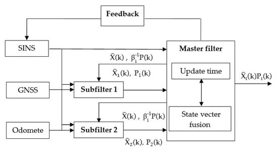
Figure 4. Federated filter architecture.

3.6.2. State Vector Fusion Process

State vector fusion means that the local state estimation of the Kalman filter of each subsystem is fused to obtain the global state estimation. After adopting the “upper bound of variance” technique, the measurement update and time update of each subfilter were performed independently, that is, the local estimation of each subfilter was irrelevant, so there was a state vector fusion algorithm.

When the state vector of each subfilter is the same, the global state estimate of the federated filter is the weighted average of the local estimates of the state vectors of all subfilters. The inverse of the positive definite symmetric weighting matrix is the sum of the inverse matrices of the covariance matrix$,{ \mathrm{P}}_{\mathrm{i}}\left(\mathrm{k}\right)\left(\mathrm{i}=1,2\right)$of each subfilter state estimation error. The globe state estimation equation is as follows:

$$\widehat{\mathrm{X}}\left(\mathrm{k}\right)={\left[{\displaystyle \sum }_{\mathrm{i}=1}^2{\mathrm{P}}_{\mathrm{i}}^{-1}\left(\mathrm{k}\right)\right]}^{-1}\left[{\displaystyle \sum }_{\mathrm{i}=1}^2{\mathrm{P}}_{\mathrm{i}}^{-1}\left(\mathrm{k}\right){\widehat{\mathrm{X}}}_{\mathrm{i}}\left(\mathrm{k}\right)\right]$$

(26)

The global state estimation error covariance is as follows:

$$\mathrm{P}\left(\mathrm{k}\right)={\left[{\displaystyle \sum }_{\mathrm{i}=1}^2{\mathrm{P}}_{\mathrm{i}}^{-1}\left(\mathrm{k}\right)\right]}^{-1}$$

(27)

3.6.3. Information Fusion Process

The federated filter global state estimation $\widehat{\mathrm{X}}\left(\mathrm{k}\right)$ and covariance matrix $\mathrm{P}\left(\mathrm{k}\right)$ reset the state estimation ${\widehat{\mathrm{X}}}_{\mathrm{i}}\left(\mathrm{k}\right)$ and covariance matrix${ \mathrm{P}}_{\mathrm{i}}\left(\mathrm{k}\right)$of the subfilter so that the subfilter can update recursively according to the following relationship:

$${\widehat{\mathrm{X}}}_{\mathrm{i}}\left(\mathrm{k}\right)=\widehat{\mathrm{X}}\left(\mathrm{k}\right)$$

(28)

$${\mathrm{P}}_{\mathrm{i}}\left(\mathrm{k}\right){=\mathsf{\beta }}_{\mathrm{i}}^{-1}\mathrm{P}\left(\mathrm{k}\right)$$

(29)

According to the principle of information conservation, the information distribution coefficient should satisfy the following condition:

$${\displaystyle \sum }_{\mathrm{i}=1}^2{\mathsf{\beta }}_{\mathrm{i}}=1$$

(30)

Different ${\mathsf{\beta }}_{\mathrm{i}}$can obtain different federated filter structures and characteristics (fault tolerance, accuracy, and calculation amount). The better the performance of the sub-navigation system, the larger the corresponding information distribution coefficient.

3.6.4. Information Distribution Method Based on Orthogonality of Innovation and Piecewise Smooth Activation Function

The working scene of the track detector often has a large number of unfavorable factors such as water area, mountains, tunnels, high-voltage cables, etc. It is therefore easy for the signal of a satellite positioning system to lose its lock through a multipath effect or electromagnetic interference, which can lead to noise in the output. The reliability of the measurement of the satellite positioning system is proportional to the dilution of precision (DOP) value of the satellite signal, where a smaller DOP indicates higher accuracy [34,35]. In this article, according to the nature of innovation orthogonality, the DOP value was used to judge whether each component of the quantity measurement was an outlier, and this information was then used to determine the information distribution coefficient.

The noise variance measurement and the DOP value have the following relationship:

$${\mathrm{R}}_{\mathrm{i}}{=\mathrm{N}}_{\mathrm{i}}{\mathrm{DOP}}_{\mathrm{i}}{+\mathrm{R}}_{\mathrm{i}0}$$

(31)

where ${\mathrm{R}}_{\mathrm{i}}$ is credibility of the ${\mathrm{i}}_{th}$ observed quantity, ${\mathrm{N}}_{\mathrm{i}}$ is the scaling factor of the satellite positioning system signal precision and the signal DOP value, and ${\mathrm{R}}_{\mathrm{i}0}$is adjustment amount for noise measurement.

The information allocation coefficient was determined by the piecewise smooth activation function shown in the following equation:

$${\mathrm{f}}_{\mathrm{i}}\left({\mathrm{r}}_{\mathrm{i}}\right)=\{ \begin{array}{c} 1 {\mathrm{r}}_{\mathrm{i}}\ll {\mathrm{d}}_{\mathrm{i}}\\ {\mathrm{d}}_{\mathrm{i}}/{\mathrm{r}}_{\mathrm{i}} {\mathrm{r}}_{\mathrm{i}}>{\mathrm{d}}_{\mathrm{i}}\end{array} \mathrm{i}=1,2,\cdots ,\mathrm{m}$$

(32)

$\mathrm{where} {\mathrm{r}}_{\mathrm{i}}$ and ${\mathrm{d}}_{\mathrm{i}}$ are obtained from ${\mathrm{R}}_{\mathrm{i}}$. The specific derivation and calculation process are detailed in [28].

The state vector fusion shown in Equation (32) occurs when the measurement is not an outlier, the gain of activation function is 1, and the information distribution coefficient ${\mathsf{\beta }}_1$= 1. When the measurement is an outlier$({\mathrm{r}}_{\mathrm{i} }{>\mathrm{d}}_{\mathrm{i}}$ and the activation function < 1, according to the dilution of precision of current measurement), the weighted distribution of ${\mathsf{\beta }}_1$and ${\mathsf{\beta }}_2$ in different precision ranges is realized.

4. Data Smoothing Algorithm

To realize the high-accuracy measurement of track geometry parameters using the inertial track geometry state detector, motion parameter measurement of the inertial/GNSS/odometer integrated navigation system is required to provide both high absolute and relative accuracy. The forward and reverse navigation solutions of the inertial navigation system are equivalent, whereas the traditional Kalman filter only uses data from the current filtering time and before filtering. Therefore, if all data from the navigation solution process can be used, the accuracy of the integrated navigation can be improved and the detection accuracy of the inertial track geometric state detector can be increased.

In this study, the forward filtering and the Rauch–Tung–Striebel (RTS) fixed interval smoothing algorithm [36,37,38] were adopted to achieve data smoothing processing for the entire navigation calculation process. The basic principle of the RTS algorithm is that a fixed interval is selected, and the forward solution is based on the Kalman filter. Then, based on all of the forward solution state variables of the fixed interval, the state of each data node in the fixed interval is reverse estimated, resulting in superior data accuracy to that of the forward filter [39,40,41].

The RTS fixed interval smoothing algorithm estimates the state of each data node based on all measurement information in a fixed interval. Suppose that in a fixed interval, there are N observations. First, based on the forward Kalman filter, the K = 1, 2, …, N combination filtering is carried out, and state estimation information $\widehat{\mathrm{X}}\left(\mathrm{k}\right)$, error estimation covariance matrix ${\mathrm{P}}_{\mathrm{k}}$, and one-step prediction error variance matrix ${\mathrm{P}}_{\mathrm{k}/\mathrm{k}-1}$ of N times combined filtering are stored. Then, following the forward Kalman filter in a fixed interval, and based on the stored combined filtering information, RTS reverse smoothing filtering is carried out according to the sequence K = N, N − 1, …, 1.

The RTS fixed interval inverse smoothing algorithm is as follows:

$${\widehat{\mathrm{x}}}_{\mathrm{k}-1/\mathrm{N}}={\widehat{\mathrm{x}}}_{\mathrm{k}-1}{+\mathrm{A}}_{\mathrm{k}-1}({\widehat{\mathrm{x}}}_{\mathrm{k}/\mathrm{N}}-{\mathsf{\Phi }}_{\mathrm{k}/\mathrm{k}-1}{\widehat{\mathrm{x}}}_{\mathrm{k}-1})$$

(33)

$${\mathrm{P}}_{\mathrm{k}-1/\mathrm{N}}{=\mathrm{P}}_{\mathrm{k}-1}{+\mathrm{A}}_{\mathrm{k}-1}{(\mathrm{P}}_{\mathrm{k}/\mathrm{N}}-{\mathrm{P}}_{\mathrm{k}/\mathrm{k}-1}{)\mathrm{A}}_{\mathrm{k}-1}^{\mathrm{T}}$$

(34)

The data smooth gain matrix is obtained as follows:

$${ \mathrm{A}}_{\mathrm{k}-1}{=\mathrm{P}}_{\mathrm{k}-1}{\mathsf{\Phi }}_{\mathrm{k}/\mathrm{k}-1}^{\mathrm{T}}{\mathrm{P}}_{\mathrm{k}/\mathrm{k}-1}^{-1}$$

(35)

5. Development and Accuracy Verification of Track Geometry State Detector Based on an Inertial/GNSS/Odometer Integrated Navigation System

5.1. Hardware Scheme of Inertial Track Geometry State Detector

As shown in Figure 5, the inertial track geometry state detector system was composed of six parts including an inertial measurement unit, odometer, satellite positioning system, gauge measuring instrument, data computer, and vehicle body. The inertial measurement unit (IMU) was rigidly connected to the car body and was used to measure the motion parameters of the railway track geometry state detector in the course of orbit operation. The IMU is the core component of the integrated navigation system. The odometer was fixed to the vehicle body motion wheel to measure the speed information of the vehicle body. The satellite positioning system used a single antenna scheme, which was fixed to the vehicle body to provide high-accuracy vehicle position and speed information. The high-accuracy linear variable differential transformer distance measurements were used to determine the track gauge values. A data computer was used for the acquisition, storage, and processing of the sensor data.

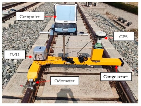
Figure 5. The composition of the inertial track geometry state detector system.

The overall weight of the railway track inspection instrument with a split design structure was 37 kg, and an operator is easily able to assemble and disassemble the instrument. The instrument is driven by the operator on foot, and the design speed is less than 8 km/h. Using a multisensor time synchronization mechanism, the data for the inertial measurement unit, satellite positioning system, odometer, and gauge measuring instruments are collected and joined. Then, the track geometry parameters are calculated using post-processing software. The main components and technical indicators of the inertial track geometry state detector are shown in Table 1.

Table 1. The main components and technical indicators of the inertial track detector.

Component	Model	Qualification	Parameter
Laser Gyroscope	HT-50TM	Zero Bias Stability	≤0.01 °/h
		Zero Bias Repeatability	≤0.01 °/h (1σ)
Accelerometer	JN-06M	Monthly repeatability of deviation	≤20 μg
I/F Conversion Circuit	GZH-06	Scale Factor Nonlinearity	≤1 × 10−4
		Zero Bias	≤0.5 Hz
GPS	OEM719	Data Update Rate	50 Hz
Odometer	EC50P-5000	Resolution	<0.002
Displacement Transduce	SDVH20	Resolution	≤0.1 μm

5.2. Software Scheme of Track Geometry State Detector

The data processing software of the track geometry state detector system was divided into four software modules: The sensor original data preprocessing module, the inertial navigation initial alignment module, the inertial/GNSS/odometer Kalman filter integrated navigation and reverse smoothing module, and the track geometry parameter calculation module, as shown in Figure 6.

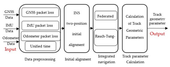
Figure 6. Design of data processing software for track inspector system.

5.3. Detection Accuracy Results and Analysis of Inertial Track Geometry State Detector

5.3.1. Selection of Test Field and Establishment of Test Reference

For this experiment, a continuous track with a length of about 1 km, which contained a straight line, transition curve, and circular curve, was selected as the standard test line following [42]. A permanent CPIII control network was established on the line, and the relative accuracy of CPIII points met the requirements of plane ± 1.0 mm and elevation ± 0.5 mm.

The line test was repeated and accurately measured three times using an Amberg GRP1000 type track geometry state detector, which has a detection accuracy of more than 1 mm. The average of the three test results obtained by the GRP1000 was used as a reference value for this test.

5.3.2. Measurement Accuracy Repeatability Test

The line test was repeated and accurately measured three times under the same environmental conditions using the inertial track geometry detector at a speed of 3 km/h. Based on the data processing software of the inertial detector system developed in this study, the data for the test line were processed, and the track geometry parameters of the test line were obtained. For the detection accuracy analysis, we examined and compared the geometric parameters of track direction, high and low, and horizontal (ultra-high). It should be noted that track gauge, track gauge change rate, and mileage can be measured by a track gauge sensor and mileage sensor on the inertial detector, so they were not analyzed in this study. For the convenience of comparative analysis, this test only used the measurement results for the track geometric parameters of the double-wheel side reference track for comparison. The track geometric parameters of the single-wheel side track could be calculated using the geometric parameters of the double-wheel side track, and the accuracy level is consistent.

The repeatability comparison of the three repeated detection datapoints of the track direction (high and low, and horizontal (ultra-high)) parameters of the test line are shown in Figure 7. Figure 7a–c show the real value of the track direction, high and low, and horizontal (ultra-high) parameters obtained from the three repeated detections of the test line. Figure 7b shows the difference between the second and third measurement results and the first measurement results in the track direction, high and low, and horizontal (ultra-high) parameter data obtained. It can be seen from Figure 7 that the repeatability error of the track direction, high and low, and horizontal (ultra-high) parameters detected by the inertial track geometry state detector based on inertial/GNSS/odometer integrated navigation was better than 0.2 mm, which shows an improved accuracy of the inertial track geometry state detector system.

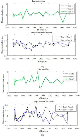
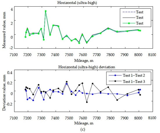
Figure 7. Repeatability comparison showing data from three experimental replicates for track geometry parameter measurements of test lines: (a) track direction; (b) high and low; (c) horizontal (ultra-high).

5.3.3. Accuracy Consistency Analysis of Track Geometric Parameter Detection

The line test was repeated and accurately measured three times using an Amberg GRP1000 type track geometry state detector. The displacement sensor for measuring the gauge and the tilt sensor for measuring the level were built into the detector. The total station was placed statically near the center of the measured track, and 6–8 control points were surveyed. The total station coordinates were obtained based on the resection algorithm. In the total station survey, the prism was placed on the track detector to obtain its three-dimensional coordinates. After obtaining all of the measurement data in this mode for each sleeper, the three-dimensional coordinates of the two rails and the track centerline could be derived based on the mechanical parameters calibrated in advance by the track detector. The average of the three test results obtained by the GRP1000 was used as a reference for this test.

The absolute deviation comparison of the track direction, high and low, and horizontal (ultra-high) parameters of the three repeated tests’ data is shown in Figure 8. Figure 8a shows the track direction, high and low, and horizontal (ultra-high) parameters obtained by the inertial detector for the three repeated detections of the test line and the detection results of the GPR1000 detector. Figure 8b shows the difference between the track direction, high and low, and horizontal (ultra-high) parameters obtained by the three repeated tests and the test results of the GPR1000 detector. As can be seen from Figure 8, compared with the results of the GPR1000 detector, the error in the track direction, high and low, and horizontal (ultra-high) parameters detected by the inertial detector based on the inertial/GNSS/odometer combined navigation was better than 0.2 mm, which improved the accuracy of the inertial track geometry state detector system.

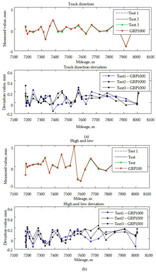
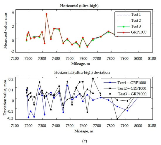
Figure 8. Absolute deviation comparison of three replicates of test data for track geometry parameters of test lines: (a) track direction; (b) high and low; (c) horizontal (ultra-high).

5.3.4. Test Results Comparison

Since 2013, many similar experiments have been conducted on the same test site, and the experimental results have been published in the literature [27,28,29]. After using the new filter proposed here, the measurement accuracy of the track geometry parameters of the track detector was improved. In order to better compare results, different algorithms were used to calculate the same data. The comparison is shown in Table 2.

Table 2. Comparison of measurement accuracy of different filtering methods.

Track Geometry Parameters	Measurement Accuracy by Centralized Filtering	Measurement Accuracy by Federated Filtering
Track direction	≤0.33 mm	≤0.2 mm
High and low	≤0.45 mm	≤0.2 mm
Horizontal (ultra-high)	≤0.31 mm	≤0.2 mm

The following are prospects for further work to build on our findings:

• Continue to study the inertial/GNSS/odometer integrated navigation post-filtering algorithm. This algorithm is the core of the inertial/GNSS/odometer integrated navigation system and the key to improving its accuracy. The attitude calculation accuracy of the integrated navigation system has already been improved.
• The next step is to carry out research on the detection and correction methods of data outliers and noise of the four types of sensors (gyroscope, accelerometer, satellite positioning system, and odometer), control the noise from the source, and improve the accuracy of the inertial/GNSS/odometer integrated navigation system.
• In the future, the federated filtering algorithm should be tested for computing power and fault tolerance using longer line sets and more data.

6. Conclusions

In this paper, the error equation of an inertial/GNSS/odometer integrated navigation system was derived, and the error models of the strapdown inertial navigation system and inertial/odometer dead reckoning were established. The federated Kalman filter architecture was established to estimate the system error, and the system error was then corrected using feedback. A data-smoothing algorithm based on forward filtering and reverse smoothing was used to improve detection accuracy. A novel inertial track geometry state detector was developed, and the feasibility and detection accuracy of the integrated navigation scheme were verified through on-track experiments. The main conclusions of this study are as follows:

• The information distribution coefficient of the state vector fusion algorithm is determined based on the orthogonality of innovation and the DOP value of the satellite signal, which improves the detection accuracy of the inertial track detector.
• The data-smoothing algorithm based on forward filtering and reverse smoothing improved the accuracy of integrated navigation and improved the detection accuracy of the inertial trajectory geometry state detector.
• A high-speed railway track geometry parameter tester system was constructed and developed. The measurement accuracy of the track geometry parameters was better than 0.2 mm, and the detection speed was about 3 km/h, which meets the requirements of high accuracy and high efficiency of high-speed railway track geometry detection.

In engineering practice, using the inertial track geometric state detection method proposed by this paper can realize the high-accuracy and high-efficiency geometry detection of an operating high-speed railway. This approach can also be extended to the maintenance of railways of varying speeds and long-track fine adjustment measurement of newly-built railways.

References

- Sánchez, A.; Bravo Trinidad, J.L.; González Ramiro, A. Estimating the accuracy of track-surveying trolley measurements for railway maintenance planning. J. Surv. Eng. 2016, 143, 5016008. [Google Scholar] [CrossRef]
- Li, Q.; Mao, Q. Progress on dynamic and precise engineering surveying for pavement and task. Acta Geodaetica et Geophysica Sinica 2017, 46, 1734–1741. [Google Scholar] [CrossRef]
- Li, Q.; Bai, Z.; Li, Q.; Wu, F.; Chen, B.; Xin, H.; Cheng, Y. Geometric design of an outdoor three-dimensional kinematic verification field for a position and orientation system. Sci. Technol. 2019, 59, 895–901. [Google Scholar] [CrossRef]
- Liu, W.; Tu, W.; Yang, F.; Yang, Z. Research on integrated inspection and monitoring system of high speed railway infrastructure. China Railw. 2019, 22–26. [Google Scholar] [CrossRef]
- BSI. Railway applications/Track-track geometry quality-Part 1: Characterisation of track geometry. In BS EN 13848-1:2003+A1:2008; British Standards Institution: London, UK, 2008. [Google Scholar]
- NRA. Administrative Measures for the Construction Safety of Railway Business Lines. In Rail Transport (2012) No.280; China Railway Press: Beijing, China, 2012. [Google Scholar]
- NRA. Railway Line Repair Rules. In Rail Transport (2006) No.146; China Railway Press: Beijing, China, 2006. [Google Scholar]
- Han, F. Research on the Status Detection and Evaluation Technology of Existing Railway Based on Point cloud information. Ph.D. Thesis, Southwest Jiaotong University, Chengdu, China, 2014. [Google Scholar]
- Luo, L.; Zhang, G.; Wu, W.; Chai, X. Control. of Track Smoothness of Wheel-Rail System; China Railway Press: Beijing, China, 2006; pp. 1–286. [Google Scholar]
- She, Y. Track Geometric State Inspection of High-Speed Railway by Vehicle-Borne Close-Range Photogrammetry. Master’s Thesis, Southwest Jiaotong University, Chengdu, China, 2014. [Google Scholar]
- Hong, S. Study on the Measurement Method of Track Inspection Car. Master’s Thesis, Guangdong University of Technology, Chengdu, China, 2015. [Google Scholar]
- Chen, Q. Research on the Railway Track Geometry Surveying Technology Based on Aided INS. Ph.D. Thesis, Wuhan University, Wuhan, China, 2016. [Google Scholar]
- Wu, W. Research on the Precision Measurement Method of Ballastless Track Based on the Vehicle ETS without Leveling in High-Speed Railway. Ph.D. Thesis, Nanchang University, Nanchang, China, 2018. [Google Scholar]
- Bai, H.; Zhang, F.; Zhang, W. Rapid Measuring Instrument for Track Geometric State. China Patent CN201520215786.9, 10 April 2015. [Google Scholar]
- Wildi, T.; Glaus, R. A Multisensor Platform for Kinematic Track Surveying. In Proceedings of the 2nd Symposium on Geodesy for Geotechnical and Structural Engineering, Berlin, Germany, 21–24 May 2002; pp. 1–10. [Google Scholar]
- Akpinar, B.; Gülal, E. Railway track geometry determination using adaptive Kalman filtering model. Measurement 2013, 46, 639–645. [Google Scholar] [CrossRef]
- Akpinar, B.; Gülal, E. Multisensor railway track geometry surveying system. IEEE Trans. Instrum. Meas. 2012, 61, 190–197. [Google Scholar] [CrossRef]
- Wei, H. Research on the Track Irregularities Survey Theory and Relevant Adjustment Technologies of HSR Track. Ph.D. Thesis, Nanchang University, Nanchang, China, 2014. [Google Scholar]
- Fu, Q.; He, F.; Li, S.; Fan, S.; Peng, C. New Type Track Inspection Instrument. China Patent CN200620035696.2, 25 September 2006. [Google Scholar]
- Tang, W. GJY-T-4 Type Track Inspection Instrument Adjustment Circuit Design. Master’s Thesis, University of Electronic Science and Technology of China, Chengdu, China, 2010. [Google Scholar]
- Yu, W. Research on the Data Processing Technology of the Second-Generation Track Inspection Instrument. Master’s Thesis, Nanchang University, Nanchang, China, 2009. [Google Scholar]
- Han, Y. A Combined Satellite Navigation and Inertial Measurement Orbit Measurement System and Method. China Patent CN201310014507.8, 15 January 2013. [Google Scholar]
- Han, Y. GPS Track Irregularity Detection System and Detection Method. China Patent CN201010230227.7, 19 July 2010. [Google Scholar]
- Chen, Q.; Niu, X.; Zuo, L.; Zhang, T.; Xiao, F.; Liu, Y.; Liu, J. A railway track geometry measuring trolley system based on aided INS. Sensors 2018, 18, 538. [Google Scholar] [CrossRef]
- Li, Q.; Bai, Z.; Chen, B.; Guo, J.; Xin, H.; Cheng, Y.; Li, Q.; Wu, F. A novel track measurement system based on GNSS/INS and multisensor for high-speed railway. Acta Geodaetica et Geophysica Sinica 2020, 49, 569–579. [Google Scholar] [CrossRef]
- Gao, Z.; Ge, M.; Li, Y.; Shen, W.; Zhang, H.; Schuh, H. Railway irregularity measuring using Rauch-Tung-Striebel smoothed multi-sensors fusion system: Quad-GNSS PPP, IMU, odometer, and track gauge. Gps. Solut. 2018, 22. [Google Scholar] [CrossRef]
- Zhan, X.; Cui, X. Two-position Alignment Method for Inertial Navigation System of Rail Tester. Bull. Surv. Mapp. 2017, 3, 5–8. [Google Scholar]
- Zhang, X.; Cui, X.; Yan, D. Application of modified Kalman filtering restraining outliers based on orthogonality of innovation to track tester. In Proceedings of the 13th IEEE International Conference on Mechatronics and Automation, IEEE ICMA 2016, Beijing, China, 1 January 2016; pp. 171–175. [Google Scholar]
- Zhang, X.; Cui, X. Zero velocity attitude correction for railway tracks geometry measurement by inertial system. Sci. Surv. Mapp. 2017, 42, 17–21. [Google Scholar]
- Suhr, J.K.; Jang, J.; Min, D.; Jung, H.G. Sensor fusion-based low-cost vehicle localization system for complex urban environments. IEEE Trans. Intell. Transp. Syst. 2017, 18, 1078–1086. [Google Scholar] [CrossRef]
- Meng, X.; Wang, H.; Liu, B. A robust vehicle localization approach based on GNSS/IMU/DMI/LiDAR sensor fusion for autonomous vehicles. Sensors 2017, 17, 2140. [Google Scholar] [CrossRef] [PubMed]
- Liu, X.; Liu, X.; Song, Q.; Yang, Y.; Liu, Y.; Wang, L. A novel self-alignment method for SINS based on three vectors of gravitational apparent motion in inertial frame. Measurement 2015, 62, 47–62. [Google Scholar] [CrossRef]
- Yongyuan, Q. Inertial Navigation (Version 2); Science Press: Beijing, China, 2014; pp. 1–376. [Google Scholar]
- Liu, W.; Wu, J. The Analysis of satellite visibility and DOP value of GPS and Compass Navigation Systems. In Proceedings of the 3rd Annual China Satellite Navigation Academic Conference, Guagnzhou, China, 15–19 May 2012. [Google Scholar]
- Gao, J.; Fang, Y.; Yang, Z.; Zhang, Z. The Simulation Analysis of GLONASS and GPS Based on STK. Sci. Technol. Eng. 2011, 11, 3384–3387. [Google Scholar]
- Rauch, H.E.; Tung, F.; Striebel, C.T. Maximum likelihood estimates of linear dynamic systems. AIAA J. 1965, 3, 1445–1450. [Google Scholar] [CrossRef]
- Wu, X.T.; Yang, Y.; Gao, W.; Zhang, Z.S.; Pei, Z.; Peshekhonov, V.G. Attitude error compensation technology for inertial platform of airborne gravimeter based on RTS smoothing algorithm. In Proceedings of the 24th Saint Petersburg International Conference on Integrated Navigation Systems, ICINS 2017, Saint Petersburg, Russia, 1 January 2017. [Google Scholar]
- Wei, S.; Yan, J.; Teng, L. Research on high-precision INS/GPS integrated navigation offline data-processing algorithm. Comput. Simul. 2016, 33, 58–62. [Google Scholar] [CrossRef]
- Liu, J.; Yuan, X. The applicaiton of smoothing filter to GPS/INS integrated navigation system. Aerosp. Control. 1995, 36–42. [Google Scholar] [CrossRef]
- Bierman, G.J. A new computationally efficient fixed-interval, discrete-time smoother. Automatica 1983, 19, 503–511. [Google Scholar] [CrossRef]
- Gu, S.S.; Liu, J.Y.; Zeng, Q.H.; Lv, P. A Kalman filter algorithm based on exact modeling for FOG GPS/SINS integration. Optik 2014, 125, 3476–3481. [Google Scholar] [CrossRef]
- NRA. Dynamic detection and evaluation of track geometry state. In TB/T 3355-2014; China Railway Press: Beijing, China, 2014. [Google Scholar]
Publisher’s Note: MDPI stays neutral with regard to jurisdictional claims in published maps and institutional affiliations. |
© 2021 by the authors. Licensee MDPI, Basel, Switzerland. This article is an open access article distributed under the terms and conditions of the Creative Commons Attribution (CC BY) license (https://creativecommons.org/licenses/by/4.0/).