Abstract
Trains are used as the fastest mode of transportation for both people and cargo. The train moves along a special path called “rail”, where fatigue can be accumulated due to wheel-rail contact load as a result of continuous train operation. Consistent and regularly scheduled safety management is required since corrosion rate of the rails located on outside environment is very high. Researchers have actively investigated and developed rail defect inspection systems employing non-destructive techniques to address these problems. In particular, the eddy current inspection technique does not involve contact with the surface of the test specimen and offers the advantage of excellent rail defect detection sensitivity. Therefore, a 16 Channel array eddy current inspection device was developed to inspect the surface defects of the rail. An equation was derived to predict the correlation between the depth and phase of an artificial defect using the eddy current inspection device, and the derived equation was applied to the natural defect specimen.
1. Introduction
Trains are the fastest means of transportation on land, contributing greatly to industrial development. Railway tracks are required for trains to move, and rails are composed of supports, sleepers, and roadbeds to distribute the train’s load. Rails are constantly subjected to fatigue load due to friction with the wheels of the train, and defects in the rail occur because of corrosion caused by the external environment (climate, etc.) [1]. Various surface defects in rails occur most frequently during rolling stock operation, and internal defects may develop, which lead to accidents if maintenance, such as grinding, is insufficient or not performed in advance.
In general, a visual inspection method is used for inspecting rail defects. As a method in which inspectors walk around and check whether a defect has occurred in the rail, visual inspection makes it possible to easily perform defect inspection, even without proficiency. However, in land transport inspection, it is difficult to determine defects occurring inside the rail, and there is a limit to the area that can be inspected. Another non-destructive method of detecting defects is ultrasonic testing.
Ultrasonic flaw detection is a method of inspecting the inside of a rail with a wave generated by vibrating a specific material [2,3]. Inspection using ultrasound has developed to the stage where it is possible to check the inside of a rail with an image using phased arrays, but it has a disadvantage in that it is difficult to detect defects on the surface of the rail because of the flaw detection structure. In particular, it is impossible to detect squat-type defects that occur on the rail surface because the ultrasonic wave does not propagate because of the instantaneous void between the rail surface and the ultrasonic probe surface.
Eddy current flaw detection is a technique proposed to compensate for the shortcomings of visual inspection and ultrasonic inspection. The eddy current inspection technique is a contactless method in which a high-frequency alternating current is applied to generate a magnetic field to detect changes in impedance between a coil and the specimen or the changes in voltage induced in a coil [4,5,6].
Therefore, eddy current inspection can be used to inspect the inside of the rail, which gives it an advantage over visual inspection, and it can be used very usefully because it can inspect the surface area, which gives it an advantage over ultrasonic inspection [7,8]. In the eddy current inspection method, a Lissajous figure can be drawn using X data (resistance) and Y data (reactance), which are signal outputs from the sensor, and the size of a defect can be obtained using amplitude and phase [9,10].
Previously developed eddy current flaw detection equipment is designed in a structure that cannot inspect the entire head of the rail using a small number of sensors. In order to inspect the entire head of the rail, technology that can minimize the dead zone area using multiple eddy current sensors is required. Along with the minimization of the dead band region, the performance of the eddy current sensor also plays an important role. In general, an eddy current sensor consists of a coil, and since a coil that responds according to the direction of a defect is determined, a technology capable of inspecting all defects using one sensor is required.
In this study, the number of sensors was optimized by manufacturing a Plus-Point coil so that flaw detection could be performed regardless of the direction of the defect, and a total of 16 eddy current sensors were used to inspect the entire head of the rail. In addition, two-dimensional and three-dimensional rail surface shapes were obtainable through separate software, and a relational expression for analyzing the depth of the defect was derived by manufacturing artificial defects on the rail surface.
2. Defect Detection Technique Using Multi-Channel Eddy Current System
The multi-channel eddy current inspection system developed in this study was applied to investigate natural surface defects on a UIC 60 rail. The obtained signals were used to compare and evaluate the signal characteristics of the defects and compare them with the actual defects in 2D and 3D images to confirm the accuracy of the defect detection.
Figure 1 displays the analysis sequence for multi-channel eddy current testing. The X and Y data of natural rail defect test specimens were collected using a multi-channel sensor, and the data were subsequently subjected to a de-trending and de-noising process. It was possible to acquire the defect image after correcting the difference (amplitude and phase) between the sensors. The procedure is described in detail in Figure 1.
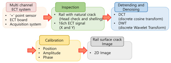
Figure 1.
Multi-channel ECT signal analysis.
2.1. 16 Ch Eddy Current Sensors
Plus-point sensors, which are a type of differential sensors, were used in this study [11]. The plus-point sensors crossed the “I”-shaped coils crosswise to differentially detect the defects; as the lift-off (the gap between the specimen and the sensor) changes, the crossed coils are simultaneously affected and canceled, thus minimizing the effect of lift-off and reducing noise [12,13]. Furthermore, defects in various directions rather than in one direction can be detected [14]. The plus-point sensors were fabricated with four layers (two layers each) with an outer diameter of 8 mm and a height of 30 mm.
The jig was constructed as shown in Figure 2a,b such that the 16 sensors could be secured and the entire rail surface could be inspected. The sensor spacing in the direction of rail propagation was set to 18 mm, and to inspect the entire rail head, the sensor spacing between the rail propagation direction and vertical direction was 3.8 mm, which resulted in a total of 57 mm. The jig to which the sensors were connected was divided into four parts and could be disassembled and reassembled. Four sensors were combined onto one jig apparatus, and the arrangement of the sensors could be changed by disassembling and reassembling the jig. Furthermore, a constant lift-off distance from the wheels attached to the jig to the rail surface could be maintained.
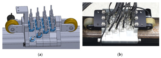
Figure 2.
Multi-channel ECT sensor jig: (a) jig design, (b) jig maked.
2.2. 16 Ch Eddy Current System
2.2.1. System Introduction
A power supply was used to apply 12 V of power to the 16-channel eddy current system. The 16-channel eddy current system distributes the supplied power and applies 7 V of power to the sensors; it is connected to the acquisition program through a LAN connection and stores the real-time monitoring data and the X and Y component signal outputs. The acquisition program can monitor 16 channels of X and Y signals and 2D images in real time, and it can create a 3D image of the section where a defect occurs. In addition, the frequency and gain value can be set. In the experiment, we applied a frequency of 300 kHz and lift-off of 1 mm.
2.2.2. Frequency Setting
In order to set the optimal frequency of the multi-channel eddy current system, the phase change was confirmed according to the frequency change, as shown in Table 1. When the amount of phase change is large, the resolution increases when converted to the depth of the defect, and the error of the defect decreases as the deviation value is minimized in the same defect. It was confirmed that the largest frequency change was measured at 300 kHz, and the deviation was minimized at 350 and 300 kHz. Therefore, 300 kHz was set as the optimal frequency for measuring defects.

Table 1.
Phase change according to frequency change.
2.3. Natural Crack Specimen
Natural defects occur because of rolling stock operation on the rail and cumulative tonnage (more than 500 million tons) and external environmental factors. Natural defects that occur in general are shown in Figure 3a,b. Figure 3a shows a head check defect on the rail surface, and Figure 3b shows a shelling defect on the rail surface.
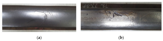
Figure 3.
Crack specimen: (a) head check and (b) shelling.
A head check occurs as a solid line resulting from slip and frictional stress between the rail and the wheel [15,16]. Shelling occurs because of the development of the head check; it is a defect in which the surface of the rail breaks shallowly because of the continuous load and friction of the train.
2.4. Calibration Data
2.4.1. Calibration Specimen
This study aimed to measure the defects occurring in the rail head using a 16 Ch eddy current sensor. However, since the 16 Ch eddy current sensor was manufactured by hand, a difference occurred in the amplitude measured by the sensor when passing through the same defect. In order to minimize the error between the sensors, a calibration test piece, as shown in Figure 4, was prepared. In order to ensure that all sensors passed through the same defect, the calibration test piece was manufactured with a defect that had a length of 1 mm and a depth of 3 mm over the entire head.
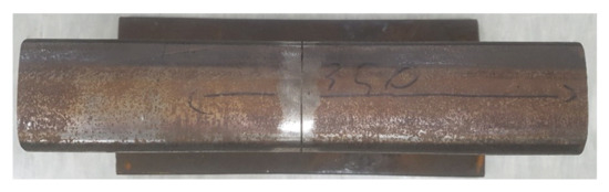
Figure 4.
Calibration specimen.
As shown in Figure 2 because the sensors are not on a straight line arranged in a 4 × 4 as shown in Figure 5a. Therefore, when scanning the test piece in Figure 4, it was possible to obtain the results shown in Figure 5a. Since the actual defect lay in a straight line, a position correction was required, and a calibration value that minimized the amplitude difference between sensors was required.
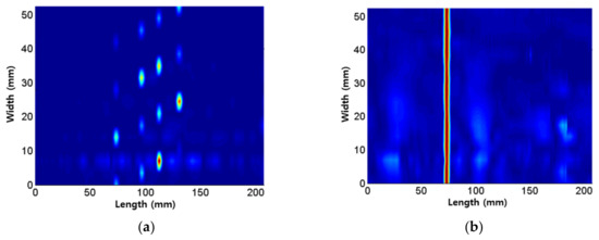
Figure 5.
Calibration: (a) before and (b) after.
- Calibration value measurement method (position and amplitude)
- (1)
- The defect location of each sensor is checked.
- (2)
- The sensor number that found the defect first is called “A1”.
- (3)
- The distance difference from each sensor to “A1” is called the position calibration value.
- (4)
- The amplitude of each sensor is checked.
- (5)
- The sensor number with the maximum amplitude is called “B1”.
- (6)
- The value is multiplied so that the amplitude of each sensor becomes “B1”, and this is called the amplitude calibration value.
Figure 5b shows the result of applying the calibration value, and it was confirmed that all had the same amplitude at the same location.
2.4.2. Signal Processing (Denoising and Detrending)
Figure 6 shows the raw data of the 16 Ch eddy current sensor passing the calibration test piece in Figure 4. Since only one defect existed in the calibration test piece, the amplitude change occurred once for each sensor. It can be seen that there was a difference in amplitude depending on the characteristics of each sensor and that sensors 4 and 8 generated a great deal of noise.
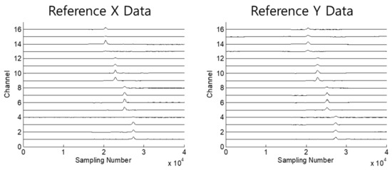
Figure 6.
Reference data.
Since the noise of the signal prevented the identification of the location of the defect or acted as an error in analyzing the size of the defect, noise removal was performed through denoising. The denoising technique used in this study was “DC Offect”, and signal processing was performed by applying data between the initially generated low frequency and a specific high frequency. Figure 7 shows the denoising process, and it was confirmed that the noise disappeared as a result of applying “DC Offect”.
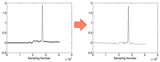
Figure 7.
Denoising process.
As can be seen in Figure 7, the denoising data had a certain tendency. Certain trends could also be viewed as noise, and detrending removed certain trends in the data. In this study, the “Polynomial Fitting—Bisquar and Givens” technique was used for detrending. Figure 8 shows the process of detrending the data of Ch4 after the denoising process.
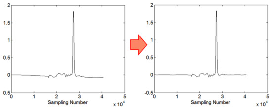
Figure 8.
Detrending process.
2.4.3. Cali Signal Correction Using Calibration Test Specimens
Table 2 shows the position, amplitude, and phase of the sensor from the calibration data obtained from Figure 8. The position was adjusted so that all defect signals could be acquired from the same position. The amplitude is the correction value used to make all sensors the same as they passed through the same defect. The phase must also have the same angle because all sensors pass through the same defect. The angle was set so that all sensors were set to 45°.
Table 2.
Calibration data set.
3. Depth Estimation of Artificial and Natural Defects
3.1. Multi-Channel Eddy Current System for Rail Surface Defect Inspection
In order to carry out the inspection at a long distance in the field, the equipment shown in Figure 9 was manufactured. The multi-channel sensor has 16 transducer channels built in, and the system is equipped with power and sensors for collecting signals, and the acquisition program can be installed on a tablet PC to lighten the equipment. The inspection speed of the equipment was set to 2 km/h, compliant with the average walking speed of most people.
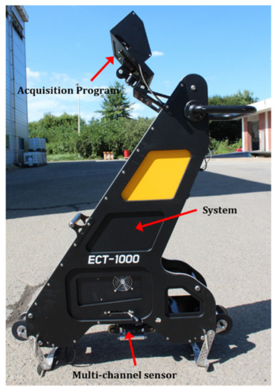
Figure 9.
Equipment used in the field.
3.2. Depth Estimation Using Artificial Defect Specimen
In order to derive the relationship between the depth and the phase of the defect, as shown in Figure 10, the artificial defect specimen was constructed with four squat defects on the UIC60 sample. The depths of the defects were 2, 4, 6, and 8 mm, and the lengths and widths were all 10 mm.
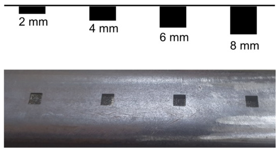
Figure 10.
Artificial defect depth change of the specimen.
Figure 11 shows the results of the scan of the artificial defect specimen. Figure 11a is the X data (resistance) of the eighth sensor, and Figure 11b is the Y data (reactance). As shown in Figure 11a,b, detrending and denoising were performed through signal processing. As a result of applying calibration, it was confirmed that two peaks were generated when the detector passed through the defect. These two peaks are the start- and endpoints of the defect, and the length of the defect can be measured using the two peak points.
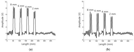
Figure 11.
Ch 8 Data: (a) X data (resistance) and (b) Y data (reactance).
The phase was used to estimate the depth of the defect. Figure 12 shows the relationship for estimating the depths of the defects, and Equation (1) shows the relationship between depth and phase. As a result of the measurement, it was confirmed that the phase increased at a constant rate as the depth of the defect increased.
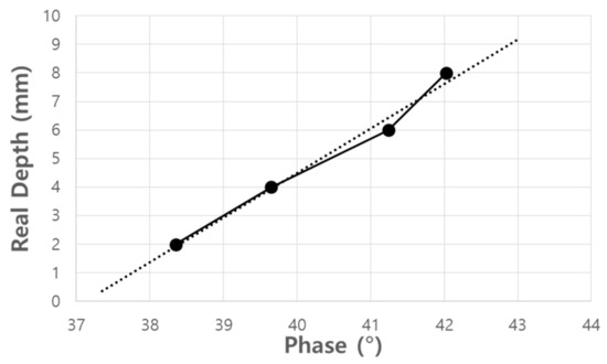
Figure 12.
Correlation between depth and phase.
Figure 13 shows the results of estimating the depth of artificial defects according to the depth change through a total of six repeated experiments. The red dotted line in Figure 13 is an error bar of ±1 mm, and it can be observed that there was no point beyond the error bar. Therefore, it is possible to estimate the depth of the surface defects of different specimens using the correlation between the depth and the phase of the derived defect.
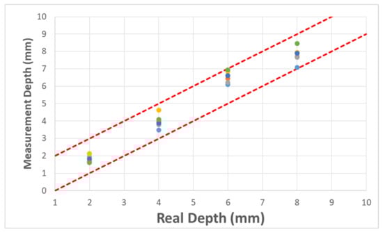
Figure 13.
Depth estimation result of the artificial defect specimen.
3.3. Natural Rail Defect Test Specimen Image
The calibration data in Table 1 were applied, and the results of the head check defect inspection shown in Figure 3a using the 16-channel sensors are shown in Figure 14. Figure 14a shows the X data (resistance), and Figure 14b shows the Y data (reactance). As shown in Figure 14a,b, the depth of the head check defect can be expected to vary because the X and Y signals are measured differently.
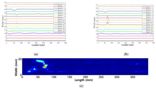
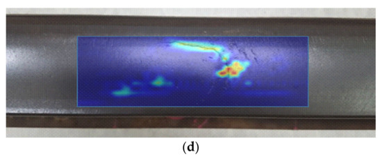
Figure 14.
Head check signal using 16 Ch array ECT sensor: (a) X data (resistance), (b) Y data (reactance), (c) 2D, and (d) real and result crack.
Figure 14c shows an image similar to the shape of the specimen as a result of calibration. The image shown in Figure 14d was used for an exact comparison by overlaying the defect part in Figure 14c with the image of the actual defects, and the results were shown to be consistent with head check defects.
The measurement was conducted a total of six times using a 16 Ch array eddy current device, and the average value of the phases was measured at 40.153°. As a result of the calculation by substituting the measured phase into Equation (1), the depth of the defect was 4.747 mm.
Figure 15a shows the image results after the shelling defect from Figure 3b was calibrated. The image shown in Figure 15b was used for an exact comparison by overlaying it with the image in Figure 15a with the actual defect, and the deep-pitched position was measured to be at a similar point, but not at the exact same position. The measurement was conducted a total of six times using a 16 Ch array eddy current device, and the average value of the phases was measured at 41.248°. As a result of the calculation by applying the measured phase to Equation (1), the depth of the defect was 6.454 mm.
Figure 15.
Shelling signal using 16 Ch array ECT sensor: (a) X data (resistance), (b) Y data (reactance).
4. Conclusions
In this study, an artificial defect was installed on the UIC60 rail surface, and using a 16-channel eddy current flaw detection system, a relational equation to analyze the depth was derived. In addition, two-dimensional and three-dimensional defect images could be acquired using the newly developed program.
Sensor calibration and signal processing techniques were used to improve the inspection accuracy and signals. The comparison of signal characteristics indicated that the peak width of the head check defect was narrower than the shelling defect. Two defect types (head check and shelling) were reproduced in 2D images, and the images were compared to the actual defects. The location and distribution of the defect signals in the images overlapped with those of the actual defects. Furthermore, the position of the defect and the area in which the defect propagated in the depth direction were confirmed, which could not be confirmed visually in the previous stages. The 3D images of the defects allowed us to confirm the signal size of the section in which the depth substantially increased as well as the surface roughness according to the degree of noise. The comparison of the 2D and 3D images using the 16-channel eddy current system with actual defects confirmed the detection accuracy.
Furthermore, to analyze the depth of defects, artificial defects were produced to derive the correlation between the defects and the phase. To confirm the reliability of the derived correlation, it was confirmed that the error range does not exceed ±1 mm through a number of experiments. It was confirmed that the depth can be analyzed using the correlation derived from the depth measurement of the natural defects.
The 16-channel eddy current flaw detection equipment can be used to measure defects on the rail surface, and it is expected to contribute to the stable management of rails by applying it to 50 K and 60 K specimens.
Author Contributions
S.-G.K. conceived and designed the experiments; S.-J.P., J.-W.P. and T.-G.L. performed the experiments; J.-M.S. and S.-G.K. analyzed the data; J.-M.S. and J.-W.P. performed experiments and analyzed data; S.-G.K., J.-M.S. and T.-G.L. wrote the paper. All authors have read and agreed to the published version of the manuscript.
Funding
This research received no external funding.
Institutional Review Board Statement
Not applicable.
Informed Consent Statement
Not applicable.
Data Availability Statement
Not applicable.
Conflicts of Interest
The authors declare no conflict of interest.
References
- Han, S.W.; Cho, S.H. Review of Non-Destructive Evaluation Technologies for Rail Inspection. J. Korean Soc. Nondestruct. Test. 2011, 31, 398–413. [Google Scholar]
- Kim, G.W.; Seo, M.K.; Kim, Y.I.; Kwon, S.G.; Kim, K.B. Development of phased array ultrasonic system for detecting rail cracks. Sens. Actuators A Phys. 2020, 311, 112086. [Google Scholar] [CrossRef]
- Heckel, T.; Thomas, H.M.; Kreutzbruck, M.; Rühe, S. High Speed Non-Destructive Rail Testing with Advanced Ultrasound and Eddy-Current Testing Techniques. Available online: https://opus4.kobv.de/opus4-bam/frontdoor/index/index/docId/20883 (accessed on 28 June 2021).
- Xu, P.; Zhu, C.L.; Zeng, H.M.; Wang, P. Rail crack detection and evaluation at high speed based on differential ECT system. Measurement 2020, 166, 108152. [Google Scholar] [CrossRef]
- Yu, Y.; Gao, K.; Liu, B.; Li, L. Semi-analytical method for characterization slit defects in conducting metal by Eddy current nondestructive technique. Sens. Actuators A Phys. 2020, 301, 111739. [Google Scholar] [CrossRef]
- Papaelias, M.P.; Lugg, M. Detection and evaluation of rail surface defects using alternating current field measurement techniques. Proc. Inst. Mech. Eng. Part F J. Rail Rapid Transit 2012, 226, 530–541. [Google Scholar] [CrossRef]
- Park, J.W.; Park, J.H.; Song, S.J.; Kishore, M.B.; Kwon, S.G.; Kim, H.J. Enhanced Detection of Defects Using GMR Sensor Based Remote Field Eddy Current Technique. J. Magn. 2017, 22, 531–538. [Google Scholar] [CrossRef]
- Garcia-Martin, J.; Gomez-Gil, J.; Vazquez-Sanchez, E. Non-Destructive Techniques Based on Eddy Current Testing. Sensors 2011, 11, 2525–2565. [Google Scholar] [CrossRef] [PubMed]
- Papaelias, M.P.; Roberts, C.; Davis, C.L. A review on non-destructive evaluation of rails: State-of-the-art and future development. Proc. Inst. Mech. Eng. Part F J. Rail Rapid Transit 2008, 222, 367–384. [Google Scholar] [CrossRef]
- Park, J.W.; Park, J.H.; Song, S.J.; Kim, H.J.; Kwon, S.G. GMR Sensor Applicability to Remote Field Eddy Current Defect Signal Detection in a Ferromagnetic Pipe. J. Korean Soc. Nondestruct. Test. 2016, 36, 483–489. [Google Scholar] [CrossRef][Green Version]
- Lee, T.G.; Yeom, Y.T.; Kim, H.J.; Song, S.J.; Kwon, S.G.; Kwon, S.D. Analysis of Eddy Current Signal of Defects on Railway. Korean Phys. Soc. 2019, 69, 361–368. [Google Scholar] [CrossRef]
- Sabbagh, H.A.; Sabbagh, E.H.; Murphy, R.K. Recent advances in modeling eddy-current probes. AIP Conf. Proc. 2002, 615, 423–429. [Google Scholar]
- Yusa, N.; Perrin, S.; Mizuno, K.; Chen, Z.; Miya, K. Eddy current inspection of closed fatigue and stress corrosion cracks. Meas. Sci. Technol. 2007, 18, 3403. [Google Scholar] [CrossRef]
- Lee, H.J.; Kim, Y.S.; Nam, M.W.; Yoon, B.S.; Kim, S.K. Eddy Current Testing of Weldment by Plus(+) Point Probe. J. Korean Soc. Nondestruct. Test. 1999, 19, 426–432. [Google Scholar]
- Seo, J.-M.; Kwon, S.-G.; Park, Y.-G. A Study on the Effect Analysis of Rail Grinding in Highspeed Railway considering Dynamic Wheel-Rail Force. J. Korean Soc. Railw. 2019, 22, 494–503. [Google Scholar] [CrossRef]
- Dwyer-Joyce, R.S.; Lewis, R.; Gao, N.; Grieve, D.G. Wear and Fatigue of Railway Track Caused by Contamination, Sanding and Surface Damage. In Proceedings of the 6th International Conference on Contact Mechanics and Wear of Rail/Sheel Systems: CM2003, Gothenburg, Sweden, 10–13 June 2003; pp. 211–220. [Google Scholar]
Publisher’s Note: MDPI stays neutral with regard to jurisdictional claims in published maps and institutional affiliations. |
© 2021 by the authors. Licensee MDPI, Basel, Switzerland. This article is an open access article distributed under the terms and conditions of the Creative Commons Attribution (CC BY) license (https://creativecommons.org/licenses/by/4.0/).