Article

A Finite Element Method to Predict the Mechanical Behavior of a Pre-Structured Material Manufactured by Fused Filament Fabrication in 3D Printing

1
ERMESS, EPF-Engineering School, 2 Rue Fernand Sastre, 10430 Rosières-prés-Troyes, France
2
Institut Charles Delaunay, LASMIS, UTT, UMR CNRS 6281, 12 Rue Marie Curie, 10010 Troyes, France
3
Institut Pascal CNRS-UMR 6602, Université Clermont Auvergne, PB 10448, 63000 Clermont-Ferrand, France
*
Author to whom correspondence should be addressed.
Appl. Sci. 2021, 11(11), 5075; https://doi.org/10.3390/app11115075
Submission received: 4 May 2021 / Revised: 27 May 2021 / Accepted: 27 May 2021 / Published: 30 May 2021
(This article belongs to the Special Issue Design for Additive Manufacturing: Methods and Tools)

Abstract

:
In this paper, a numerical method is proposed to simulate the mechanical behavior of a new polymeric pre-structured material manufactured by fused filament fabrication (FFF), where the filaments are oriented along the principal stress directions. The model implements optimized filament orientations, obtained from the G code by assigning materials references in mesh elements. The Gauss points are later configured with the physical behavior while considering a homogeneous solid structure. The objective of this study is to identify the elastoplastic behavior. Therefore, tensile tests were conducted with different filament orientations. The results show that using appropriate material constants is efficient in describing the built anisotropy and incorporating the air gap volume fraction. The suggested method is proved very efficient in implementing multiplex G code orientations. The elastic behavior of the pre-structured material is quasi-isotropic. However, the anisotropy was observed at the yield point and the ultimate stress. Using the Hill criterion coupled with an experimental tabular law of the plastic flow turns out to be suitable for predicting the response of various specimens.

1. Introduction

With the recent development in manufacturing techniques, smart materials become more effective at answering the requirement of highly advanced industrial applications. Those materials have the ability to react to external stimulations and can adapt their behavior according to the environment. This research constitutes a relatively recent area, which has emerged from the prospect of producing topologically optimized and complex shapes using additive manufacturing. In [1], Gardan defined a class of smart materials applied to additive manufacturing (AM) as follows: “advanced structured materials, which are based on a static definition of complex shapes or a material’s combination to achieve one or more properties that respond to a predefined functionality”.
The concept of designing advanced structures by AM materials is widely applied to enhance structural performance and manufacture custom materials with specific functionality. For instance, Li et al. [2] worked on a toughening method of fracture properties using 3D printed topological patterns on a sample surface which effectively delayed crack initiation and deflected crack propagation. In a like manner, Madugula et al. [3] proposed an optimization method that uses continuous extrusion in 3D printing. It consists of an iterative procedure using re-meshing and analysis by finite element simulations. The proposed approach was applied to enhance the strength of a four-point bending beam made with Polylactic Acid PLA material.
A new stress-based criterion for filament deposition in FFF FDM 3D printing has been suggested and tested [4]. The work reported herein is based on reproducing principal stress orientations in the sample to define the filament’s trajectory deposition in the manufacturing process. It was inspired by the reinforcement principle of composite materials where the fibers are oriented toward the in-plane tensile stress. Experimental studies have reported that this “enhanced” deposition method tested on an Acrylonitrile Butadiene Styrene (ABS) material generates an improvement by over 20% of fracture toughness and leads to a ductile-like fracture behavior [5,6,7]. In the same spirit, Kim et al. [8] developed a customized 3D printing tool-path for carbon fiber reinforced polymer where the carbon fibers reproduce the principal stress directions. This tool was used to print a spur gear geometry leading to a considerable improvement in the gear stiffness. The previously described deposition method has been proposed to surmount the problems caused by classical deposition methods such as layers alternation +45°/−45° or 0°/90° raster angle orientation. In those configurations, a locally heterogeneous structure is created because of the weld lines and the residual air gaps between the deposed filaments. These trajectories do not necessarily respect the use requirements of the part since a misplaced weld line, considered as a weakness, can lead to the reduction of the structure’s strength.
Materials fabricated by fused filament fabrication (FFF) are supposed to exhibit strong anisotropy due to the filaments’ orientation and the presence of an air gap [9]. Therefore, modeling their behavior will require a deep understanding of local phenomena occurring while loading the material. Rankouhi et al. [10] reveal the effect of the air-gaps size on the fracture morphology of the specimens announcing that larger air-gaps can cause inter-raster fusion bonds to fail which results in a more discretized surface area. In the study by Roy Xu et al. [11], a dual-notch void model was used to provide an explanation of the anisotropic tensile strengths of a 3D printed polymer. Most recently [12] Allum et al. demonstrated that the interface between layers in 3D printed PLA material has isotropic strength equivalent to that of the bulk filament. This study suggested that the anisotropy is caused by the welding lines’ geometries and a localized strain represented by a stress concentration. It opposes the assumption of the weaker behavior of weld lines. The previously mentioned studies stand as proof of the complexity of 3D printed parts behavior and reveal many issues to model such materials.
Numerous studies investigate the effect of raster orientation on the mechanical behavior of 3D printed parts through experimentation [13,14,15,16,17,18,19]. To investigate the orthotropic elastic properties of 3D printed parts, Biswas et al. [20] developed computational models based on microstructures of 3D printed ABS using micromechanics of a representative volume element (RVE). In a similar fashion, Nasirov et al. [21] employed asymptotic homogenization as a tool for predicting the mechanical properties of fused filament fabricated thermoplastics with line infill and grid infill structures. Both Ghandriz et al. [22] and Li et al. [2] used the extended finite element method (XFEM) with cohesive segments to capture the dependency of fracture behavior on build/raster orientations. The classical laminate theory was also utilized to model orthotropic mechanical properties of 3D printed parts [19,23].
Although research has illuminated the effect of raster orientation through different modeling methods and experimentation, no study to date has studied complex deposition trajectories. Previous studies have almost exclusively focused on modeling unidirectional or bidirectional raster orientations. No numerical study to date has examined complex deposition trajectories.
In this paper, the authors intend to propose a simplified finite element method that surmounts the weld lines and the air-gap problems by approaching the behavior in a global way. The model considers the material as homogenous and reproduces the built trajectories using local references assignment in the mesh element [24]. A transverse isotropic law is therefore defined at each integration point to model the behavior in the elastic region. The material constants were determined from a tensile specimen fabricated using the same parameters as the pre-structured material. Then, the Hill criterion coupled with a plastic flow model was identified to go until the fracture limit. The finite element software ABAQUS has been used to implement the identified elastoplastic behavior. Nevertheless, local phenomena such as filaments buckling and air gap repartition are not modeled. The related problems will be discussed later on where this numerical tool will be tested on the compact tension CT specimen [4] and the Single Edge Notched Bend SENB specimen defined in [7] where both the optimized deposition and the classical deposition trajectories will be modeled and compared.
The structure of the paper is as follows. In Section 2, the modeling strategy adopted for the 3D printed material is presented. First, the local references assignment technique is explained. Then the pre-structured material behavior definition is presented. Next, the experimental setups and results are displayed. In Section 4, the implementation of the material’s behavior in ABAQUS is detailed. In Section 5, the model will be used to predict the tensile tests. Afterward, it will be applied to the CT and SENB specimens. Here, its capability of implementing complex deposition trajectories will be checked and the limitations of the proposed method will be resumed in Section 6.

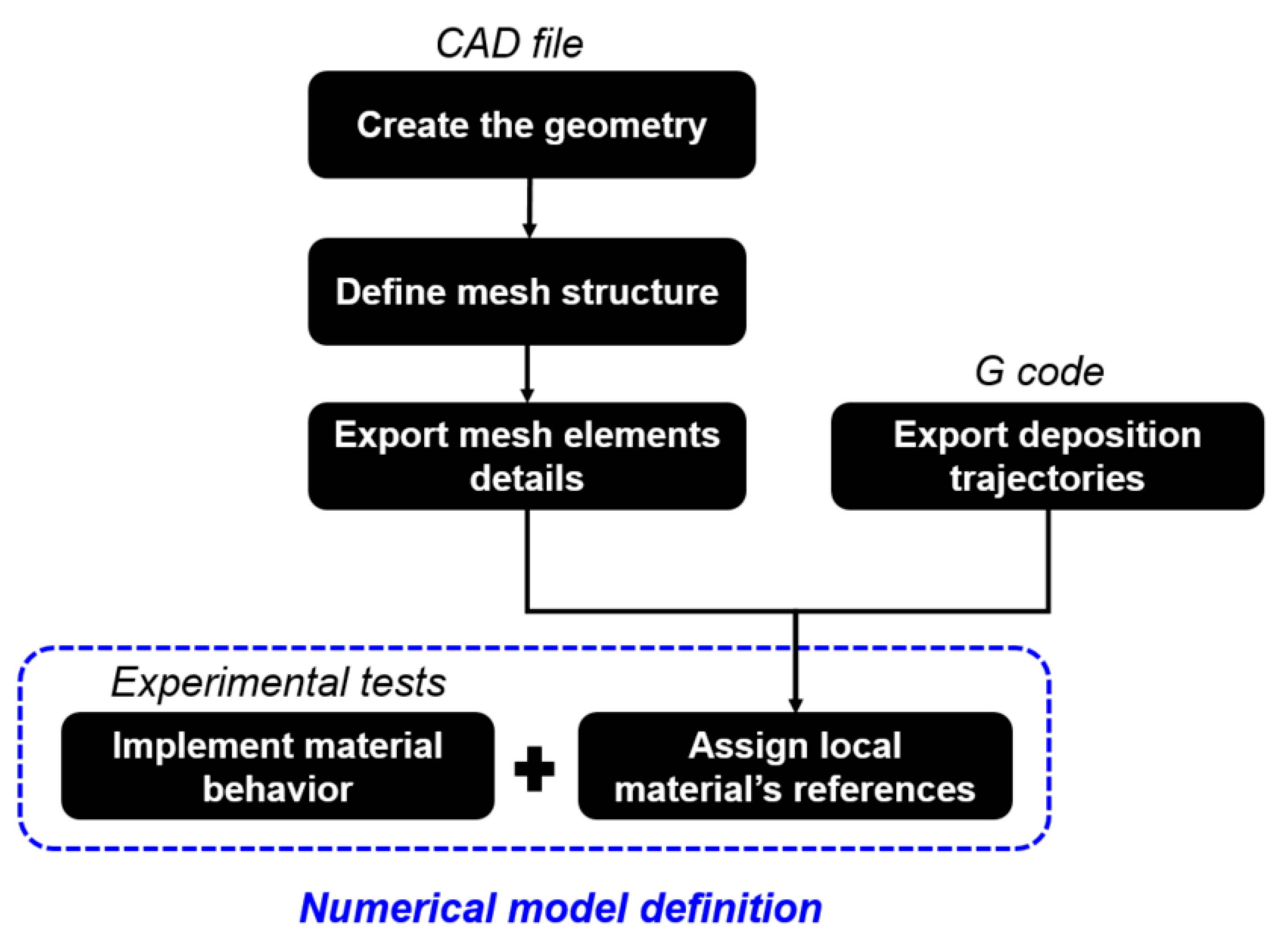
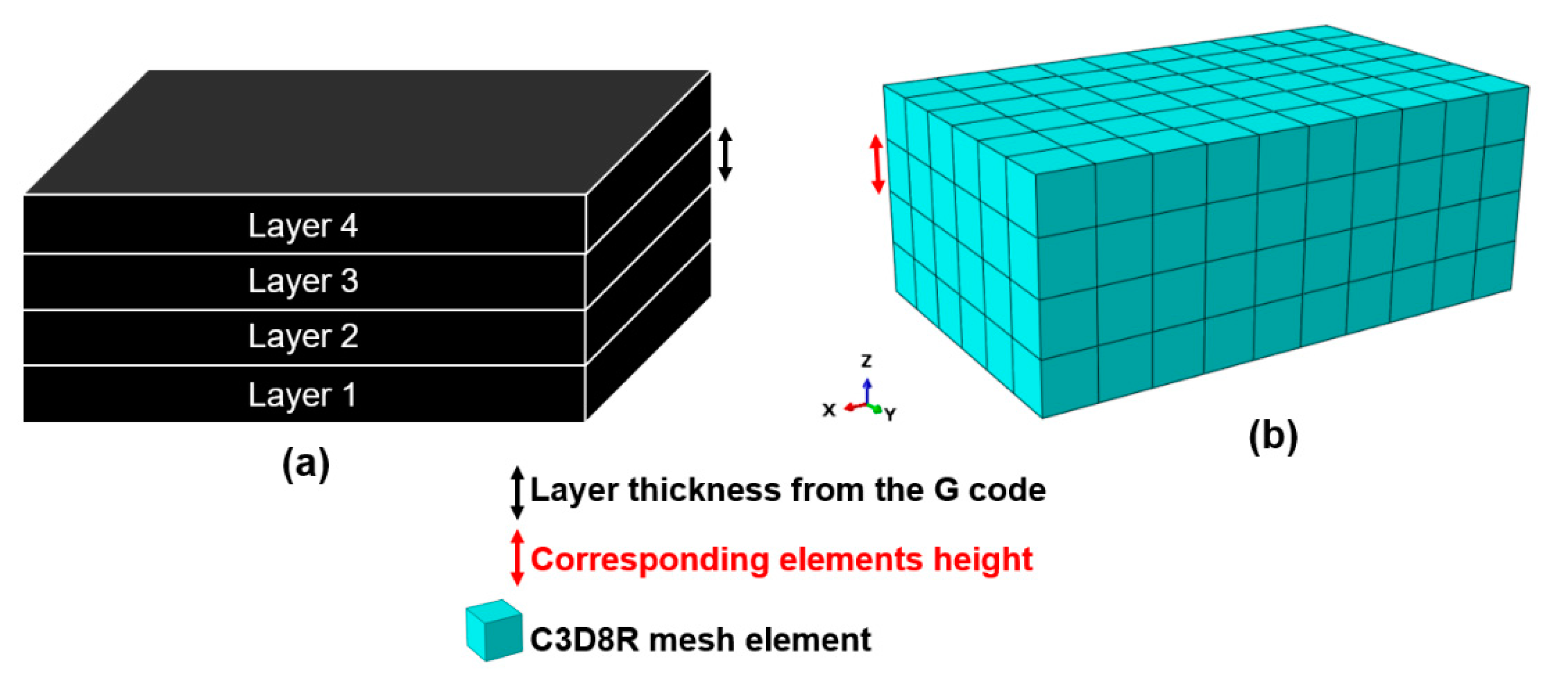
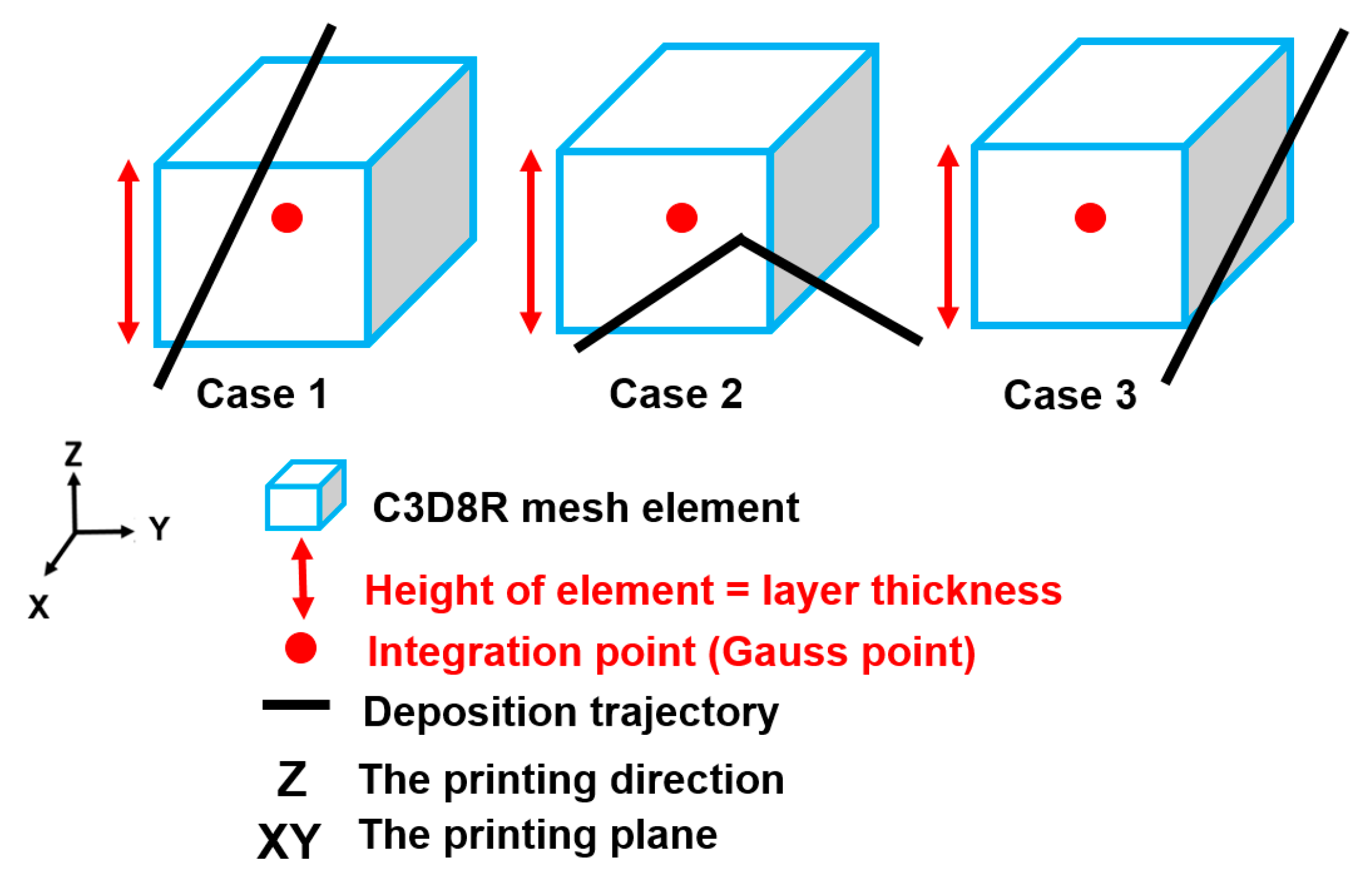
2. Modeling Methodology

The proposed modeling method is based on a simplification of the built configuration by considering a homogenous material. The complex structures containing the weld lines and the air gaps will be represented by implementing equivalent mechanical behavior constitutive equations. The developed workflow is presented in Figure 1 and will be detailed in the following subsections.

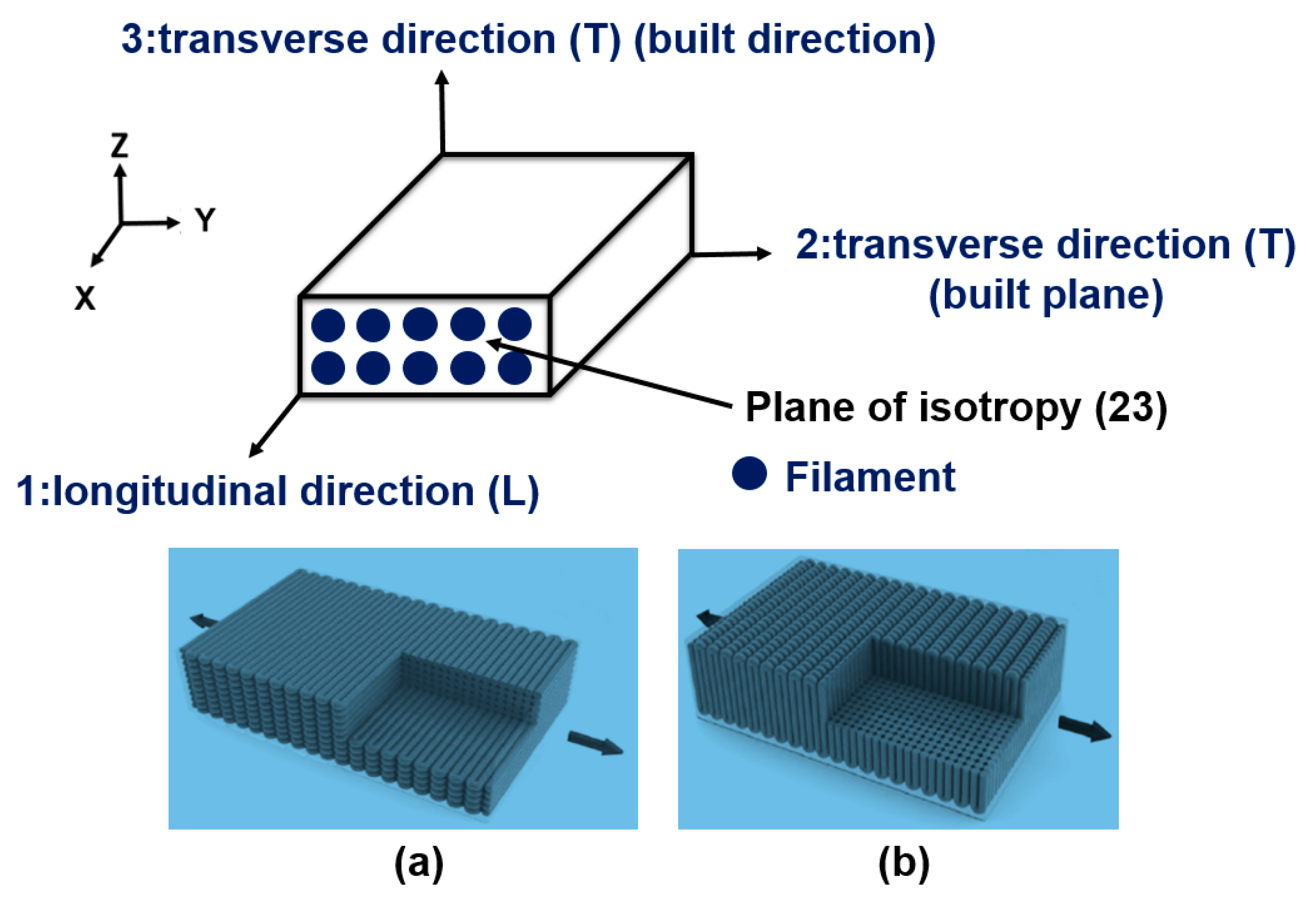
2.1. Local References Assignment in Mesh Elements

The purpose is to reproduce the printing trajectories inside a finite element model. The finite element code ABAQUS is used in this study. From the CAD file representing the part, the geometry is generated. Then an adaptive mesh is generated using an eight-node brick element with reduced integration C3D8R (i.e., one integration point per element). The use of C3D8R elements is motivated by the need to reproduce the layer by layer built in the model. This choice allows a simplification of the problem. The elements heights are fixed and must be equal to the layer thickness in order to ensure the reproduction of the built trajectories in a layer by layer process and facilitate the localization of elements in a certain layer (see Figure 2).
The procedure starts by treating the G-code and defining the trajectories that only correspond to the real material deposition. This means that the trajectories where the extrusion nozzle is off are eliminated. Assigning the material’s references goes through associating the material deposition trajectory with the elements of the numerical model. In each element, the vector tangent to a representative trajectory that intercepts the element faces is identified. This step requires distinguishing several cases according to the configuration of interception between the deposition trajectories and the element faces. Figure 3 demonstrates the possible cases. (i) If numerous trajectories belong to the element, the nearest to its Gauss’s point is chosen. (ii) If a discontinuity between the two trajectories is the closest to its Gauss’s point, the first trajectory analyzed is chosen with respect to the printing history. (iii) In the case where no trajectory intercepts the elements, the closest deposition trajectories are again selected.
The representative trajectory selected previously is considered as the first vector of the local reference. The third vector is always the same since it is the built direction (Z) perpendicular to the building plate (XY). A complete coordinate system is defined in each element by computing the cross-product of the first and the third vectors already known. This method was successfully applied on a compact tension CT specimen where complex trajectories were reproduced inside a finite element model after assigning the adequate materials’ references [24].

2.2. Mechanical Behavior Definition

After assigning local references inside the mesh elements, a mechanical behavior must be defined at the integration points. An orthotropic behavior is commonly used to model the mechanical behavior of FFF parts in the elastic domain. For the sake of simplification, both directions 2 and 3 defined in Figure 4 are considered equivalent since the built-in of both orientations have similar deposition patterns and weld lines structure. A transverse isotropic is therefore chosen. It requires the identification of five independent elastic constants; (i) E L : The Young’s modulus in the longitudinal direction of the filament, (ii) E T : The Young’s modulus in the transverse direction of the filament, (iii) ν L T : the in-plane Poisson’s ratio, (iv) ν T T : the out of the plane Poisson’s ratio, and (v) G L T : the in-plane shear modulus. Tensile tests with digital image correlation (DIC) are used to identify them. Thus, three orientations for the tensile specimens were chosen 0°, 90°, and 45°. The tensile specimens must be printed using the exact same printing parameters as the studied pre-structured material. This will ensure the reproduction of the mesostructure of the pre-structured material. As described previously, the authors decided to approach the material as homogenous. This means that the air gap portion is not subtracted from the geometrical cross-section. Therefore, the effect of the air gap volume fraction is directly incorporated in the identified material’s constants.

3. Experimental Setups

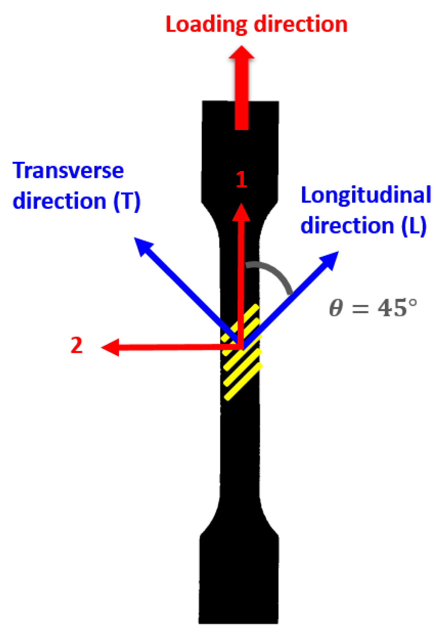
3.1. Fabrication of the Specimen

The specimens were designed according to the ASTM D638-03 norm “Standard Test Method for Tensile Properties of Plastics” [26]. The fused deposition modeling fabrication process was conducted on a Makerbot replicator ×2 with a flat printing configuration. The filament is made of white ABS (Acrylonitrile Butadiene Styrene) material so that a better contrast can be achieved while performing the DIC analysis. The printing parameters described in Table 1 are the same for all the specimens studied in this paper.
The slicing software Slic3r [27] was used to generate the G codes. This software was chosen since it allows a unique infill angle for all layers via the modifier feature. Three infill angles are used 0° representing the longitudinal direction of the filament, 90° for the transverse direction of the filament, and a 45° angle to study the shear behavior. Six specimens were fabricated for each orientation.

3.2. Tensile Tests with Digital Image Correlation

The tensile test machine Instron 4411 was used to perform the tensile tests. The loading rate was fixed at 1 mm/min. A camera with a resolution of 1280 pixels × 960 pixels was used to record a snapshot every 0.6 s while performing the test. This frequency gives an accurate reproduction of the tensile curves. The speckle was applied manually through a black paint spray. After collecting the snapshots, the DIC software NCORR [28] allows a quantitative analysis of the strain. It tracks the displacement of the speckles on each snapshot during the loading phase and uses it to interpret the kinematic field maps on a specific region of interest (ROI). A subset size of 15 pixels and a spacing of 2 pixels were used for data treatment. The images were treated as described in [29]. The method uses specific dummy sensors placed next to the jaw’s location in order to calculate the true value of displacement.

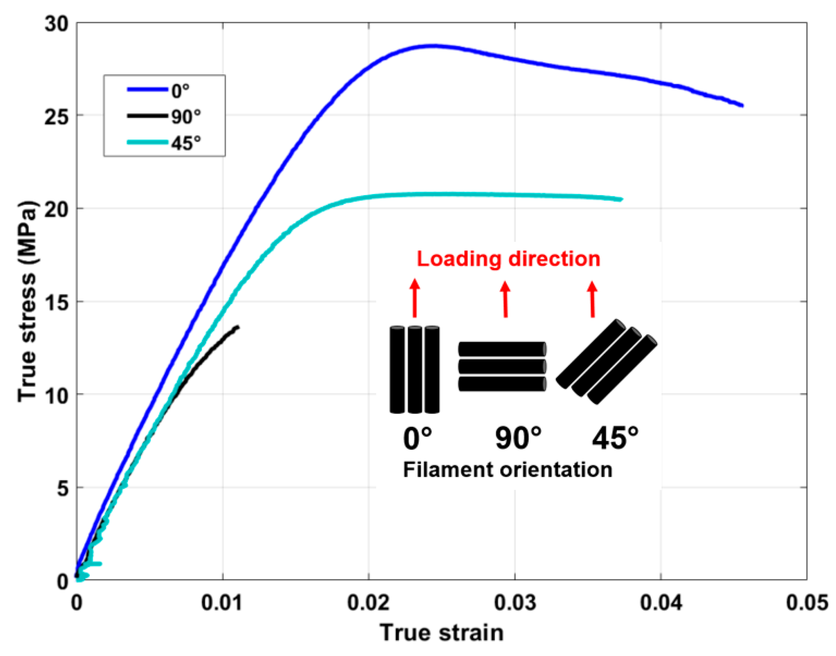
3.3. Tensile Tests Results

For every performed tensile test, the calculated Young’s modulus value will indirectly take into account the existing air gap by computing the engineering stress via the geometrical section. The calculations are made with respect to the D638 ASTM norm [26]: Young’s modulus is calculated as the slope of the tangent to the true stress-strain curve at low stress. To get such a curve, the assumption of volume conservation was made since the volume variation data is not available. The DIC analysis gives an estimation of the average value of the transversal and the longitudinal strain, which are used to calculate the Poisson’s ratio values. The yield strength is calculated via the 0.2% strain offset method. The results are displayed in Table 2.
The experimental tensile curves show that the material exhibits different behaviors according to the filament orientation (see Figure 5). For the 90° orientation, the elongation at break is almost equal to the elongation at yield strength. Thus, the behavior can be assumed perfectly elastic with a brittle fracture. On the other hand, the 0° specimens display the highest tensile strength of 23.54 MPa since the loading is directly applied on the longitudinal direction of the filament considered as the strongest direction. Here the behavior has a pronounced plastic behavior directly linked to a ductile fracture. In addition, a softening was observed in this direction. This softening behavior can be explained by referring to the work of Dundar et al. [30]. In fact, ABS material exhibits a strain-softening behavior at a low strain rate, which was around 10−4 s−1 for the tensile tests. Finally, the 45° specimen displays an intermediary behavior between both 0° and 90° with an almost elastic perfectly plastic behavior. The yield strength is found equal to 17.53 MPa. The fracture is also ductile and occurs at a 45° angle at the welding line direction.
These findings are coherent with the work of Alaimo et al. [31] which showcased the same behavior for the studied orientations. Young’s modulus is slightly lower but this can be explained by the difference in the extrusion temperature. The extrusion temperature used to fabricate the specimen is 235 °C while the temperature of extrusion used by Alaimo was around 255 °C. A higher extrusion temperature enhances the bonding between the filament and thus, the mechanical stiffness increases [32]. For the Poisson’s ratio of the 0° oriented sample, the same value was found by Rodriguez et al. [33]. For the yield strength, Alaimo [31] found a yield strength equal to 26.3 MPa, 14.6 MPa, and 18.54 MPa while the authors found 23.54 MPa, 13.3 MPa, and 17.53 MPa for 0°, 90°, and 45° respectively. It should be noted that all comparisons with the bibliographic references must be done with a similar printing configuration to avoid any perturbation from one of the printing parameters.
Conclusively, the material exhibits an overall quasi-isotropic stiffness. The difference between the 0° Young’s modulus and the 90° Young’s modulus does not exceed 16%. This means that welding lines are not affecting the material stiffness in the elastic domain. The anisotropy was mainly observed at the yielding and fracture points. Therefore, it was decided to employ an anisotropic yielding criterion to model the transition between elastic and plastic domains.

4. Implementation of the Pre-Structured Material Behavior

4.1. Transverse Isotropic Law Identification

As described previously, a transverse isotropic law is chosen to model the 3D printed material behavior. Thus, five independent elastic constants must be identified. Both Young’s modulus E L and E T and the in-plane Poisson’s ratio ν L T are directly identified from the tensile test results. The longitudinal Young’s modulus and the in-plane Poisson’s ratio are the ones calculated on the 0° specimen. The transverse Young’s modulus is the one calculated with the 90° specimen.

4.1.1. The In-Plane Shear Modulus G L T

By establishing the relationship between the global reference and the local reference defined in Figure 6, where the plane stress assumption is presumed, Young’s modulus in the loading direction (global reference 1) can be expressed as a function of the transverse isotropic elastic constants and the printing angle. The same relation (see Equation (1)) [34] is used to study the stress analysis of fiber-reinforced composite materials.
E 1 = E L cos 4 θ + ( E L G L T 2 ν L T ) sin 2 θ cos 2 θ + E L E T sin 4 θ
where:
  • θ : Printing angle
  • E L : Young’s modulus in the longitudinal direction
  • E T : Young’s modulus in the transverse direction
  • ν L T : The in-plane Poisson’s ratio
  • G L T : The in-plane shear modulus
  • E 1 : Young’s modulus in the loading direction (global reference)
By using the 45° specimen, the following equation is deducted:
G L T = ( 4 E 45 ° 1 E L 1 E T + 2 ν L T E L ) 1
where: E 45 ° is the experimental Young’s modulus from the 45° specimen. A value of 545 MPa of the in-plane shear modulus was calculated. A higher value was given by Alaimo et al. [31] equal to 641 MPa, which was already explained by the difference of the extrusion temperature.

4.1.2. The Out-of-Plane Poison’s Ratio ν T T

The compliance matrix C _ _   1 of the transverse isotropic material shows that the out- of-plane Poisson’s ratio ν T T is not activated in the case of the plane stress assumption unless the out-of-plane displacement is calculated. However, the DIC analysis employed here provides only the displacement field in 2D ROI. Therefore, the out-of-plane Poisson’s ratio ν T T cannot be identified using the available data. Otherwise, it was proven that its value would not influence the 2D material behavior because it only affects the out-of-plane strain component. For the developed model, ν T T was taken as the average value between ν T L and ν L T   . A value of ν T T = 0.3416 will be employed.

4.1.3. Stiffness Matrix C _ _

The transverse isotropic behavior is implemented in ABAQUS by computing all the components of the stiffness matrix C _ _ as shown by Equation (3).
C _ _ = ( 2592.3 1229.5 1229.5 1229.5 2184.1 1130.1 1229.5 1130.1 2184.1 0 0 545 545 527 )
This stiffness matrix C _ _ is defined at each C3D8R element with respect to the local reference defined in its integration point. This allows a local description of the material behavior based on the deposition trajectories at each point of the structure.

4.2. Anisotropic Yielding Criterion: Hill Criterion

The anisotropy was mainly observed at the yielding point. Indeed the 0° sample has the highest yield strength while the 90° sample has the lowest one. Where an anisotropic yielding criterion must be used, Hill’s criterion is used for this type of problem. It generalizes the Von Mises criterion by introducing anisotropy coefficients [35]. It has been used to describe the elastoplastic behavior of composites reinforced with short carbon fibers from 3D printing [36]. Likewise, it was efficient in underlining the anisotropy of the tensile strength of parts printed in PLA material.
The material has four different yield strengths according to the loading state, as described in Table 3, which must be identified to implement the Hill criterion. σ L 0 is the yield strength obtained from the 0° tensile tests and σ T 0 is obtained from the 90° tensile tests. They are equal to 23.54 MPa and 13.3 MPa respectively. The in-plane shear yield strength σ L T 0 is calculated by applying the laminate theory on the 45° specimen. The stress analysis described in Figure 6 is utilized. The tensile stress in the loading direction (global reference) is related to the stress components in the local reference and the printing angle through Equation (4).
σ 11 ( θ ) = [ cos 4 θ σ L 2 + sin 4 θ σ T 2 cos 2 θ sin 2 θ σ L 2 + cos 2 θ sin 2 θ σ L T 2 ] 1 2
where
  • σ 11 ( θ ): The tensile strength in loading direction (global reference)
  • θ : Printing angle
    σ L : The stress in the longitudinal direction of the filament
  • σ T : The stress in the transversal direction
  • σ L T : The in-plane shear stress
To access the in-plane shear yield strength, results from the 45° specimen are used. The following relation (see Equation (5)) is then established by taking θ = 45° and replacing σ 11 ( θ ) by the experimental yield strength of the 45°spceicmen.
σ L T 0 = ( 4 σ 45 ° 2 1 σ T 2 ) 1 2
A value of 11.65 MPa was found similar to the value found by [31] 12 ±   0.7 MPa.
For the out-of-plane shear yield strength, the torsion test is commonly used to identify its value. The experimental results reported in [37] by Balderrama-Armendariz et al. show that the out-of-plane shear yield is about 25 MPa. However, this value cannot be utilized herein since the printing parameters are substantially different. Therefore, both in-plane and out-of-plane shear yield strengths were assumed equal ( σ T T 0 = σ L T 0 ) .
The Hill criterion was implemented in ABAQUS software using the user-defined Hill’s potential function in ABAQUS [38]. It implies the definition of six different anisotropic yield stress ratios. As σ T T 0 = σ L T 0 , three independent ratios must be introduced as inputs. Those ratios (see Table 4) are expressed using a reference tensile yield stress σ 0 , which was chosen as the tensile yield strength in the longitudinal direction σ L 0 , and a reference shear yield stress τ 0 where τ 0 = σ 0 3 .

4.3. Plastic Flow Curve of the Filament (0° Specimen)

In order to study the material behavior in the plastic domain, it was decided to couple the Hill criterion with the curve flow for the 0° orientation. For the 0° specimen as shown in Figure 5, when the stress is below the yield stress, the material behaves elastically. After the yielding point, an isotropic hardening is observed and will be modeled via an exponential law defined by Equation (6) where: σ L 0 is the yield stress and ε p is the plastic strain and σ l i m i t is the hardening limit for the material and m is a positive dimensionless exponent.
σ = σ L 0 + σ l i m i t ( 1 e m ε p )
Using the experimental data, a least-square fit was used to identify those constants (see Table 5).
This model is only valid until reaching the tensile strength. The observed softening was discarded for the sake of simplicity. A stress saturation is assumed up to the fracture point with only an increase of the plastic strain. This model was implemented in ABAQUS using a tabular law that describes the evolution of the plastic strain from the yielding point up to the breaking point.

5. Results and Discussions

All the simulations in this study were carried out using ABAQUS implicit solver. A quasi-static time-independent loading step is defined to model the various tests with an applied displacement as a loading condition. All models utilized C3D8R mesh elements with adequate mesh sizes according to the geometry and the deposition trajectories requirement. The implementation of the mechanical behavior as defined in the previous section is used for all simulations.

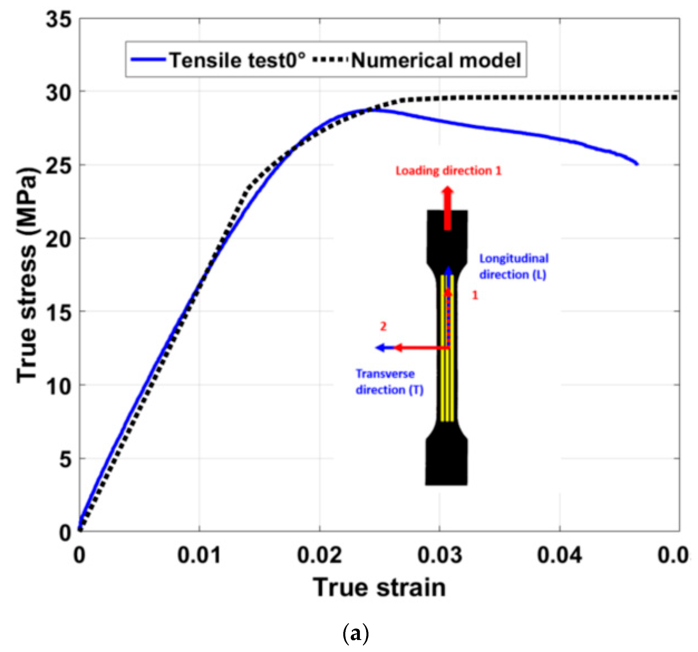
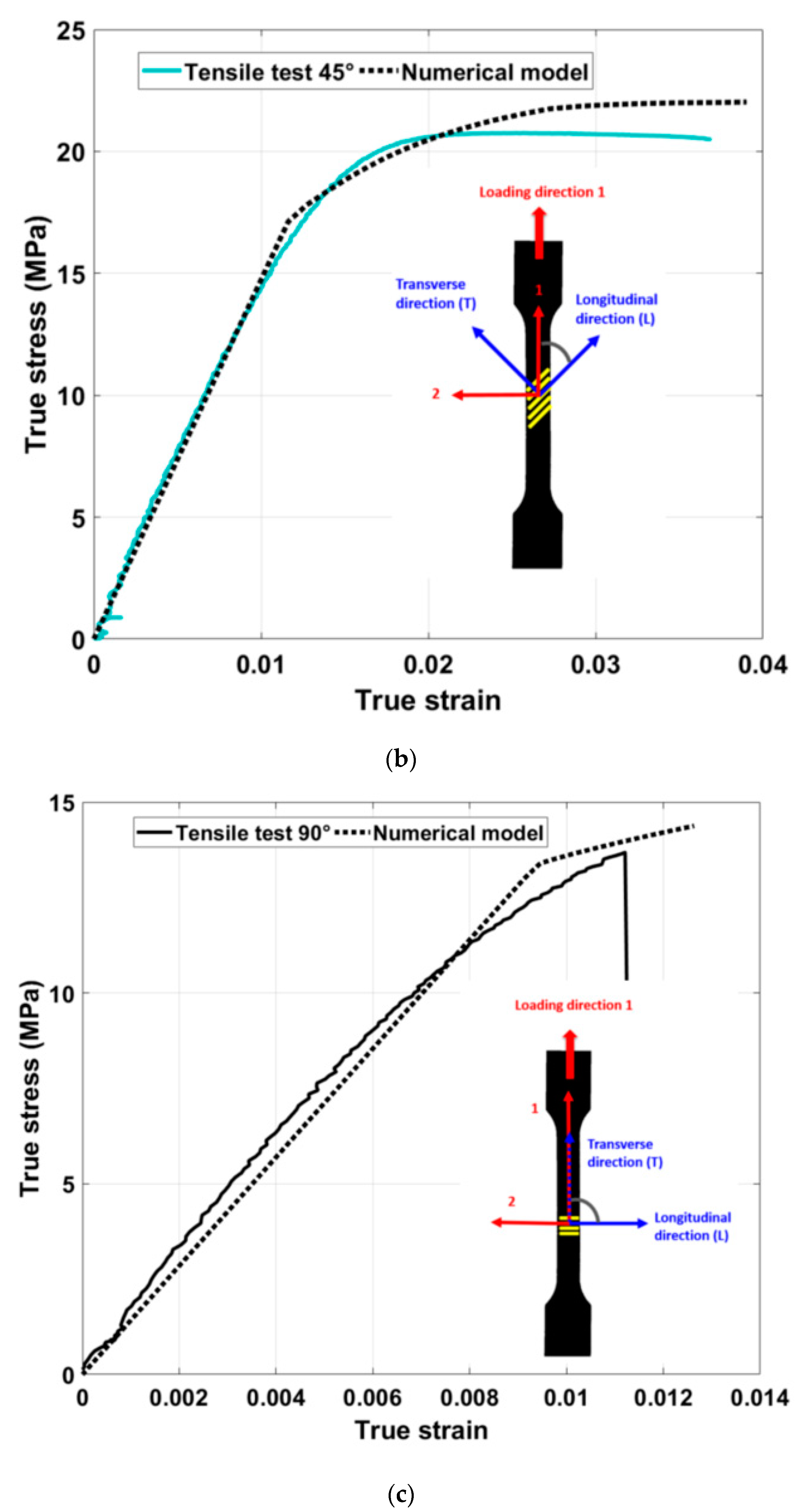
5.1. Tensile Tests Prediction

The finite element model for the tensile specimen geometry was created in ABAQUS software. Three models were later defined by assigning local material references with respect to the printing trajectories. Three different simulations have been carried out to simulate the behavior of each of the specimens according to the suggested model. The part of the specimen pinched between the fixed jaws is encastered and a displacement is applied on a reference point coupled with the part pinched between the mobile jaws.
Figure 7 compares the stress-strain curves obtained experimentally with those obtained by finite element simulations. The results show that for all three cases, the elastic behavior is well reproduced with a slight difference because of the simplifications described before. Thus, the model predicts well the stress evolution until the yielding point. By comparing the model response for the three different orientations, it is clear that the anisotropic yielding criterion taken in the model captures the yield point in the experimental curves. The transition between the elastic and the plastic domain for the 0° specimen occurs around the value of σ L 0 . In addition, for this orientation, the saturation of the stress at the average tensile strength is noticed (see Figure 7a). The onset of plastic behavior observed for the 45° tensile sample is well simulated (see Figure 7b) by coupling Hill’s criterion with the 0° flow curve. Therefore, the numerical approach is able to highlight the anisotropic strengths according to the filament orientation. For the sample with 90° (Figure 7c), orientation exhibits a brittle fracture. However, a plastic behavior appears in the numerical response. This behavior was intentionally discarded since it does not appear in the experimental tests. The elongation at fracture was managed by applying the appropriate corresponding displacement value without implementing a fracture initiation criterion. The average values reported in Table 2 of the fracture elongation were respected.
The model allows good prediction of the elastic domain without any estimation of the air gap. The plastic component was defined in order to demonstrate the ability of Hill’s criterion to predict the anisotropy with the material yield strength. By only implementing the plastic flow curve for the 0° orientation, it has been shown that it is possible to predict the mechanical response of the material in different orientations.

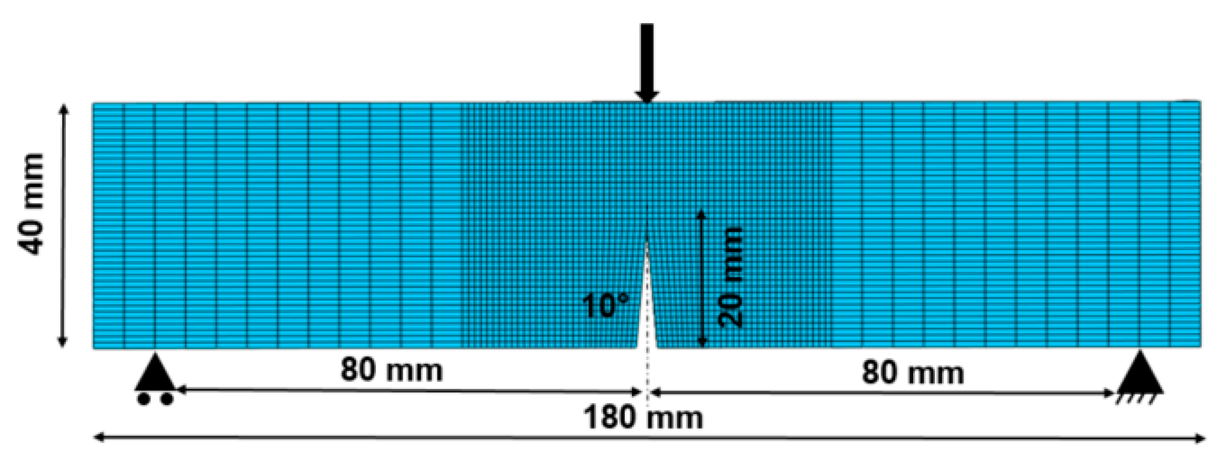
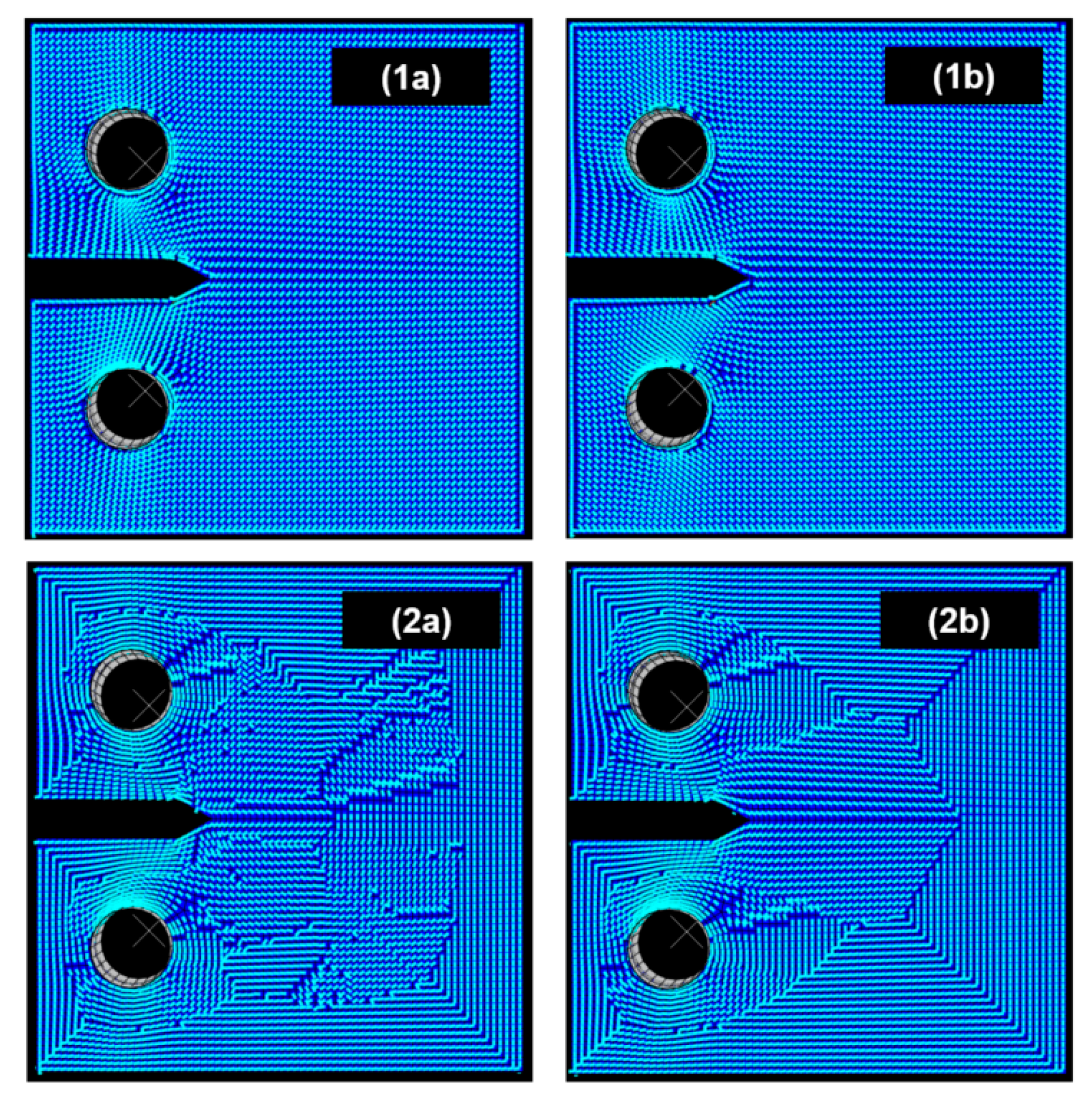
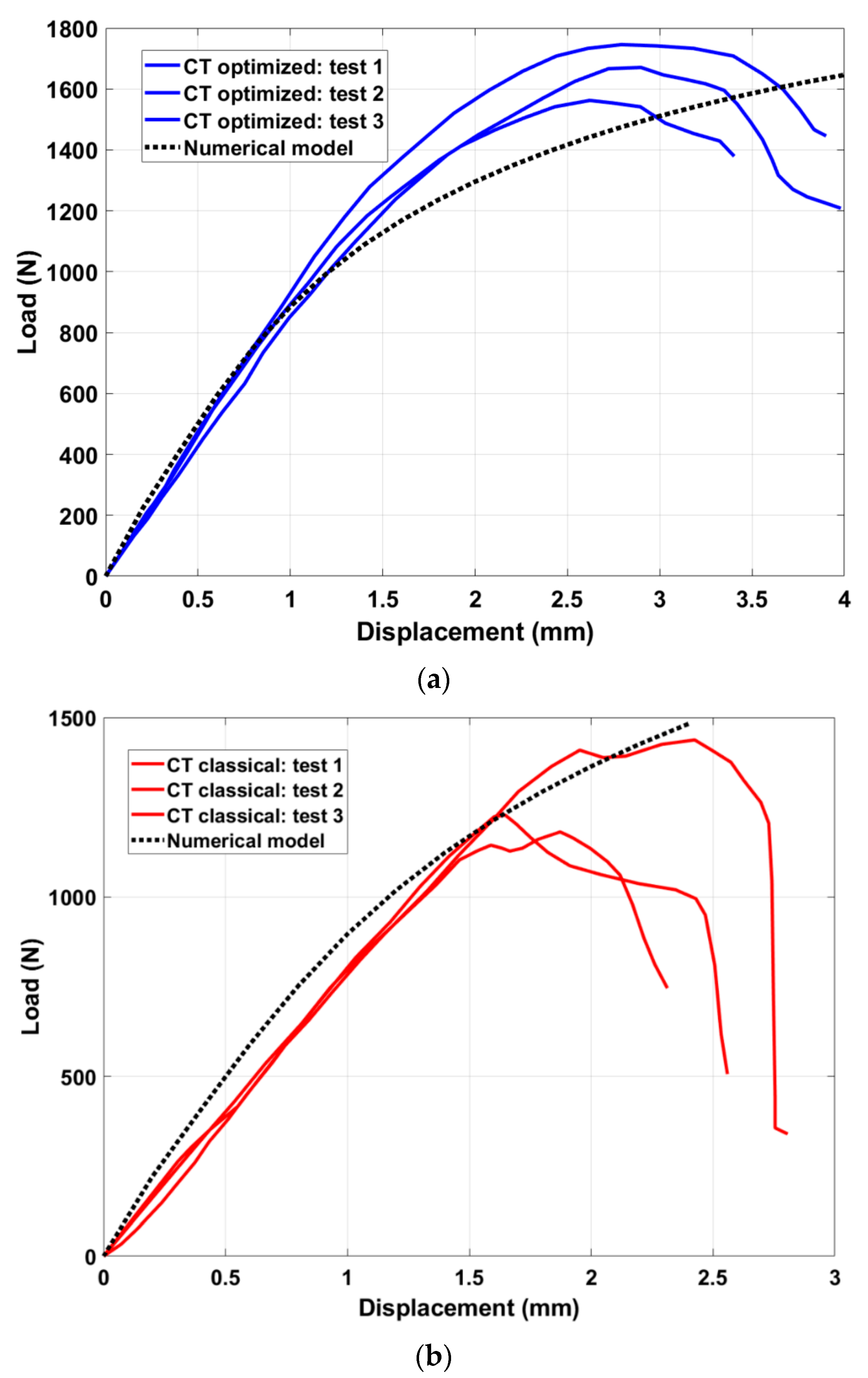
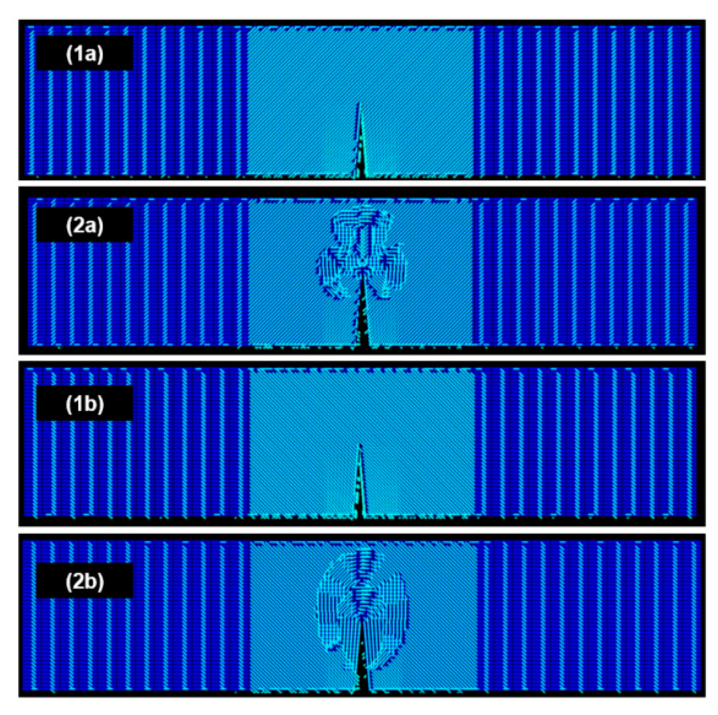
5.2. Compact-Tension Specimen
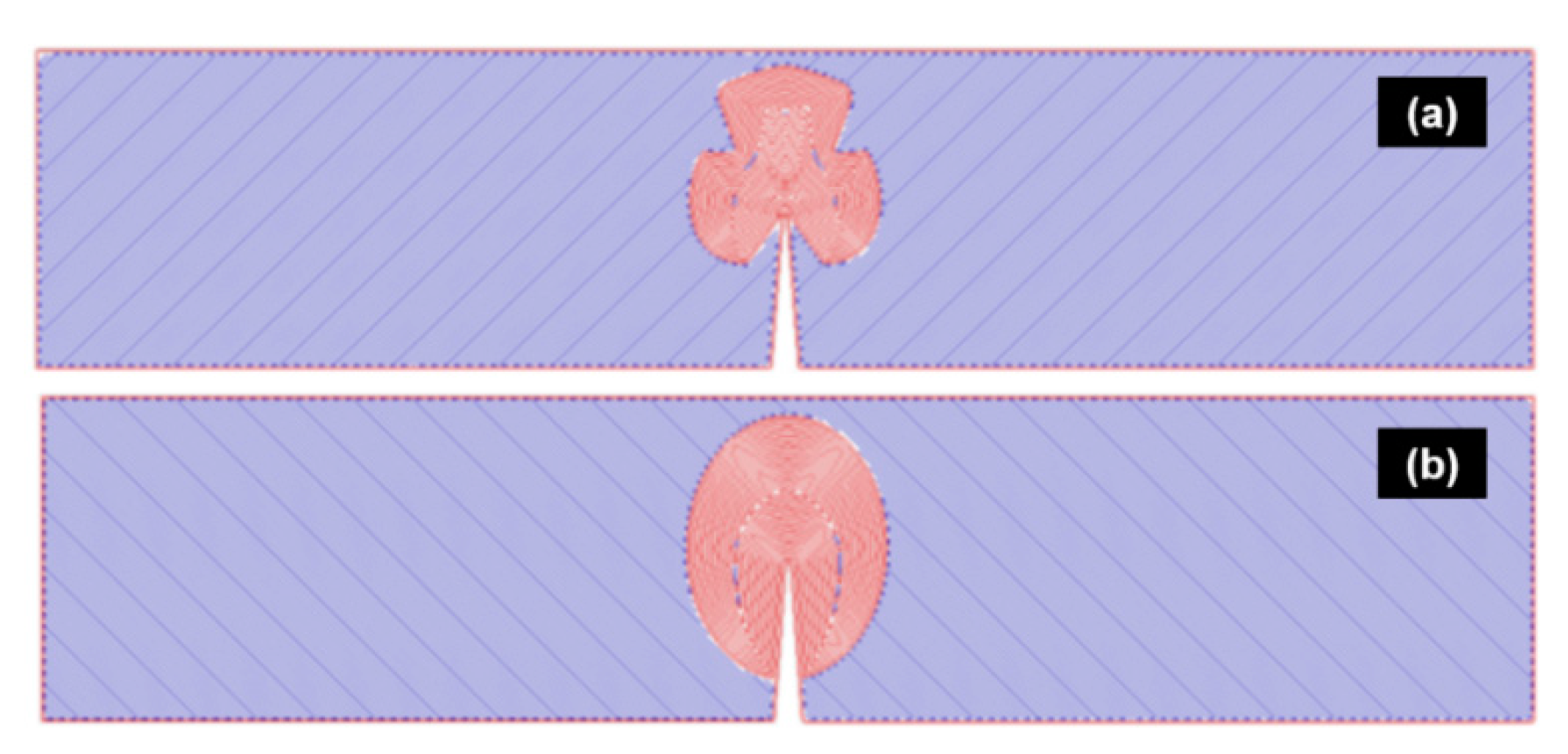
In this section, the model’s ability to predict the global response of a compact tension CT specimen, defined in [6], will be checked. After treating both the classical and the optimized G codes of the corresponding geometries, two finite element models were created. The numerical model definition with the boundary conditions is described in [24]. The part is sliced along the Z direction to match the layers from the G code. The local material’s references are assigned for both kinds of samples. Figure 8 shows the vectors that correspond to the deposition trajectory in each element. For the optimized specimen, since two principal directions were reproduced, only two material’s references definition per layer can be observed. The model’s responses will be compared with the experimental data collected from the work of Gardan et al. [6]. The boundaries conditions defined in [24] are maintained the same for this study. Two rigid bodies are used. One to model the fixed pin and the other represents the mobile one.
Figure 9 compares both experimental and numerical results. The drop of the stress observed in the experimental curves results from the crack initiation and growth from the notch tip. Therefore, the simulation cannot reproduce this behavior because the material damage and fracture are not taken into account by the model. Regarding the linear behavior of the samples, the model gives a good prediction of the stiffness for the optimized specimen and slightly overestimates it for the classical one. For the optimized specimen, where a ductile-like curve is obtained by the test, the model underestimates the load values (see Figure 9a). This is mainly related to a numerical plastic behavior along the transversal direction that is not omitted in the model.

5.3. Beam Specimen

The work reported in Lanzilotti et al. [7] focused on applying the optimized deposition method on the Single Edge Notched Bending SENB specimen. It reproduces the principal stress direction in the V notch tip vicinity and keeps a classical deposition ± 45° elsewhere. The printing trajectories from the G code are shown in Figure 10.
The SENB specimen dimensions and the boundary conditions used for the simulations are shown in Figure 11. A mesh size of 0.56 mm was used in the V notch area to better capture the deposition trajectories. This value is equal to the thread width used during the printing. A bigger mesh size can still capture the trajectories elsewhere since they have unidirectional orientations. This will also allow a reduction in computational time. The first vectors representing the deposition trajectories of all the local references are showcased in all the integration points in Figure 12.
Interestingly, the numerical response seems to be practically the same for both models (classical and optimized). The mesh elements’ orientations have almost no effect on the global numerical response. A numerical stiffness equal to 253.15 N/mm was calculated for both models. Although, the classical specimen has an average stiffness of 174.3 ± 11.8 N/mm, the stiffness of the optimized sample is 224.3 ± 12.7 N/mm. This is related to the quasi-isotropic stiffness of the material since no large difference in the elastic modulus was found between the longitudinal and the transversal directions (16%). Moreover, the modification of the raster orientation is only carried out locally in the notch tip vicinity. The remaining domain is built by ± 45° stacked layers. Although this local modification leads to the improvement of the sample fracture toughness, however, no substantial difference was found in the elastic response of the model. The model assumes the material continuum. This assumption omits any potential effect of the air gaps, weld lines, and even the anisotropy of the filament itself. This partially interprets the difference found between the sample stiffness measured experimentally and numerically. On the other hand, the simulation results show that the influence of the local modification of filament orientation in the notch tip vicinity is vanishingly small so that the model cannot capture it.
The model uses a stiffness matrix and materials constants from tensile tests printed so that the filaments are stacked in the same direction. This is supposed to maximize the bonding conditions between layers, and can therefore explain why the model overestimates the experimental stiffness. The biggest area of the specimen is printed using stacking layers at ± 45°. A 90° crossing angle between filaments in two different layers would accordingly decrease the bonding conditions.

6. Conclusions

A simplified numerical model to predict the mechanical behavior of FFF 3D printing parts has been proposed. The model tackles successfully the anisotropic built configuration by assigning local material references in mesh elements. It approaches the material as homogenous and uses specific materials constants to introduce the anisotropy related to complex deposition trajectories. The present findings confirm that the material has a quasi-isotropic elastic behavior since both longitudinal and transversal Young’s modulus are roughly equal. Hill’s criterion coupled with the plastic flow curve of the filament has been used to identify the strength anisotropy in tensile specimens with different raster angles. The longitudinal direction has the highest yield strength and a ductile behavior while the transversal one is the weakest and exhibits a fragile behavior at the yielding point.
The model is not able to capture the behavior where the optimized deposition method is applied to a small zone compared to the area of the specimen. Future work could fruitfully explore this issue further by taking into account the bonding conditions between the filaments. Axiomatically the model can be upgraded by assigning local materials’ properties according to local bonding conditions.
Despite its limitations in reproducing local phenomena, the model is a key component in future attempts to understand the relation between the local deposition orientation and the material performance. The possibility of utilizing this model in the simulation of the mechanical behavior of 3D printed parts by FDM warrants further investigation and development. Finally, the model can be enriched with another simulation method (e.g., continuum damage mechanics or extended finite elements) in order to study the fracture behavior after crack initiation.

Author Contributions

Conceptualization, C.L.; Data curation, M.Z. and J.G.; Formal analysis, A.M. and N.R.; Funding acquisition, M.Z.; Investigation, M.Z., J.G., P.L. and A.M.; Methodology, J.G., P.L., A.M. and C.L.; Project administration, J.G. and P.L.; Software, M.Z. and A.M.; Supervision, J.G. and P.L.; Validation, N.R.; Writing—original draft, M.Z.; Writing—review & editing, J.G., P.L., A.M. and N.R. All authors have read and agreed to the published version of the manuscript.

Funding

This research was funded by the French Government, the European Regional Development Fund (ERDF), University of Technology of Troyes (UTT) and EPF Engineering School.

Institutional Review Board Statement

Not applicable.

Informed Consent Statement

Not applicable.

Data Availability Statement

Not applicable.

Acknowledgments

The authors gratefully acknowledge the French Government, the European Regional Development Fund (ERDF), University of Technology of Troyes (UTT) and EPF Engineering School for their financial support.

Conflicts of Interest

The authors declare that they have no known competing financial interests or personal relationships that could have appeared to influence the work reported in this paper.

References

  1. Gardan, J. Smart materials in additive manufacturing: State of the art and trends. Virtual Phys. Prototyp. 2019, 14, 1–18. [Google Scholar] [CrossRef]
  2. Li, J.; Yang, S.; Li, D.; Chalivendra, V. Numerical and experimental studies of additively manufactured polymers for enhanced fracture properties. Eng. Fract. Mech. 2018, 204, 557–569. [Google Scholar] [CrossRef]
  3. Madugula, S.; Giraud-Moreau, L. Renforcement de la structure interne de pièces imprimées par une technique de remaillage adaptée à l’extrusion en continu. In Proceedings of the CSMA 2019, Giens, France, 13–17 May 2019; p. 9. [Google Scholar]
  4. Gardan, J.; Makke, A.; Recho, N. A Method to Improve the Fracture Toughness Using 3D Printing by Extrusion Deposition. Procedia Struct. Integr. 2016, 2, 144–151. [Google Scholar] [CrossRef] [Green Version]
  5. Gardan, J.; Makke, A.; Recho, N. Fracture Improvement by Reinforcing the Structure of Acrylonitrile Butadiene Styrene Parts Manufactured by Fused Deposition Modeling. 3D Print. Addit. Manuf. 2019, 6, 113–117. [Google Scholar] [CrossRef]
  6. Gardan, J.; Makke, A.; Recho, N. Improving the fracture toughness of 3D printed thermoplastic polymers by fused dep-osition modeling. Int. J. Fract. 2018, 210, 1–15. [Google Scholar] [CrossRef]
  7. Lanzillotti, P.; Gardan, J.; Makke, A.; Recho, N. Enhancement of fracture toughness under mixed mode loading of ABS specimens produced by 3D printing. Rapid Prototyp. J. 2019, 25, 679–689. [Google Scholar] [CrossRef]
  8. Kim, J.; Kang, B.S. Optimization of Design Process of Fused Filament Fabrication (FFF) 3D Printing. In Volume 2: Advanced Manufacturing; American Society of Mechanical Engineers: Pittsburgh, PA, USA, 2018; p. V002T02A060. [Google Scholar]
  9. Ahn, S.; Montero, M.; Odell, D.; Roundy, S.; Wright, P.K. Anisotropic material properties of fused deposition modeling ABS. Rapid Prototyp. J. 2002, 8, 248–257. [Google Scholar] [CrossRef] [Green Version]
  10. Rankouhi, B.; Javadpour, S.; Delfanian, F.; Letcher, T. Failure Analysis and Mechanical Characterization of 3D Printed ABS with Respect to Layer Thickness and Orientation. J. Fail. Anal. Prev. 2016, 16, 467–481. [Google Scholar] [CrossRef]
  11. Xu, L.R.; Leguillon, D. Dual-Notch Void Model to Explain the Anisotropic Strengths of 3D Printed Polymers. J. Eng. Mater. Technol. 2019, 142. [Google Scholar] [CrossRef]
  12. Allum, J.; Moetazedian, A.; Gleadall, A.; Silberschmidt, V.V. Interlayer bonding has bulk-material strength in extrusion additive manufacturing: New understanding of anisotropy. Addit. Manuf. 2020, 34, 101297. [Google Scholar] [CrossRef]
  13. Tymrak, B.M.; Kreiger, M.; Pearce, J.M. Mechanical properties of components fabricated with open-source 3-D printers under realistic environmental conditions. Mater. Des. 2014, 58, 242–246. [Google Scholar] [CrossRef] [Green Version]
  14. Riddick, J.C.; Haile, M.A.; Von Wahlde, R.; Cole, D.P.; Bamiduro, O.; Johnson, T.E. Fractographic analysis of tensile failure of acrylonitrile-butadiene-styrene fabricated by fused deposition modeling. Addit. Manuf. 2016, 11, 49–59. [Google Scholar] [CrossRef]
  15. Ahn, S.H.; Baek, C.; Lee, S.; Ahn, I.S. Anisotropic Tensile Failure Model of Rapid Prototyping Parts—Fused Deposition Modeling (FDM). Int. J. Mod. Phys. B 2003, 17, 1510–1516. [Google Scholar] [CrossRef]
  16. Croccolo, D.; De Agostinis, M.; Olmi, G. Experimental characterization and analytical modelling of the mechanical be-haviour of fused deposition processed parts made of ABS-M30. Comput. Mater. Sci. 2013, 79, 506–518. [Google Scholar] [CrossRef]
  17. Cantrell, J.T.; Rohde, S.; Damiani, D.; Gurnani, R.; DiSandro, L.; Anton, J.; Young, A.; Jerez, A.; Steinbach, D.; Kroese, C.; et al. Experimental characterization of the mechanical properties of 3D-printed ABS and polycarbonate parts. Rapid Prototyp. J. 2017, 23, 811–824. [Google Scholar] [CrossRef]
  18. Rohde, S.; Cantrell, J.; Jerez, A.; Kroese, C.; Damiani, D.; Gurnani, R.; DiSandro, L.; Anton, J.; Young, A.; Steinbach, D.; et al. Experimental Characterization of the Shear Properties of 3D–Printed ABS and Polycarbonate Parts. Exp. Mech. 2018, 58, 871–884. [Google Scholar] [CrossRef]
  19. Casavola, C.; Cazzato, A.; Moramarco, V.; Pappalettere, C. Orthotropic mechanical properties of fused deposition mod-elling parts described by classical laminate theory. Mater. Des. 2016, 90, 453–458. [Google Scholar] [CrossRef]
  20. Biswas, P.; Guessasma, S.; Li, J. Numerical prediction of orthotropic elastic properties of 3D-printed materials using mi-cro-CT and representative volume element. Acta Mech. 2020, 231, 503–516. [Google Scholar] [CrossRef]
  21. Nasirov, A.; Fidan, I. Prediction of mechanical properties of fused filament fabricated structures via asymptotic homog-enization. Mech. Mater. 2020, 145, 103372. [Google Scholar] [CrossRef]
  22. Ghandriz, R.; Hart, K.; Li, J. Extended finite element method (XFEM) modeling of fracture in additively manufactured polymers. Addit. Manuf. 2020, 31, 100945. [Google Scholar] [CrossRef]
  23. Zhao, Y.; Chen, Y.; Zhou, Y. Novel mechanical models of tensile strength and elastic property of FDM AM PLA materials: Experimental and theoretical analyses. Mater. Des. 2019, 181, 108089. [Google Scholar] [CrossRef]
  24. Zouaoui, M.; Labergere, C.; Gardan, J.; Makke, A.; Recho, N.; Alexandre, Q.; Lafon, P. Numerical Prediction of 3D Printed Specimens Based on a Strengthening Method of Fracture Toughness. Procedia CIRP 2019, 81, 40–44. [Google Scholar] [CrossRef]
  25. Cole, D.P.; Riddick, J.C.; Jaim, H.M.I.; Strawhecker, K.E.; Zander, N.E. Interfacial mechanical behavior of 3D printed ABS. J. Appl. Polym. Sci. 2016, 133. [Google Scholar] [CrossRef]
  26. D20 Committee. Test Method for Tensile Properties of Plastics; ASTM International: West Conshohocken, PA, USA, 2010. [Google Scholar]
  27. Slic3r Manual—Welcome to the Slic3r Manual. Available online: https://manual.slic3r.org/ (accessed on 24 June 2020).
  28. Blaber, J.; Adair, B.S.; Antoniou, A. Ncorr: Open-Source 2D Digital Image Correlation Matlab Software. Exp. Mech. 2015, 55, 1105–1122. [Google Scholar] [CrossRef]
  29. Zouaoui, M.; Gardan, J.; Lafon, P.; Labergere, C.; Makke, A.; Recho, N. Transverse Isotropic Behavior Identification using Digital Image Correlation of a Pre-structured Material Manufactured by 3D Printing. Procedia Struct. Integr. 2020, 28, 978–985. [Google Scholar] [CrossRef]
  30. Dundar, M.A.; Dhaliwal, G.S.; Ayorinde, E.; Al-Zubi, M. Tensile, compression, and flexural characteristics of acrylonitrile–butadiene–styrene at low strain rates: Experimental and numerical investigation. Polym. Polym. Compos. 2020, 0967391120916619. [Google Scholar] [CrossRef]
  31. Alaimo, G.; Marconi, S.; Costato, L.; Auricchio, F. Influence of meso-structure and chemical composition on FDM 3D-printed parts. Compos. Part B Eng. 2017, 113, 371–380. [Google Scholar] [CrossRef]
  32. Attolico, M.A.; Casavola, C.; Cazzato, A.; Moramarco, V.; Renna, G. Effect of extrusion temperature on fused filament fabrication parts orthotropic behaviour. Rapid Prototyp. J. 2019, 26, 639–647. [Google Scholar] [CrossRef]
  33. Rodríguez, J.F.; Thomas, J.P.; Renaud, J.E. Mechanical behavior of acrylonitrile butadiene styrene (ABS) fused deposition materials. Experimental investigation. Rapid Prototyp. J. 2001, 7, 148–158. [Google Scholar] [CrossRef]
  34. Hyer, M.W. Stress Analysis of Fiber-Reinforced Composite Materials; Updated edition; DEStech Publications: Lancaster, PA, USA, 2009. [Google Scholar]
  35. Hill, R. A theory of the yielding and plastic flow of anisotropic metals. Proc. R. Soc. Lond. A 1948, 193, 281–297. [Google Scholar]
  36. Bhandari, S.; Lopez-Anido, R.A.; Wang, L.; Gardner, D.J. Elasto-Plastic Finite Element Modeling of Short Carbon Fiber Reinforced 3D Printed Acrylonitrile Butadiene Styrene Composites. JOM 2020, 72, 475–484. [Google Scholar] [CrossRef]
  37. Balderrama-Armendariz, C.O.; Macdonald, E.; Espalin, D.; Cortes, D.; Wicker, R.; Maldonado-Macías, A. Torsion analysis of the anisotropic behavior of FDM technology. Int. J. Adv. Manuf. Technol. 2018, 96, 307–317. [Google Scholar] [CrossRef]
  38. Anisotropic Yield/Creep. Available online: https://abaqus-docs.mit.edu/2017/English/SIMACAEMATRefMap/simamat-c-anisoyield.htm (accessed on 15 September 2020).
Figure 1. Workflow of the modeling methodology.
Applsci 11 05075 g001
Figure 2. Correspondence between the layers heights (a) and the elements heights in ABAQUS mesh (b). Every layer from the G code contains different deposition trajectories.
Applsci 11 05075 g002
Figure 3. Possible interception cases between one mesh element C3D8R and the deposition trajectories.
Applsci 11 05075 g003
Figure 4. Transverse isotropic behavior for 3D printed parts; 1 is the longitudinal direction of the filaments, 2 is the transverse direction in the built plane illustrated in (a) and 3 is the second transverse direction that represents the built direction (b) [25].
Applsci 11 05075 g004
Figure 5. Tensile curves of three samples with different filament orientations (0°, 45°, and 90°).
Applsci 11 05075 g005
Figure 6. Local and global references definition for the 45° specimen.
Applsci 11 05075 g006
Figure 7. Model response of the tensile test specimens compared to a representative experimental curve. (a): 0° raster orientation and (b): 45° raster orientation and (c): 90° raster orientation.
Applsci 11 05075 g007aApplsci 11 05075 g007b
Figure 8. Numerical models of the CT specimen. (1) Corresponds to the classical deposition with ± 45 ° layers alternation. (2) For the optimized deposition; (a) denotes the first principal direction while (b) is for the second principal direction.
Applsci 11 05075 g008
Figure 9. Load-displacement curves of CT test. Numerical model response is compared to experimental results. (a) Classical samples are printed with ± 45° and (b) Optimized samples; the filament is oriented according to the principal direction of the stress.
Applsci 11 05075 g009
Figure 10. Deposition trajectories from the G code of the SENB specimen after applying the optimization method on the V notch vicinity. (a) First principal direction and (b) second principal direction.
Applsci 11 05075 g010
Figure 11. SENB specimen geometry’s definition and the boundary conditions for the numerical model.
Applsci 11 05075 g011
Figure 12. Numerical models of the SENB specimen. (1) Corresponds to the classical deposition with ± 45 ° layers alternation. (2) For the optimized deposition with principal stress reproduction in the V notch tip vicinity; (a) denotes the first principal direction while (b) is for the second principal direction.
Applsci 11 05075 g012
Table 1. Printing settings.
Printing ConfigurationBuilt Flat
Layer thickness0.25 mm (0.35 for the first one)
Extrusion temperature235 °C
Built plate temperature120 °C
Thread diameter1.7 mm
Infill density100%
MaterialABS (white)
Table 2. Results of tensile tests.
Orientation90°45°
MeanStd *MeanStdMeanStd
Young’s modulus (MPa)1680711414133148453
Offset yield strength 0.2% (MPa)23.541.5913.3 0.7817.530.95
Tensile strength (MPa)28.670.7913.860.6520.251.16
Elongation at fracture (%)4.901.311.120.183.650.46
Poisson’s ratio0.3710.0320.3120.0320.3420.028
* Std: standard deviation.
Table 3. Yield strengths designation for the transverse isotropic material.
Yield Strength DesignationLoading State on the Filaments
Tensile yield strength in the longitudinal direction: σ L 0 Applsci 11 05075 i001
Tensile yield strength in the transversal direction: σ T 0 Applsci 11 05075 i002
In-plane shear yield strength:   σ L T 0 Applsci 11 05075 i003
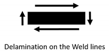
Out-of-plane shear yield strength: σ T T 0 Applsci 11 05075 i004
Table 4. Implementation of Hill’s potential function in ABAQUS using the yield stress ratios for the transverse isotropic material.
Ratio R L R T R L T = R L T
Expression σ L 0 σ 0 σ T 0 σ 0 σ L T 0   τ 0 = σ T T 0 τ 0
Value10.5650.857
Table 5. Exponential law fitting results.
σ l i m i t ( MPa ) m
Mean valueStdMean valueStd
6.583.41221.696.19
Publisher’s Note: MDPI stays neutral with regard to jurisdictional claims in published maps and institutional affiliations.

