SCCDNet: A Pixel-Level Crack Segmentation Network

Abstract

Cracks are one of the most serious defects that threaten the safety of bridges. In order to detect different forms of cracks in different collection environments quickly and accurately, we proposed a pixel-level crack segmentation network based on convolutional neural networks, which is called the Skip Connected Crack Detection Network (SCCDNet). The network is composed of three parts: the Encoder module with 13 convolutional layers pretrained in the VGG-16 network, the Decoder module with a densely connected structure, and the Skip-Squeeze-and-Excitation (SSE) module which connects the feature map shaving the same resolution in the Encoder and Decoder. We used depthwise separable convolution to improve the accuracy of crack segmentation while reducing the complexity of the model. In this paper, a dataset containing cracks collected in different scenes was established, and SCCDNet was trained and tested on this dataset. Compared with the advanced models, SCCDNet obtained the best crack segmentation performance, while F-score reached 0.7763.

1. Introduction

In modern society, the safety inspection of bridges is very important. Cracks are one of the most common defects of bridges. The timely detection and maintenance of cracks can effectively prevent the quality problems of the bridges from endangering human safety [1]. Due to the requirements for bridge safety, we need to successfully detect cracks and overcome the impact of noises on the bridge in real life which will influence the detection results, such as stains, scratches, and uneven illumination.

In recent years, crack detection algorithms based on computer vision have been continuously developed. Threshold segmentation [2], morphology [3], wavelet transform [4], and filter-based algorithms [5] have been applied to crack detection tasks. Although the above algorithms can achieve good detection accuracy after tuning the parameters, they can only be effective for images collected in a specific environment. Changes in illumination and shooting distance will reduce the detection accuracy, so they cannot meet actual engineering requirements. Li et al. [6] proposed a Neighboring Difference Histogram Method (NDHM) algorithm, which binarizes the images by calculating the global optimization threshold of the image. However, this algorithm is ineffective when there are a lot of stains and shadows in the image. Chun et al. [7] proposed a crack detection methodology based on pixel values and geometric shapes in two stages, which achieved an accuracy of 99.7% and on F-measure of 0.6952. The F* Seed-growing Approach (FoSA) [8] algorithm is proposed on the basis of the NDHM algorithm, which enhances its anti-noise ability; CrackTree [9] is an automatic crack detection algorithm that solves the influence of shadows similar to cracks on the detection results. Crack detection algorithms based on traditional computer vision generally focus on the understanding of local features and global features of the image. The parameters of the algorithms are mostly designed for specific datasets and crack patterns. When the scenes and features of the datasets change, the detection accuracy will always decrease. For instance, the FoSA algorithm and the CrackTree algorithm have good detection results for fine cracks, but the detection accuracy for thick cracks will decrease.

To overcome the limitations of traditional computer vision algorithms, the Convolutional Neural Networks (CNNs) are applied to vision tasks. CNNs were first proposed by LeCun et al. [10], which can yield abundant hierarchical features in the image, and then can better understand the objects in the image [11]. CNNs are widely used in many spheres such as image classification [12,13], object detection [14], semantic segmentation [15,16,17], and are gradually being applied to crack detection tasks.

In order to detect cracks timely, researchers design classifiers to determine whether image units belong to cracks. The network designed by Cha et al. [18] based on CNNs combined with sliding window technology can detect the crack images whose resolutions are greater than 256 × 256; the classifier designed by Zhang et al. [19] can detect crack images with a resolution of 3264 × 2448; Soukup et al. [20] used supervised learning to train CNNs classifiers and discussed the impact of regularization methods such as unsupervised hierarchical pre-training and training set expansion on the results. However, these image-level crack detection algorithms can only judge whether there are cracks in small image units and cannot accurately segment the cracks in pixel-level, so it is impossible for them to analyze the characteristics of cracks such as length and width. In addition to algorithms based on CNNs, Artificial Neural Networks (ANNs) [21,22,23,24] and Support Vector Machines (SVMs) [25,26] have been verified to be able to classify crack images, which have the same problems.

In some cases, we need to calculate the cracks’ length and width so that we could evaluate the safety of the targets. Therefore, we have to do pixel-level crack detection instead of path-level crack detection to achieve this target. This kind of pixel-level crack detection can be equivalent to semantic segmentation task. U-Net [27] is a common semantic segmentation network. It uses an Encoder-Decoder structure and the skip-connection strategy to concatenate the shallow feature maps with the deeper feature maps, which greatly improves the network performance, but at the same time, it will increase model parameters; SegNet [28] also uses the skip-connection strategy to introduce the maximum pooling parameter in the Encoder module into the Decoder module, greatly improving the computational efficiency of the model, but at the expense of detection accuracy. Yamane et al. [29] proposed a crack detection method based on the model of semantic segmentation, which could alleviate the influence of the trace of tie-rod holes and formworks on the detecting accuracy. CrackNet [11] was proposed in 2017 for pixel-level crack detection tasks. Different from the traditional CNNs structure, it removes the pooling layer to avoid the loss of details caused by excessive downsampling. Although CrackNet can achieve better crack detection accuracy, artificially designed filters limit the learning ability of the model. CrackNet-V [30] is improved on the basis of CrackNet. Its model has a deeper structure and fewer parameters and improves the efficiency of crack detection and calculation. However, the data set used by this algorithm only contains specific types of cracks, and it is difficult to guarantee the validity of the model when the types of crack change. Liu et al. [31] proposed a model for pixel-level crack detection called DeepCrack and verified the effectiveness of the model on a dataset containing 537 crack images. Although the above algorithms have achieved good results on their respective datasets, the datasets they use are small and it is difficult to prove the generalization ability of the model. Choi et al. [32] designed the Semantic Damage Detection Network (SDDNet), which greatly improved the computational efficiency of the model. However, the dataset of the model also only has 200 single-type crack images, which have not been published, so the performances of these methods are difficult to make a comparison.

According to the above situation, we designed an end-to-end CNNs model for pixel-level crack detection, called the Skip Connected Crack Detection Network (SCCDNet), and its structure is shown in Figure 1. The main contributions of this paper are as follows:

• We designed an end-to-end crack segmentation network based on the CNNs, which can determine whether each pixel in the image belongs to a crack.
• In order to improve the segmentation accuracy of the model, the Skip-Squeeze-and-Excitation (SSE) module we designed was introduced into the network, using Squeeze and Excitation to recalibrate the pixels of the feature map. This skip-connection strategy can enhance the gradient correlation between the layers, thereby enhancing the performance of the network.
• We designed a dense connection network in the Decoder module to reduce the number of channels of feature maps by considering the crack features learned by each layer of the network; the traditional convolution was replaced by depthwise separable convolution, which reduces the complexity of the model without affecting the segmentation accuracy.
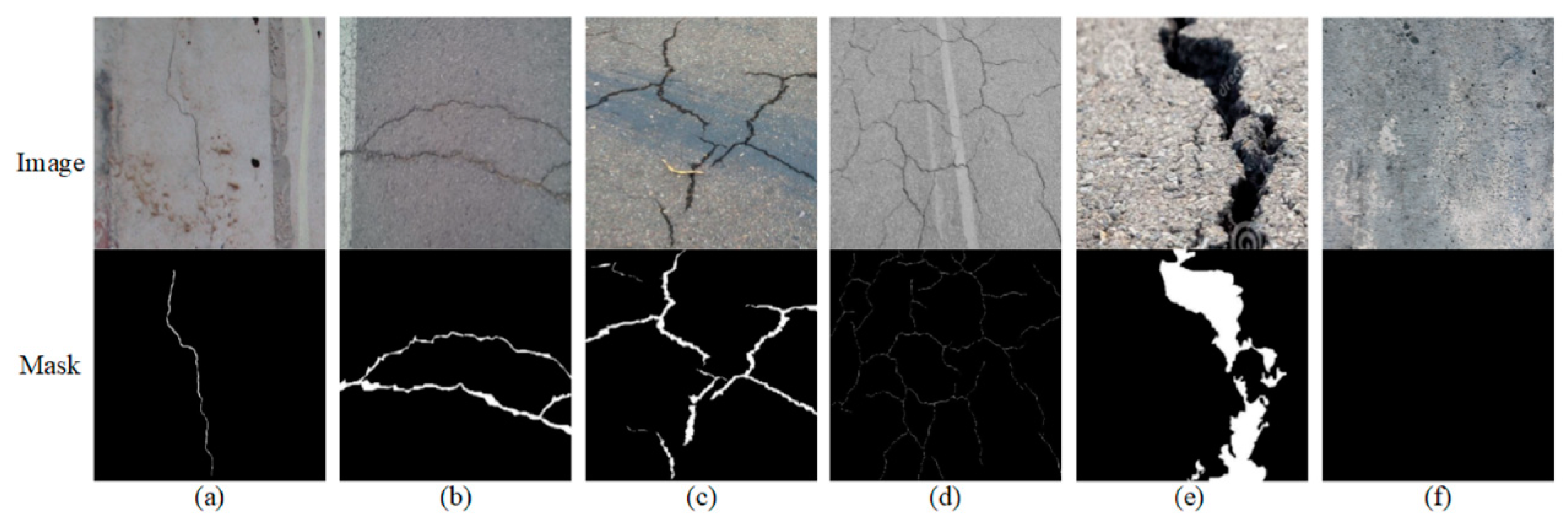
• A public dataset with manual annotations was established, including 7169 crack images with a resolution of 448 × 448. This dataset includes labeled crack images of different scenes and different shapes, as well as non-crack images which are similar to crack images, which can enhance the generalization ability of the model.

2. Methods

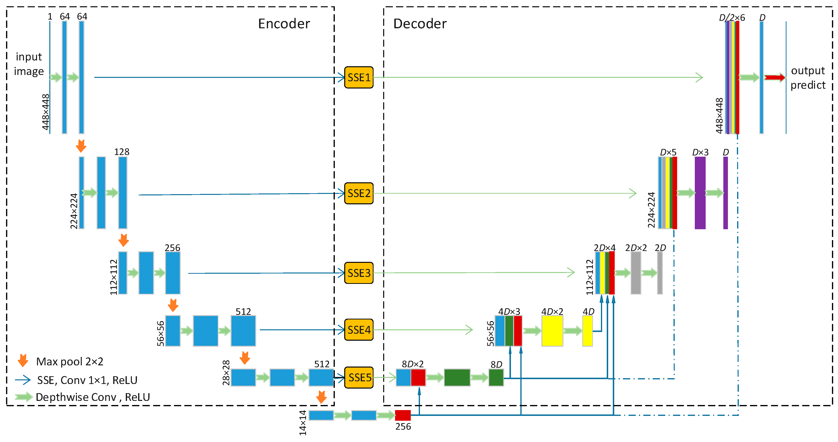
2.1. Model Architecture

The structure of the pixel-level SCCDNet is shown in Figure 1. The model uses the classic Encoder-Decoder [28] structure, in which the Encoder learns the features of images at different scales, and the Decoder obtains predicted images with the same resolution as the input image by combining the feature map in the Encoder module.

As shown in Figure 1, the left dotted box contains the structure of the Encoder. We used 13 convolutional layers pretrained in the VGG-16 network as the main structure of the Encoder. In order to reduce the amount of model parameters without affecting the performance of the model, we used depthwise separable convolution [33] instead of traditional convolution. Each depthwise separable convolution is composed of a Depth-wise (DW) convolution and a Point-wise (PW) convolution, which can reduce the amount of calculation to the original $1/N+1/D_K^2$ without reducing the performance of the model, where N is the number of channels of the output feature map, and $D_K$ is the size of the convolution kernel. In this model, the size of the convolution kernel of all DW convolutions is $3\times 3$, and that of all PW convolutions is $1\times 1$. In order to ensure that the dimension of the output feature map remains unchanged, we set padding = 1 in DW convolutions. In addition, in order to enhance the generalization ability of the crack segmentation model, considering the need to segment cracks of different sizes, we used 5 downsampling operations with a size of $2\times 2$ to reduce the resolution of the feature maps and learn the characteristics of cracks on different scales.

The right dotted box contains the structure of the Decoder. DenseNet [34] proved that establishing short connections between the layers of the network will strengthen feature propagation, encourage feature reuse, alleviate gradient disappearance, and make training more efficient. Inspired by this, we designed a densely connected structure in the Decoder module, reducing the number of channels of each feature map, and improving the performance of the model. The dash-dotted lines indicate the omitted operations. The detailed structure of the Decoder module is detailed in Section 2.3.

Compared to U-Net [27], which directly uses the feature map of the Encoder as the input of the Decoder, Oktay et al. [35] verified that introducing the Attention Gate (AG) model into the connection between the Encoder and the Decoder, allowing the model to automatically focus on targets of different shapes and sizes, while emphasizing the area of interest while suppressing irrelevant area. Therefore, we used the SSE module to connect the Encoder module and the Decoder module. The SSE module plays the role of AG model, and the structure of it is detailed in Section 2.2. In order to further reduce the amounts of parameters, we compressed the number of channels before using the feature map output by the Encoder module as the input of the SSE module. In addition, all activation functions used in the model are the rectified linear unit (ReLU) [36]. The codes of our model are available at https://github.com/543630836/SCCDNet_crack, accessed on 29 May 2021.

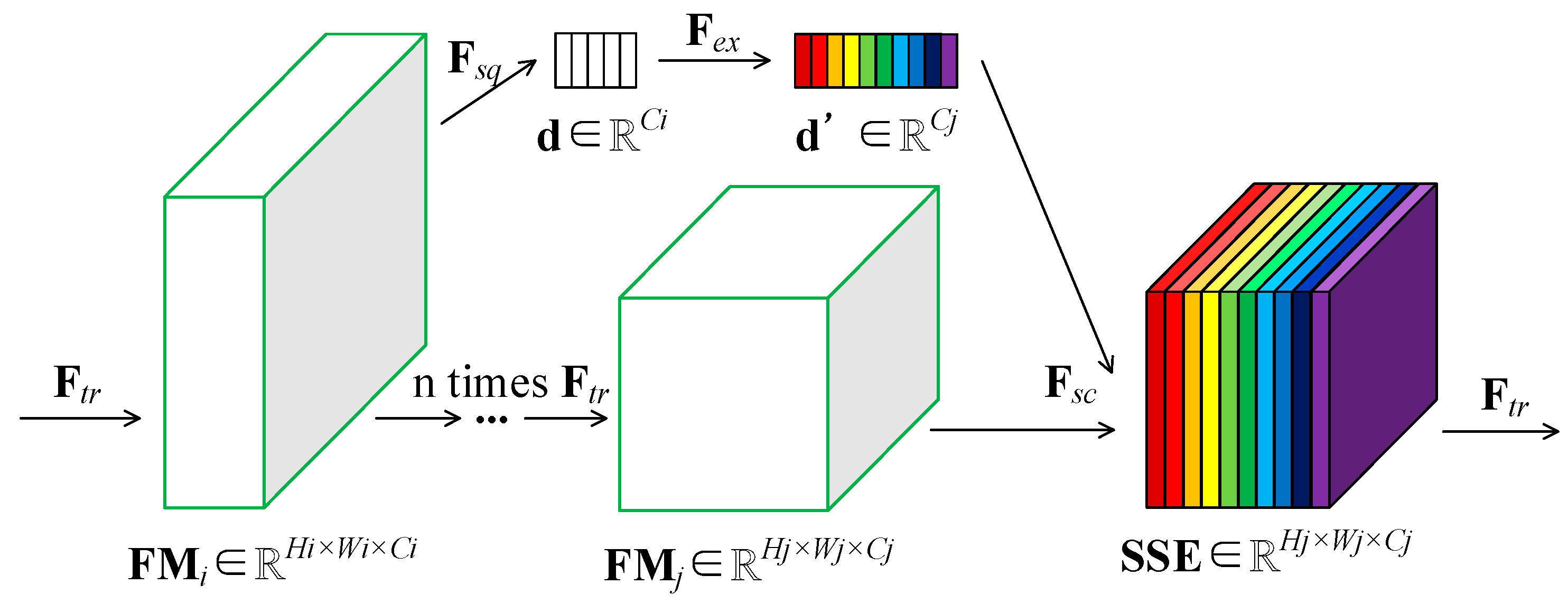
2.2. SSE Module

We designed an embedded SSE module [37] based on the skip-connection and Attention strategy, which is an important part of the SCCDNet. Oktay et al. [35] proved that the AG model is more efficient than the concatenating operation used in U-Net. Inspired by their work, we designed the SSE module to connect the feature map with the same resolution in the Encoder and Decoder. Instead of considering the global feature obtained by the output of early layers directly, the SSE module could emphasize useful channels and suppress useless channels of the feature map, which could alleviate the problem that the correlation of feature maps decreases due to the increase of network depth. This kind of skip-connection strategy is useful for increasing model performance in Encoder-Decoder structures. The SSE module is used to recalibrate the feature map output by the Encoder module, then used as the input of the Decoder module.

The structure of the SSE module is shown in Figure 2. The input of Squeeze operation is the feature map $F{M}_i$, and its spatial dimensions will be aggregated in each channel, that is, use global average pooling, compress the size of size $H_i\times W_i$ in each channel to $1\times 1$, and get the channel-wise feature descriptor $d\in {ℝ}^{C_i}$, the formula is as follows:

$$d_c=F_{sq}\left(F{M}_{ci}\right)=\frac{1}{H_i\times W_i}{{\displaystyle \sum }}_{m=1}^{H_i}{{\displaystyle \sum }}_{n=1}^{W_i}F{M}_{ic}\left(m,n\right),$$

(1)

where $d_c$ is the value of c-th channel in the channel descriptor $d$ and $F{M}_{ic}$ refers to the c-th channel of the feature map $F{M}_i$.

In order to alleviate the gradient irrelevance, we select the deeper feature map $F{M}_j$ to interact with the channel information descriptor $d$ obtained from the output of early layers. However, the number of channels of them are usually different. In order to multiply the two, we have to process $d$ further. The Squeeze is the attention to the spatial dimension and it can obtain the global eigenvalues of each channel; however, it does not consider the relationship between the channels, so the Excitation part uses the gating strategy [38] to focus on establishing the correlation between the channels:

$$d^{\prime }=F_{ex}\left(d,W_1,W_2\right)=\delta \left(W_2\delta \left(W_{1}d\right)\right),$$

(2)

where $d^{\prime }=\left[d_1^{\prime },d_2^{\prime },\dots ,d_c^{\prime },\dots ,d_j^{\prime }\right]$, $\delta$ refers to the ReLU activation function, $W_1\in {ℝ}^{\frac{C_i}{r}\times C_i}$, $W_2\in {ℝ}^{C_j\times \frac{C_i}{r}}$, r is reduction ratio. To build up the correlation between channels, we take the channel descriptor $d$ as the input of two fully-connected layers. The first fully-connected layer changes the number of channels from $C_i$ to $C_i/r$, and the second changes the number of channels from $C_i/r$ to $C_j$, which is the same as the channels number of the feature map $F{M}_j$. The final output of the SSE module is obtained by the following formula:

$$SS{E}_c=F_{sc}\left(F{M}_{jc},d_c^{\prime }\right)=d_c^{\prime }F{M}_{jc},$$

(3)

where $SSE=\left[SS{E}_1,SS{E}_2,\dots ,SS{E}_c,\dots ,SS{E}_j\right]$, $F_{sc}\left(F{M}_{jc},d_c^{\prime }\right)$ refers to channel-wise multiplication between the channel weights $d_c^{\prime }$ and the feature map $F{M}_{jc}$.

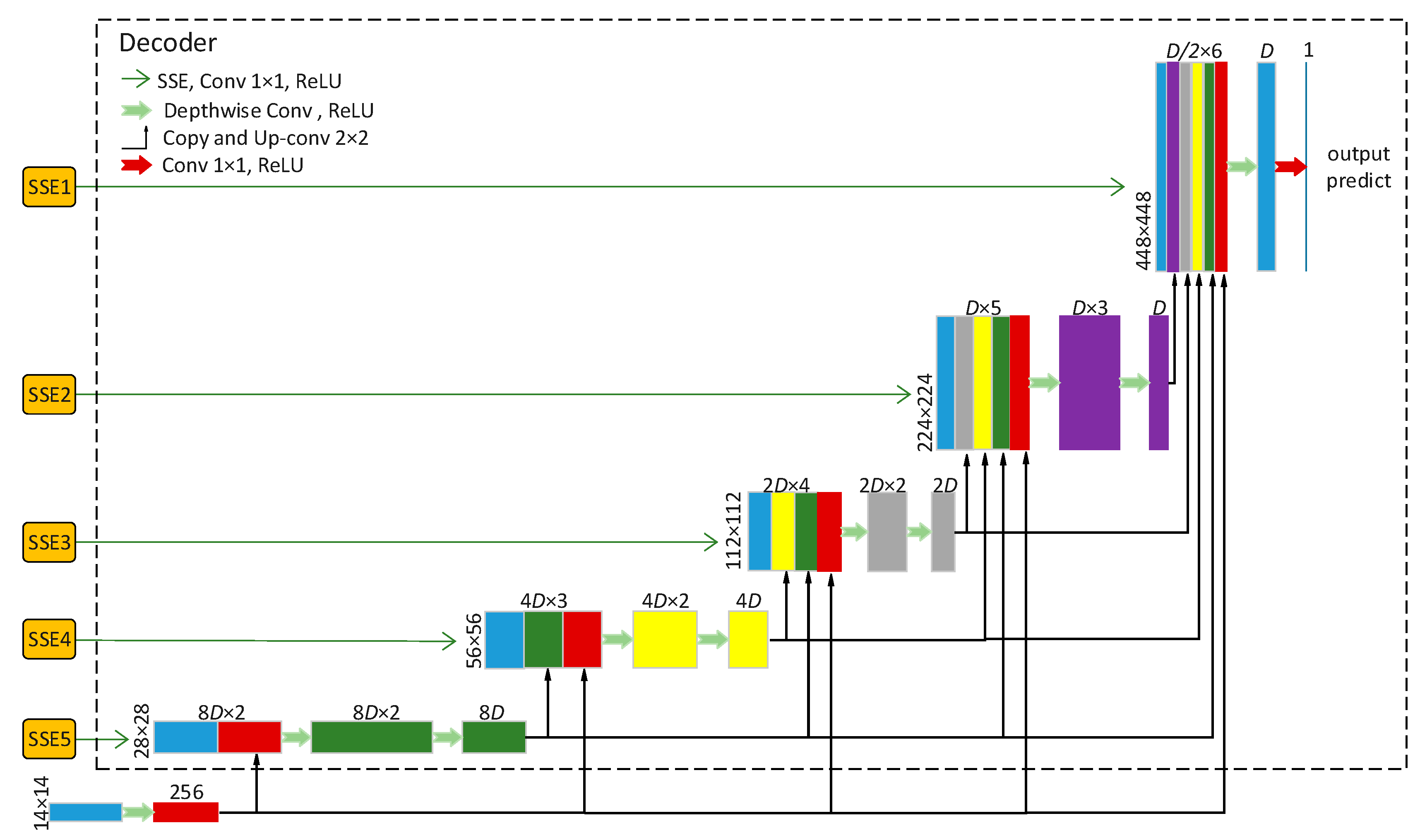
2.3. Decoder Module

The function of the Decoder module is to resize the low-resolution feature map obtained by the Encoder to the same resolution as the input image to achieve pixel-level segmentation of the image. As shown in Figure 3, the dotted box contains the structure diagram of the Decoder. As can be seen from the figure, the Decoder and Encoder can be divided into five parts according to the spatial resolution of the feature map, and each part is composed of two depth wise separable convolutions, which can minimize the complexity of the model compared to conventional convolutions.

In addition to the $14\times 14\times 256$ feature map obtained at the bottom of the module, the input of the Decoder module also includes the result of the feature maps of different spatial resolutions in the Encoder module after being recalibrated by the SSE module. For example, the input of the first part of the Decoder consists of two parts, the first part of the feature map represented by the blue rectangle comes from the output of the SSE5 module, and the size is 28 × 28 × 8D; The other part of the feature map represented by the red rectangle comes from the feature map of the lowest resolution after 2 × 2 deconvolution, whose size is 28 × 28 × 8D. After concatenating two feature maps of the same size, two depth separable convolutions are performed to obtain the output feature map of the first part of the Decoder module.

In order to further alleviate the problem of gradient disappearance as the network depth increases, we establish short connections in the Decoder module. For instance, in addition to the output of the SSE1 module, we use the remaining five output feature maps of the Decoder module as the input of the fifth part of the module. This strategy not only considers all the output feature maps of the Decoder, but also considers that of the Encoder through the SSE module, and will not weaken the features obtained by the shallow network as the depth of the model increases.

2.4. Model Customization

As shown in Figure 1, SCCDNet can be customized by setting different depth values (D), which means the number of channels. The number of model parameters and segmentation accuracy will change with the selection of D. We can customize the model with appropriate D according to the different data set sizes. In this paper, we use SCCD-D# to represent different customized models, where D# represents the value of D. We discuss in detail the influence of parameter D on the number of model’s parameters and segmentation results in Section 3.3, and finally select SCCD-D32 as the best model after experimental verification.

2.5. Loss Function and Hyperparameters

Since the crack detection task can be equivalent to the semantic segmentation problem of two classes, that is, the output of the network is a single-channel probability map of crack prediction. Therefore, we chose the cross-entropy function with sigmoid as the loss function of the model. The formula is as follows:

$$l_n=-w_n\left[y_n·log\sigma \left(x_n\right)+\left(1-y_n\right)\log \left(1-\sigma \left(x_n\right)\right)\right],$$

(4)

where $x_n$ represents the predicted image output by the model, $y_n$ represents the ground truth of the input image, $n$ represents the n-th image in the batch size; $\sigma (·)$ represents the sigmoid function, which can assign the predicted image to a value between 0–1; $w_n$ represents the weight of each loss. When a pixel in the ground truth image belongs to a crack, then $y_n=1$. If the value of the pixel in the predicted image is closer to 1, then the value of $l_n$ is closer to 0, and the training loss is smaller; on the contrary, the value of the pixel is closer to 0, the greater the training loss. Therefore, sigmoid cross entropy is suitable as the loss function of the crack detection task.

The model parameters we tuned are: the size of input images ($448\times 448\times 3$), the size of ground truth ($448\times 448\times 1$). In this paper, we choose SGD optimizer to optimize the entire model and the mini-batch size is 4. The momentum variable is set as 0.9 and it is helpful for stabilizing network training. The weight decay is 0.0001 while the initial learning rate is set as 0.005. We use CosineAnnealingLR [39] strategy to adjust the learning rate during the training and set T_max as 5, which means that the change period of learning rate is 10. This strategy is helpful for training loss to escape from local minimum point. In order to ensure that the model is fully trained, we have to choose appropriate stopping criteria for the training process. The specific strategy is: if the loss of validation set dose not decrease in 10 epochs, the model is considered to be fully trained. Further, the maximum epoch is set as 100.

3. Results and Experimental Evaluations

SCCDNet is built with python3.6 under the framework of pytorch1.4.0. All training and testing are performed under the following hardware environment:

(a)

CPU: Intel(R) Core(TM) i9-7980XE;

(b)

GPU: NVIDIA 2080Ti GPU;

(c)

RAM: 32 GB.

3.1. Dataset

Currently, there is no consistent public dataset for pixel-level crack segmentation task, so it is difficult to compare other networks on the same dataset. Most of the previous papers train and test their networks on small datasets established by themselves, which cannot verify the generalization ability of the model. Therefore, we set up a large-scale public dataset to verify the effectiveness of the network. This dataset consists of 7169 images with manually annotated labels with a resolution of $448\times 448$. Some typical crack images and their labels are shown in Figure 4. It can be seen that the data set contains crack images of different environments, different shooting distances, and different forms, covering the common crack characteristics to the greatest extent. The images in the dataset come from published datasets [9,30,40,41,42], crack images on the Internet, and images of similar crack objects.

The dataset is divided into two parts: training set and test set: the training set contains 6164 input images and label images, including 4965 crack images and 1199 no crack images; the test set contains 1005 crack images and label images, including 793 crack images and 212 no crack images. In addition to the various crack images, we add about 20% of the no crack images to the dataset. The purpose is to strengthen the anti-interference ability of the model and reduce the probability of detecting environmental objects as cracks.

3.2. Evaluation Matrix

In order to quantitatively evaluate the accuracy of crack segmentation, we need to select appropriate evaluation indicators. First, in crack detection sphere, we use the following evaluation indicators:

$$Precision=\frac{TruePositives}{TruePositives+FalsePositives},$$

(5)

$$Recall=\frac{TruePositives}{TruePositives+FalseNegatives},$$

(6)

$$F-score=\frac{2\times Precision\times Recall}{Precision+Recall}.$$

(7)

Precision represents the proportion of pixels that are correctly detected as cracks, which reflects the impact of false detection on the results; Recall represents the proportion of real crack pixels that are correctly detected, which reflects the impact of missed detection on the results; F-score represents the harmonic average of the two, which reflects the comprehensive ability of the model to resist false detection and missed detection.

In addition, we also introduce two common evaluation criteria in the sphere of semantic segmentation, Dice and Intersection over union (IoU) [16]. Let $X\left(i,j\right)$ be the segmented image output by the model, and $Y\left(i,j\right)$ be the corresponding truth image in the data set, where $i\in \left[0,H\right]$, $j\in \left[0,W\right]$, $H$ and $W$ are the length and width of the image respectively, the formula is:

$$Dice=\frac{2\left|{{\displaystyle \sum }}_i{{\displaystyle \sum }}_{j}X\left(i,j\right)·Y\left(i,j\right)\right|}{\left|{{\displaystyle \sum }}_i{{\displaystyle \sum }}_{j}X\left(i,j\right)\right|+\left|{{\displaystyle \sum }}_i{{\displaystyle \sum }}_{j}Y\left(i,j\right)\right|},$$

(8)

$$IoU=\frac{\left|{{\displaystyle \sum }}_i{{\displaystyle \sum }}_{j}X\left(i,j\right)·Y\left(i,j\right)\right|}{\left|{{\displaystyle \sum }}_i{{\displaystyle \sum }}_j\left[\left(X\left(i,j\right)+Y\left(i,j\right)\right)-X\left(i,j\right)·Y\left(i,j\right)\right]\right|}.$$

(9)

In addition to measuring the segmentation accuracy of the model, the complexity of the model is also an important indicator. We select model parameters and Floating Point of Operations (FLOPs) to represent the complexity of the model. The formulas are as follows:

$$Parameters=\left(D_K\times D_K\times M\right)\times N+N,$$

(10)

$$FLOPs=\left[\left(D_K\times D_K\times M\right)\times N+N\right]\times \left(H\times W\right),$$

(11)

where $D_K$ represents the size of the convolution kernel, $M$ and $N$ represent the number of channels of the input feature map and output feature map, respectively, and $H$ and $W$ represent the length and width of the output feature map, respectively.

3.3. Segmentation Result

As mentioned in Section 2.4, SCCDNet can customize models with different parameters by selecting different depth values. We select the models constructed with D = 4, D = 8, D = 16, D = 32, and D = 64, respectively, for training, and compare their performances in segmentation accuracy and model complexity. In addition, in order to further verify the advantages of SCCDNet, we choose the advanced approach DeepCrack [31], U-Net [27], and SegNet [28] to compare with the model we designed. U-Net and SegNet use the Encoder-Decoder structure, and the comparison results are shown in

Table 1. Segmentation results of different models. The best scores are in bold.

Models	Precision	Recall	F-Score	Dice	IoU	FLOPs/G	Parameters/M
U-Net	0.6953	0.8056	0.7464	0.7185	0.6002	111.632	44.021
SegNet	0.6483	0.7402	0.6912	0.6184	0.5015	30.703	29.444
DeepCrack	0.6761	0.4489	0.5396	0.3951	0.3166	61.280	58.858
SCCD-D4	0.7336	0.7320	0.7328	0.6959	0.5773	61.590	30.161
SCCD-D8	0.7114	0.8467	0.7732	0.7511	0.6362	61.817	30.302
SCCD-D16	0.7234	0.8223	0.7697	0.7485	0.6324	62.533	30.663
SCCD-D32	0.7294	0.8296	0.7763	0.7541	0.6402	65.004	31.705
SCCD-D64	0.7302	0.8278	0.7760	0.7495	0.6372	74.108	35.066

.

It can be seen from Table 1 that with the increase of D, the Parameters and FLOPs are increasing. However, except for SCCD-D64, the complexity of the other models is not much different. Among all the models of SCCDNet, the precision of the model is the highest when D = 4. The proportion of false positives of the model is the lowest at this time, so the ability to resist false detection is the strongest. When D = 8, the Recall of the model is the highest. At this time, the false negative of the model is the lowest, and the ability to resist missed detection is the strongest. When D = 32, the highest F-score, Dice, and IoU are obtained. Since F-score is the harmonic average of Precision and Recall, the model has the strongest ability to resist false detection and missed detection at the same time. Although SCCD-D64 has the largest amounts of parameters, its segmentation results are slightly worse than SCCD-D32, except Precision.

The experimental results are consistent with the theoretical analysis. The change of D determines the number of channels and parameters of the Decoder module. Theoretically, the performance of the model will improve with the increase of the model parameters, but when the model’s ability has a large redundancy relative to the scale of the dataset, there will be an over-fitting problem, and the performance of a model with more parameters will not improve or even decrease compared to the model with less parameter. The results also show that as D increases from 4 to 32, the amounts of parameters and segmentation accuracy of the model is steadily improving; however, when D increases to 64, the amounts of parameters greatly increase. At the same time, the accuracy of the model is slightly lower than that when D = 32, and the model is over-fitting at this time. Since continuing to increase D will introduce more parameters, we choose SCCD-32 as the best model.

Compared with U-Net, SCCD-D32 improves Precision, Recall, F-score, Dice, and IoU by 4.9%, 3.0%, 4.0%, 5.0%, and 6.7%, respectively, and reduces FLOPs and Parameters by 41.8% and 28.0%, respectively, which improves the accuracy of crack segmentation under the premise of greatly reducing the complexity of the model; compared with SegNet, although the complexity of the model is increased, the accuracy of crack segmentation is greatly improved. The precision, Recall, F-score, Dice, and IoU are increased by 9.5%, 20.5%, 14.6%, 27.4%, and 34.1%, respectively. Compared with other models, DeepCrack shows relatively poor performance, because it is designed for the task of small crack dataset. The structure of DeepCrack is hard to deal with such a large dataset having crack images obtained from different environment. Therefore, SCCDNet greatly improves the accuracy of crack segmentation on the complex dataset while reducing the complexity of the model as much as possible.

The visualization of experimental results of typical models is shown in Figure 5. It can be seen that SCCD-D32 can completely detect the cracks in the input image. Compared to the output of SCCD-D32, fine cracks detected by other models will break in the middle, or even cannot be detected, which means that the models’ anti-miss detection ability needs to be improved. In addition, SegNet and DeepCrack will falsely detect other stains as cracks, which means that the anti-error detection ability needs to be improved. Although SCCD-D32 shows the strongest capability in all models, we notice that it cannot detect some detail texture on the edge of the crack. This may be due to the excessive number of pooling layers, resulting in the loss of texture details. We will consider designing a more efficient structure to utilize the detail texture of the feature map in the Encoder module.

3.4. 5-Fold Cross-Validation

Although the dataset we constructed is larger than that used by other researchers, it is still smaller than the common semantic segmentation dataset. Therefore, in order to prevent the over-fitting problem, we use a 5-fold cross-validation method.

We divide the training set into five parts and select one part as the validation set, in turn, while the remaining four as the training set so that a total of five training sessions are performed. In theory, each image in the dataset will be selected as the validation set. Compared with only a small part of the images can be used as the verification set, the 5-fold cross-validation can ensure that each image in the training set will be used as the verification set, which can further verify the generalization ability of the model and prevent the randomness of the selected validation set from affecting the results.

In order to verify the ability of the SCCD-D32 model, we choose the SCCD-16, SCCD-64, U-Net, and SegNet models for 5-fold cross-validation. The average results are shown in

Table 2. Results of 5-fold cross-validation. The best average scores are in bold.

Models	m-Train_Loss	m-Valid_Loss	m-Precision	m-Recall	m-F-Score	m-Dice	m-IoU
U-Net	0.0245	0.0284	0.6901	0.8069	0.7439	0.7160	0.5967
SegNet	0.0275	0.0404	0.6349	0.7592	0.6908	0.6226	0.5061
SCCD-D16	0.0248	0.0363	0.7161	0.8246	0.7103	0.6462	0.5320
SCCD-D32	0.0209	0.0270	0.7199	0.8300	0.7710	0.7457	0.6316
SCCD-D64	0.0203	0.0270	0.7192	0.8320	0.7714	0.7441	0.6308

. M-train_loss represents the average training losses obtained from five training sessions; m-valid_loss represents the average verification losses obtained from five training sessions; the rest of the evaluation criteria are the average values of test results obtained after five training sessions. It can be seen from the table that SCCD-D64 has the lowest average training loss, and SCCD-D32 and SCCD-D64 have both the lowest average verification loss. In the test evaluation indicators, SCCD-D32 gets the highest m-Precision, m-Dice and m-IoU, and SCCD-D64 get the highest m-Recall and m-F-score. The results of the 5-fold cross-validation are basically consistent with the results obtained in Table 1. SCCD-D32 and SCCD-D64 both show better crack segmentation performance than other models, while SCCD-D32 saves a lot of Parameters and FLOPs compared to SCCD-D64. Therefore, we choose SCCD-D32 as the best model.

3.5. Ablation Study and Discussion

In this part, we discuss the crack segmentation results obtained after the SCCDNet model is constructed in different ways. We focus on the impact of the SSE module, the Decoder module, and the depthwise separable convolution on the overall model.

3.5.1. Ablation Analysis of the SSE Module

In Section 2.2, we specifically introduced the structure and function of the SSE module. In order to prove its contribution to the model, we compare the effects of different connection strategies on the accuracy of crack segmentation. In order to prove the generalization of the model, we also use 5-fold cross-validation to prove the influence of the SSE module on the performances. The results are shown in

Table 3. Results of different SSE modules. The best average scores are in bold.

Models	m-Precision	m-Recall	m-F-Score	m-Dice	m-IoU	FLOPs/G	Parameters/M
None-SSE	0.7153	0.8024	0.7563	0.7364	0.6181	64.997	30.875
SSE1	0.7192	0.8084	0.7612	0.7409	0.6230	64.997	31.269
SSE2	0.7139	0.8046	0.7566	0.7379	0.6187	64.997	31.203
SSE3	0.7126	0.8168	0.7612	0.7387	0.6211	64.998	30.957
SSE4	0.7326	0.8017	0.7656	0.7489	0.6316	64.998	30.895
SSE5	0.7313	0.8046	0.7662	0.7465	0.6297	65.000	30.880
Fully-SSE	0.7294	0.8296	0.7763	0.7541	0.6402	65.004	31.705

.

As shown in Table 3, None-SSE represents the model in Figure 1 without any SSE module, that is, completely eliminates the contribution of the SSE module; SSE1 represents the model that only remains the SSE1 module which connects two feature maps with a resolution of 448×448, while SSE2, SSE3, SSE4, SSE5, respectively, indicate that only the corresponding SSE modules in Figure 1 remained, and the influence of other SSE modules on the results is excluded. Fully-SSE means that all 5 SSE modules remained, and the network structure is shown in Figure 1. In order to prove the generalization of the model, we also use 5-fold cross-validation to prove the influence of the SSE module on the experimental results.

As shown in Table 3, compared to None-SSE, SSE1, SSE2, and SSE3 do not greatly improve the model performance. The reason is that the feature maps connected by the three modules are too far apart, so the difference between the features is too large. Although the value of the shallow feature map is recalibrated through the attention gate, it is difficult to find similar features in the subsequent learning after concatenating, so the improvement of model performance is limited; SSE4 and SSE5 improve m-Precision more greatly and improve m-Recall less. Therefore, when using the SSE module to connect two feature maps that are close, the model’s ability to resist error detection is enhanced significantly. In addition, compared with the None-SSE model, all models with the SSE module have improved m-F-score, m-Dice, and m-IoU, which enhances the model’s crack segmentation capabilities. The Fully-SSE model enhances the model’s ability to resist error detection and missed detection and has obtained the greatest evaluation performances except for m-Precision. We verified that all SSE modules can improve the performance of the model. Although some improvements are not obvious, considering that the SSE module basically does not increase the amount of model parameters, we use Fully-SSE as the best model.

3.5.2. Ablation Analysis of the Decoder Module

In Section 2.3, we specifically introduce the structure and characteristics of the Decoder module. In order to verify the effectiveness of our Decoder module, we design a comparative experiment as shown in

Table 4. Results of different decoder modules. The best average scores are in bold.

Models	m-Precision	m-Recall	m-F-Score	m-Dice	m-IoU	FLOPs/G	Parameters/M
Normal Decoder	0.6929	0.8150	0.7489	0.7232	0.6040	111.639	45.245
Dense Decoder	0.7294	0.8296	0.7763	0.7541	0.6402	65.004	31.705

. Between them, the Normal Decoder uses the most common Decoder module of U-Net [27], and the Dense Decoder uses the densely connected Decoder module as shown in Figure 3. Furthermore, we unsure the other parts of the models are the same. In order to prove the generalization of the model, we also use 5-fold cross-validation to compare the influence of the Decoder module on the results.

It can be seen from the table that the Dense Decoder module we designed greatly improves the accuracy of crack segmentation compared to the Normal Decoder module, and greatly reduces the complexity of the model. Specifically, m-Precision, m-Recall, mF-score, m-Dice, and m-IoU increase by 5.3%, 1.8%, 3.7%, 4.3%, and 6.0%, respectively; FLOPs and Parameters decrease by 41.8% and 29.9%, respectively. The dense connection of the Decoder module enhances the gradient correlation of the model and improves the performance of the model by utilizing feature maps from early layers. This allows us to reduce the number of convolutions of each layer and reduce the amount of model parameters.

3.5.3. Ablation Analysis of the Depthwise Separable Convolution

In order to further reduce the complexity of the model, we use depthwise separable convolution in the model, as shown in Figure 1. In order to verify the contribution of the depthwise separable convolution in the network and to prove the generalization of the model, we designed the 5-fold cross-validation shown in

Table 5. Results of different convolution strategies. The best average scores are in bold.

Models	m-Precision	m-Recall	m-F-Score	m-Dice	m-IoU	FLOPs/G	Parameters/M
Normal Conv	0.7281	0.8112	0.7674	0.7485	0.6310	83.786	39.499
D-S Conv	0.7294	0.8296	0.7763	0.7541	0.6402	65.004	31.705

. Between them, Normal Conv represents the SCCDNet that uses conventional convolutions; D-S Conv represents the SCCDNet that uses depthwise separable convolutions.

Compared with using conventional convolution, it can be seen from the table that using depthwise separable convolution greatly reduces the complexity of the model and further improves the accuracy of crack segmentation. This also proves that the spatial dimension and channel dimension in the convolution kernel are decoupled, that is, the conventional convolution convolutes the spatial dimension and channel dimension at the same time, and separates them into the operation of spatial dimension and channel dimension in turn, which can reduce the complexity of the model and improve the performance of the model. Specifically, FLOPs and Parameters decrease by 22.4% and 19.7%, respectively, while m-Precision, m-Recall, m-F-score, m-Dice, and m-IoU increase by 0.2%, 2.3%, 1.2%, 0.7%, and 1.5%, respectively.

4. Conclusions

In this paper, we design an end-to-end crack segmentation network based on CNNs, which can detect the crack image in pixel-level. SCCDNet is composed of the Encoder module using 13 convolution layers pretrained in VGG-16 network, the Decoder module with dense connection structure, and the SSE module connecting the Encoder and the Decoder. In order to further reduce the complexity of the model, we replace all convolutions with depthwise separable convolutions. In practical applications, the aim of crack detection is to detect different forms of cracks in various environments. However, most of the existing crack detection models detect a single form of cracks in a dataset collected in a single environment, and the dataset is small. Therefore, we established a dataset with 7169 labeled images (crack images with different textures collected in different environments) and conducted training and testing on this dataset. We will publish the code and dataset of the model used in this paper, so as to support other researchers to compare with our model. We prove the performance of our model by comparing SCCDNet with other popular models. Results show that SCCD-D32 is the best model in the SCCDNet series, and its performance in crack segmentation accuracy and model parameters is better than other models. Although the overall performance of the SCCD-D32 model is excellent, its m-Precision can only reach 0.7294, which is much lower than the 0.8296 of m-Recall, which proves that the ability to resist error detection is weaker than the ability to resist missed detection. Therefore, we will continue to conduct in-depth research on improving the model’s ability to resist error detection.

References

- Alipour, M.; Harris, D.K. Increasing the robustness of material-specific deep learning models for crack detection across different materials. Eng. Struct. 2020, 206, 110157. [Google Scholar] [CrossRef]
- Oliveira, H.; Correia, P.L. Automatic road crack segmentation using entropy and image dynamic thresholding. In Proceedings of the 17th European Signal Processing Conference (EUSIPCO 2009), Glasgow, Scotland, 24–28 August 2009; IEEE: New York, NY, USA, 2009; pp. 622–626. [Google Scholar]
- Elbehiery, H.; Hefnawy, A.; Elewa, M. Surface defects detection for ceramic tiles using image processing and morphological techniques. IJREAS 2005, 2, 1307–1322. [Google Scholar]
- Georgieva, K.; Koch, C.; König, M. Wavelet transform on multi-GPU for real-time pavement distress detection. In Computing in Civil Engineering; American Society of Civil Engineers (ASCE): Reston, VA, USA, 2015; pp. 99–106. [Google Scholar]
- Zhang, A.; Li, Q.; Wang, K.C.; Qiu, S. Matched filtering algorithm for pavement cracking detection. Transp. Res. Rec. J. Transp. Res. Board 2013, 2367, 30–42. [Google Scholar] [CrossRef]
- Li, Q.; Liu, X. In Novel approach to pavement image segmentation based on neighboring difference histogram method. In Proceedings of the 2008 Congress on Image and Signal Processing, Sanya, China, 27–30 May 2008; IEEE: Washington, DC, USA, 2008; pp. 792–796. [Google Scholar]
- Chun, P.J.; Izumi, S.; Yamane, T. Automatic detection method of cracks from concrete surface imagery using two-step light gradient boosting machine. Comput. Aided Civ. Infrastruct. Eng. 2021, 36, 61–72. [Google Scholar] [CrossRef]
- Li, Q.; Zou, Q.; Zhang, D.; Mao, Q. FoSA: F* seed-growing approach for crack-line detection from pavement images. Image Vis. Comput. 2011, 29, 861–872. [Google Scholar] [CrossRef]
- Zou, Q.; Cao, Y.; Li, Q.; Mao, Q.; Wang, S. CrackTree: Automatic crack detection from pavement images. Pattern Recognit. Lett. 2012, 33, 227–238. [Google Scholar] [CrossRef]
- LeCun, Y.; Bottou, L.; Bengio, Y.; Haffner, P. Gradient-based learning applied to document recognition. Proc. IEEE 1998, 86, 2278–2324. [Google Scholar] [CrossRef]
- Zhang, A.; Wang, K.C.; Li, B.; Yang, E.; Dai, X.; Peng, Y.; Fei, Y.; Liu, Y.; Li, J.Q.; Chen, C. Automated pixel-level pavement crack detection on 3D asphalt surfaces using a deep-learning network. Comput. Civ. Infrastruct. Eng. 2017, 32, 805–819. [Google Scholar] [CrossRef]
- Sermanet, P.; Chintala, S.; LeCun, Y. Convolutional neural networks applied to house numbers digit classification. In Proceedings of the 21st International Conference on Pattern Recognition (ICPR2012), Tsukuba, Japan, 11–15 November 2012; IEEE: Washington, DC, USA, 2012; pp. 3288–3291. [Google Scholar]
- He, K.; Zhang, X.; Ren, S.; Sun, J. Deep residual learning for image recognition. In Proceedings of the IEEE Conference on Computer Vision and Pattern Recognition, Las Vegas, NV, USA, 27–30 June 2016; IEEE: Washington, DC, USA, 2016; pp. 770–778. [Google Scholar]
- Redmon, J.; Farhadi, A. YOLO9000: Better, faster, stronger. In Proceedings of the IEEE Conference on Computer Vision and Pattern Recognition, Honolulu, HI, USA, 21–26 July 2017; pp. 7263–7271. [Google Scholar]
- Wang, L.; Xiong, Y.; Wang, Z.; Qiao, Y.; Lin, D.; Tang, X.; Van Gool, L. Temporal segment networks: Towards good practices for deep action recognition. In Proceedings of the 14th European Conference on Computer Vision, Amsterdam, The Netherlands, 11–14 October 2016; Springer: Berlin/Heidelberg, Germany, 2016; pp. 20–36. [Google Scholar]
- Long, J.; Shelhamer, E.; Darrell, T. Fully convolutional networks for semantic segmentation. In Proceedings of the IEEE Conference on Computer Vision and Pattern Recognition (CVPR), Boston, MA, USA, 7–12 June 2015; IEEE: Washington, DC, USA, 2015; pp. 3431–3440. [Google Scholar]
- Zheng, S.; Jayasumana, S.; Romera-Paredes, B.; Vineet, V.; Su, Z.; Du, D.; Huang, C.; Torr, P.H. Conditional random fields as recurrent neural networks. In Proceedings of the IEEE International Conference on Computer Vision, (CVPR), Boston, MA, USA, 7–12 June 2015; IEEE: Washington, DC, USA, 2015; pp. 1529–1537. [Google Scholar]
- Cha, Y.J.; Choi, W.; Büyüköztürk, O.J. Deep learning-based crack damage detection using convolutional neural networks. Comput. Aided Civ. Infrastruct. Eng. 2017, 32, 361–378. [Google Scholar] [CrossRef]
- Zhang, L.; Yang, F.; Zhang, Y.D.; Zhu, Y.J. Road crack detection using deep convolutional neural network. In Proceedings of the 2016 IEEE International Conference on Image Processing (ICIP), Phoenix, AZ, USA, 25–28 September 2016; IEEE: Washington, DC, USA, 2016; pp. 3708–3712. [Google Scholar]
- Soukup, D.; Huber-Mörk, R. Convolutional neural networks for steel surface defect detection from photometric stereo images. In Proceedings of the International Symposium on Visual Computing, Las Vegas, NV, USA, 8–10 December 2014; Springer: Berlin/Heidelberg, Germany, 2014; pp. 668–677. [Google Scholar]
- Kaseko, M.S.; Ritchie, S.G. A neural network-based methodology for pavement crack detection and classification. Transp. Res. Part C Emerg. Technol. 1993, 1, 275–291. [Google Scholar] [CrossRef]
- Chou, J.; O’Neill, W.A.; Cheng, H. Pavement distress classification using neural networks. In Proceedings of the IEEE International Conference on Systems, Man and Cybernetics, San Antonio, TX, USA, 2–5 October 1994; IEEE: Washington, DC, USA, 1994; pp. 397–401. [Google Scholar]
- Hsu, C.-J.; Chen, C.-F.; Lee, C.; Huang, S.-M. Airport pavement distress image classification using moment invariant neural network. In Proceedings of the 22nd Asian Conference on Remote Sensing and processing (CRISP), Singapore, 5–9 November 2001; pp. 200–250. [Google Scholar]
- Nguyen, T.S.; Avila, M.; Begot, S. Automatic detection and classification of defect on road pavement using anisotropy measure. In Proceedings of the 2009 17th European Signal Processing Conference, Glasgow, UK, 24–28 August 2009; IEEE: Washington, DC, USA, 2009; pp. 617–621. [Google Scholar]
- Moussa, G.; Hussain, K. A new technique for automatic detection and parameters estimation of pavement crack. In Proceedings of the 4th International Multi-Conference on Engineering Technology Innovation (IMETI), Orlando, FL, USA, 19–22 July 2011. [Google Scholar]
- Daniel, A.; Preeja, V. Automatic road distress detection and analysis. Int. J. Comput. Appl. 2014, 101, 18–23. [Google Scholar] [CrossRef]
- Ronneberger, O.; Fischer, P.; Brox, T. U-net: Convolutional networks for biomedical image segmentation. In Proceedings of the International Conference on Medical Image Computing and Computer-Assisted Intervention, Munich, Germany, 5–9 October 2015; Springer: Berlin/Heidelberg, Germany, 2015; pp. 234–241. [Google Scholar]
- Badrinarayanan, V.; Kendall, A.; Cipolla, R. Segnet: A deep convolutional encoder-decoder architecture for image segmentation. IEEE Trans. Pattern Anal. Mach. Intell. 2017, 39, 2481–2495. [Google Scholar] [CrossRef] [PubMed]
- Yamane, T.; Chun, P. Crack detection from a concrete surface image based on semantic segmentation using deep learning. J. Adv. Concr. Technol. 2020, 18, 493–504. [Google Scholar] [CrossRef]
- Fei, Y.; Wang, K.C.; Zhang, A.; Chen, C.; Li, J.Q.; Liu, Y.; Yang, G.; Li, B. Pixel-level cracking detection on 3D asphalt pavement images through deep-learning-based CrackNet-V. IEEE Trans. Intell. Transp. Syst. 2019, 21, 273–284. [Google Scholar] [CrossRef]
- Liu, Y.; Yao, J.; Lu, X.; Xie, R.; Li, L. DeepCrack: A deep hierarchical feature learning architecture for crack segmentation. Neurocomputing 2019, 338, 139–153. [Google Scholar] [CrossRef]
- Choi, W.; Cha, Y.-J. SDDNet: Real-time crack segmentation. IEEE Trans. Ind. Electron. 2019, 67, 8016–8025. [Google Scholar] [CrossRef]
- Howard, A.G.; Zhu, M.; Chen, B.; Kalenichenko, D.; Wang, W.; Weyand, T.; Andreetto, M.; Adam, H. Mobilenets: Efficient Convolutional Neural Networks for Mobile Vision Applications. 2017. Available online: https://arxiv.org/abs/1704.04861 (accessed on 26 April 2021).
- Huang, G.; Liu, Z.; Van der Maaten, L.; Weinberger, K.Q. Densely connected convolutional networks. In Proceedings of the IEEE Conference on Computer Vision and Pattern Recognition, Honolulu, HI, USA, 21–26 July 2017; IEEE: Washington, DC, USA, 2017; pp. 4700–4708. [Google Scholar]
- Oktay, O.; Schlemper, J.; Folgoc, L.L.; Lee, M.; Heinrich, M.; Misawa, K.; Mori, K.; McDonagh, S.; Hammerla, N.Y.; Kainz, B. Attention u-net: Learning where to look for the pancreas. In Proceedings of the 1st Conference on Medical Imaging with Deep Learning (MIDL 2018), Amsterdam, The Netherlands, 4–6 July 2018. [Google Scholar]
- Nair, V.; Hinton, G.E. In Rectified linear units improve restricted boltzmann machines. In Proceedings of the 27th International Conference on Machine Learning, Haifa, Israel, 21–24 June 2010. [Google Scholar]
- Li, H.; Xu, H.; Tian, X.; Wang, Y.; Cai, H.; Cui, K.; Chen, X. Bridge Crack Detection Based on SSENets. Appl. Sci. 2020, 10, 4230. [Google Scholar] [CrossRef]
- Hu, J.; Shen, L.; Sun, G. Squeeze-and-excitation networks. In Proceedings of the IEEE Conference on Computer Vision and Pattern Recognition, Salt Lake City, UT, USA, 18–23 June 2018; IEEE: Washington, DC, USA, 2018; pp. 7132–7141. [Google Scholar]
- Loshchilov, I.; Hutter, F. SGDR: Stochastic gradient descent with warm restarts. 2016. Available online: https://arxiv.org/abs/1608.03983 (accessed on 13 August 2016).
- Fan, R.; Bocus, M.J.; Zhu, Y.; Jiao, J.; Wang, L.; Ma, F.; Cheng, S.; Liu, M. Road crack detection using deep convolutional neural network and adaptive thresholding. In Proceedings of the 2019 IEEE Intelligent Vehicles Symposium (IVS), Paris, France, 9–12 June 2019; IEEE: Washington, DC, USA, 2019; pp. 474–479. [Google Scholar]
- Eisenbach, M.; Stricker, R.; Seichter, D.; Amende, K.; Debes, K.; Sesselmann, M.; Ebersbach, D.; Stoeckert, U.; Gross, H.-M. How to get pavement distress detection ready for deep learning? A systematic approach. In Proceedings of the 2017 International Joint Conference on Neural Networks (IJCNN), Anchorage, AL, USA, 14–19 May 2017; IEEE: Washington, DC, USA, 2017; pp. 2039–2047. [Google Scholar]
- Shi, Y.; Cui, L.; Qi, Z.; Meng, F.; Chen, Z. Automatic road crack detection using random structured forests. IEEE Trans. Intell. Transp. Syst. 2016, 17, 3434–3445. [Google Scholar] [CrossRef]