
Eye State Identification Based on Discrete Wavelet Transforms

 ,
,  , ,
, , 
Abstract
Featured Application
Abstract
1. Introduction
2. Theoretical Background
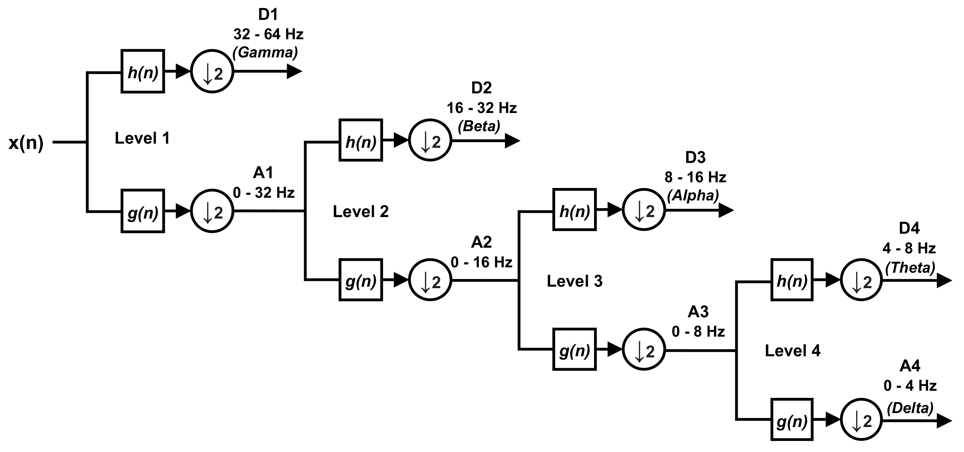
2.1. Wavelet Transform
2.2. Linear Discriminant Analysis
3. Proposed System
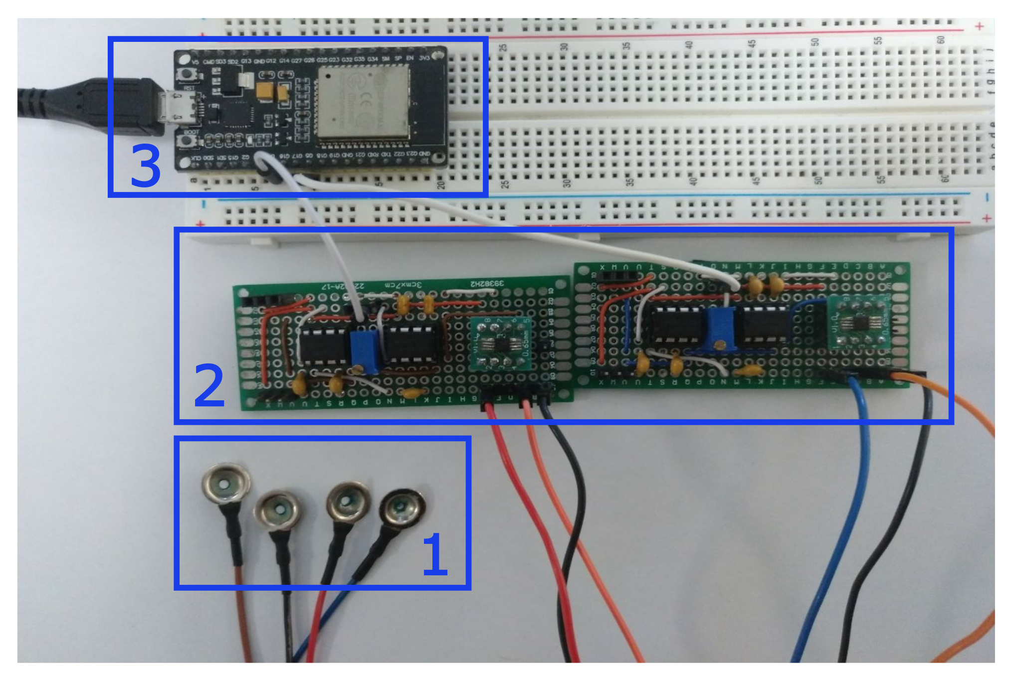
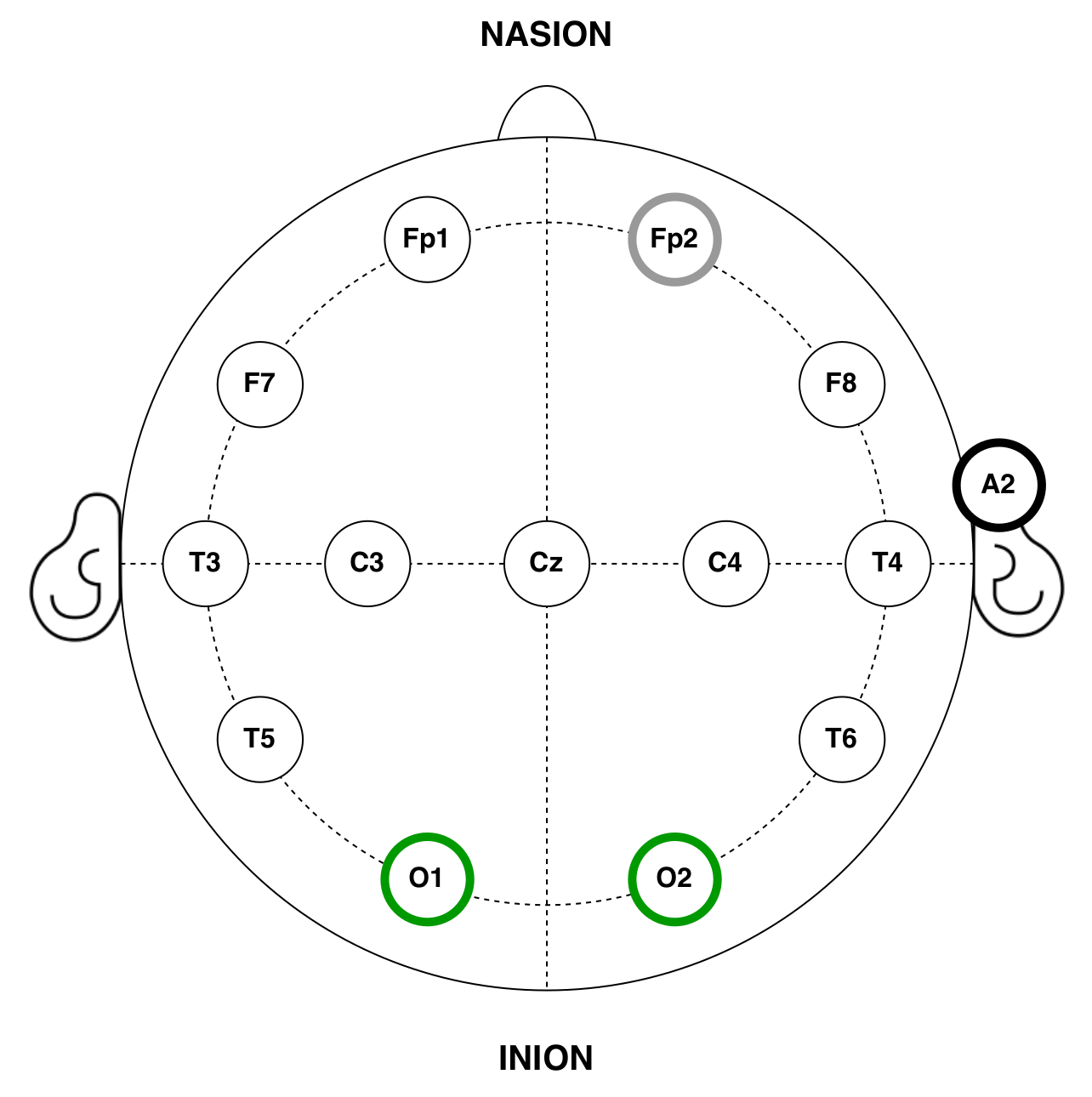
3.1. EEG Device
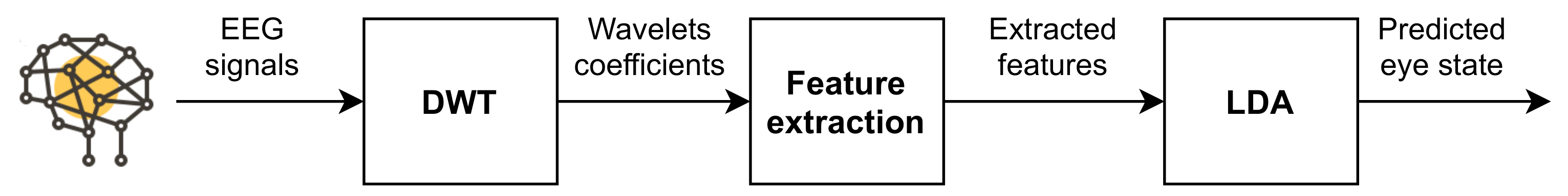
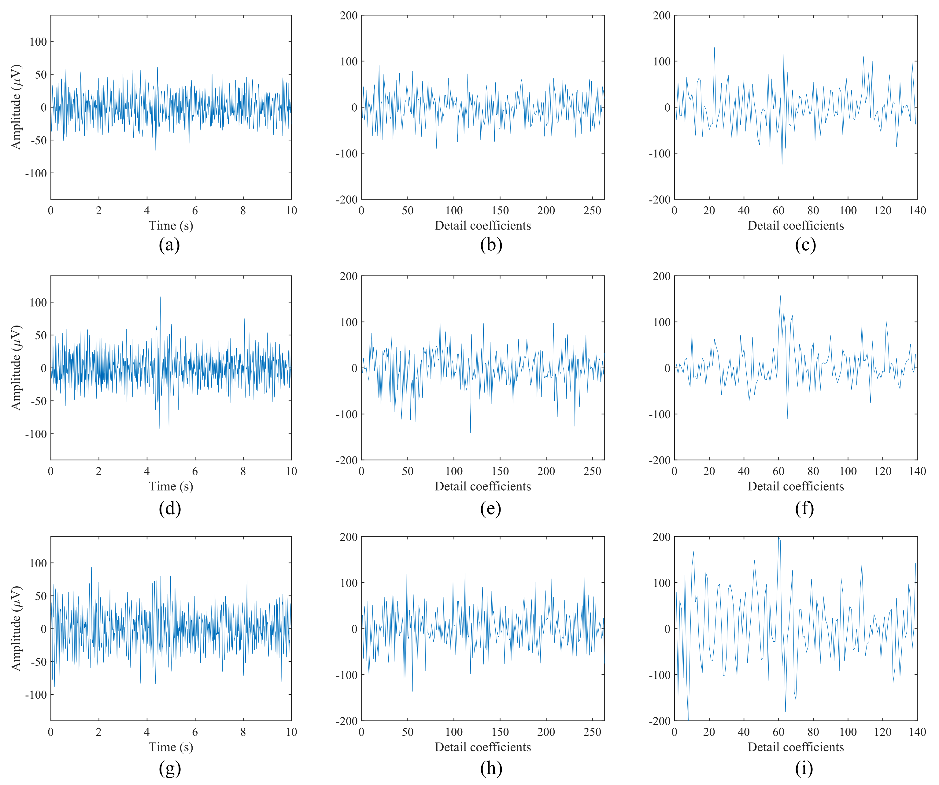
3.2. Feature Extraction and Classification
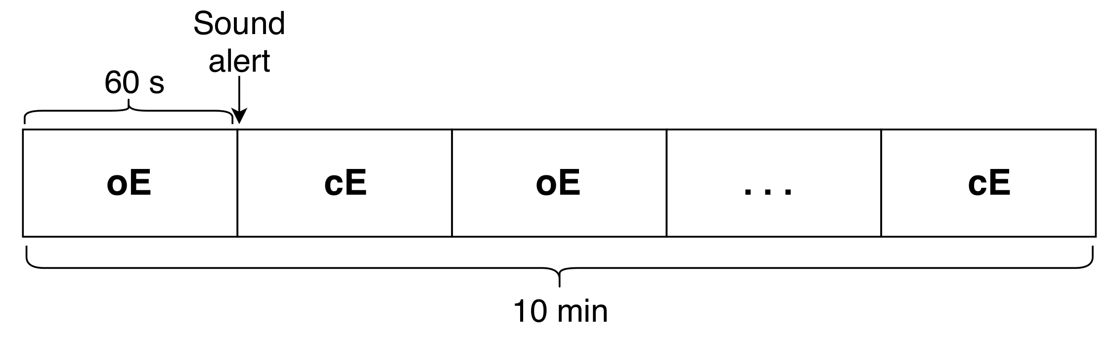
4. Materials and Methods
5. Experimental Results
5.1. Scheme 1: One Feature
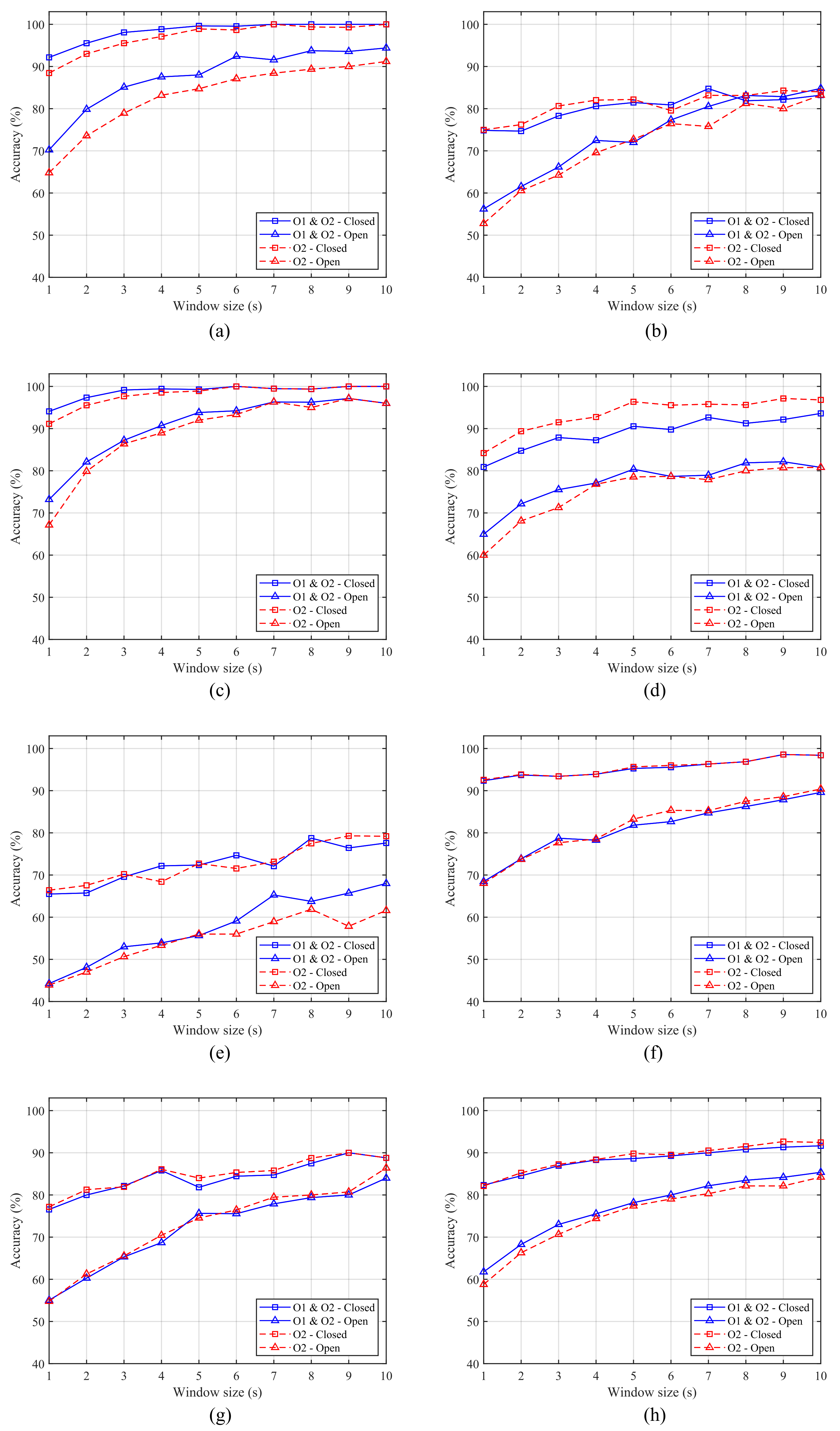
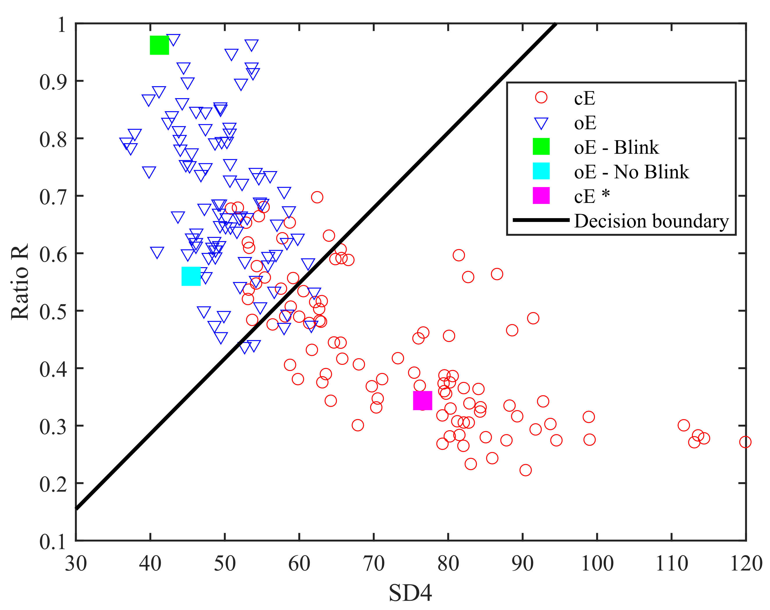
5.2. Scheme 2: Two Features
6. Discussion
7. Conclusions
Author Contributions
Funding
Institutional Review Board Statement
Informed Consent Statement
Data Availability Statement
Conflicts of Interest
Acronym
| ANN | Artificial Neural Network |
| BCI | Brain–Computer Interface |
| CAD | Computer-Aided Diagnosis |
| cE | closed eye state |
| CNN | Convolutional Neural Network |
| CWT | Continuous Wavelet Transform |
| DWT | Discrete Wavelet Transform |
| ECoG | Electrocorticography |
| EEG | Electroencephalography |
| EOG | Electrooculography |
| ERP | Event-related Potential |
| fMRI | functional Magnetic Resonance Imaging |
| FFT | Fast-Fourier Transform |
| HMI | Human–Machine Interface |
| IAL | Incremental Attribute Learning |
| LDA | Linear Discriminant Analysis |
| LR | Logistic Regression |
| MEG | Magnetoencephalography |
| MEMD | Multivariate Empirical Mode Decomposition |
| MI | Motor Imagery |
| oE | open eye state |
| PSD | Power Spectral Density |
| RNN | Recurrent Neural Network |
| SCP | Slow Cortical Potential |
| SVM | Support Vector Machine |
| VOG | Videooculography |
| WT | Wavelet Transform |
References
- Ueno, H.; Kaneda, M.; Tsukino, M. Development of drowsiness detection system. In Proceedings of the VNIS’94-1994 Vehicle Navigation and Information Systems Conference, Yokohama, Japan, 31 August–2 September 1994; pp. 15–20. [Google Scholar]
- Zhang, F.; Su, J.; Geng, L.; Xiao, Z. Driver fatigue detection based on eye state recognition. In Proceedings of the 2017 International Conference on Machine Vision and Information Technology (CMVIT), Singapore, 17–19 February 2017; pp. 105–110. [Google Scholar]
- Mandal, B.; Li, L.; Wang, G.S.; Lin, J. Towards detection of bus driver fatigue based on robust visual analysis of eye state. IEEE Trans. Intell. Transp. Syst. 2016, 18, 545–557. [Google Scholar] [CrossRef]
- Ma, J.; Zhang, Y.; Cichocki, A.; Matsuno, F. A novel EOG/EEG hybrid human–machine interface adopting eye movements and ERPs: Application to robot control. IEEE Trans. Biomed. Eng. 2015, 62, 876–889. [Google Scholar] [CrossRef]
- Estévez, P.; Held, C.; Holzmann, C.; Perez, C.; Pérez, J.; Heiss, J.; Garrido, M.; Peirano, P. Polysomnographic pattern recognition for automated classification of sleep-waking states in infants. Med. Biol. Eng. Comput. 2002, 40, 105–113. [Google Scholar] [CrossRef]
- Naderi, M.A.; Mahdavi-Nasab, H. Analysis and classification of EEG signals using spectral analysis and recurrent neural networks. In Proceedings of the 2010 17th Iranian Conference of Biomedical Engineering (ICBME), Isfahan, Iran, 3–4 November 2010; pp. 1–4. [Google Scholar]
- Wang, J.G.; Sung, E. Study on eye gaze estimation. IEEE Trans. Syst. Man Cybern. Part B Cybernet. 2002, 32, 332–350. [Google Scholar] [CrossRef]
- Kar, A.; Corcoran, P. A review and analysis of eye-gaze estimation systems, algorithms and performance evaluation methods in consumer platforms. IEEE Access 2017, 5, 16495–16519. [Google Scholar] [CrossRef]
- Krolak, A.; Strumillo, P. Vision-based eye blink monitoring system for human-computer interfacing. In Proceedings of the 2008 Conference on Human System Interactions, Krakow, Poland, 25–27 May 2008; pp. 994–998. [Google Scholar]
- Noureddin, B.; Lawrence, P.D.; Man, C. A non-contact device for tracking gaze in a human computer interface. Comput. Vis. Image Underst. 2005, 98, 52–82. [Google Scholar] [CrossRef]
- Bulling, A.; Ward, J.A.; Gellersen, H.; Tröster, G. Eye movement analysis for activity recognition using electrooculography. IEEE Trans. Pattern Anal. Mach. Intell. 2010, 33, 741–753. [Google Scholar] [CrossRef] [PubMed]
- Deng, L.Y.; Hsu, C.L.; Lin, T.C.; Tuan, J.S.; Chang, S.M. EOG-based Human–Computer Interface system development. Expert Syst. Appl. 2010, 37, 3337–3343. [Google Scholar] [CrossRef]
- Lv, Z.; Wu, X.P.; Li, M.; Zhang, D. A novel eye movement detection algorithm for EOG driven human computer interface. Pattern Recognit. Lett. 2010, 31, 1041–1047. [Google Scholar] [CrossRef]
- Barea, R.; Boquete, L.; Ortega, S.; López, E.; Rodríguez-Ascariz, J. EOG-based eye movements codification for human computer interaction. Expert Syst. Appl. 2012, 39, 2677–2683. [Google Scholar] [CrossRef]
- Laport, F.; Iglesia, D.; Dapena, A.; Castro, P.M.; Vazquez-Araujo, F.J. Proposals and Comparisons from One-Sensor EEG and EOG Human–Machine Interfaces. Sensors 2021, 21, 2220. [Google Scholar] [CrossRef]
- Laport, F.; Dapena, A.; Castro, P.M.; Vazquez-Araujo, F.J.; Iglesia, D. A Prototype of EEG System for IoT. Int. J. Neural Syst. 2020, 2050018. [Google Scholar] [CrossRef] [PubMed]
- Wang, T.; Guan, S.; Man, K.; Ting, T. Time series classification for EEG eye state identification based on incremental attribute learning. In Proceedings of the 2014 International Symposium on Computer, Consumer and Control (IS3C), Taichung, Taiwan, 10–12 June 2014; pp. 158–161. [Google Scholar] [CrossRef]
- Islalm, M.S.; Rahman, M.M.; Rahman, M.H.; Hoque, M.R.; Roonizi, A.K.; Aktaruzzaman, M. A deep learning-based multi-model ensemble method for eye state recognition from EEG. In Proceedings of the 2021 IEEE 11th Annual Computing and Communication Workshop and Conference (CCWC), Las Vegas, NV, USA, 27–30 January 2021; pp. 0819–0824. [Google Scholar]
- Reddy, T.; Behera, L. Online Eye state recognition from EEG data using Deep architectures. Proceedings of 2016 IEEE International Conference on Systems, Man, and Cybernetics (SMC), Budapest, Hungary, 9–12 October 2016; pp. 712–717. [Google Scholar] [CrossRef]
- Zhao, X.; Wang, X.; Yang, T.; Ji, S.; Wang, H.; Wang, J.; Wang, Y.; Wu, Q. Classification of sleep apnea based on EEG sub-band signal characteristics. Sci. Rep. 2021, 11, 1–11. [Google Scholar]
- Paszkiel, S. Using the Raspberry PI2 module and the brain-computer technology for controlling a mobile vehicle. In Conference on Automation; Springer: Cham, Switzerland, 2019; pp. 356–366. [Google Scholar]
- Ortiz-Rosario, A.; Adeli, H. Brain-computer interface technologies: From signal to action. Rev. Neurosci. 2013, 24, 537–552. [Google Scholar] [CrossRef] [PubMed]
- Nicolas-Alonso, L.F.; Gomez-Gil, J. Brain computer interfaces, a review. Sensors 2012, 12, 1211–1279. [Google Scholar] [CrossRef]
- Acharya, U.R.; Oh, S.L.; Hagiwara, Y.; Tan, J.H.; Adeli, H. Deep convolutional neural network for the automated detection and diagnosis of seizure using EEG signals. Comput. Biol. Med. 2018, 100, 270–278. [Google Scholar] [CrossRef]
- Yeo, M.; Li, X.; Shen, K.; Wilder-Smith, E. Can SVM be used for automatic EEG detection of drowsiness during car driving? Saf. Sci. 2009, 47, 115–124. [Google Scholar] [CrossRef]
- Kirkup, L.; Searle, A.; Craig, A.; McIsaac, P.; Moses, P. EEG-based system for rapid on-off switching without prior learning. Med. Biol. Eng. Comput. 1997, 35, 504–509. [Google Scholar] [CrossRef]
- Rösler, O.; Suendermann, D. A first step towards eye state prediction using eeg. Proc. AIHLS 2013, 1, 1–4. [Google Scholar]
- Saghafi, A.; Tsokos, C.P.; Goudarzi, M.; Farhidzadeh, H. Random eye state change detection in real-time using EEG signals. Expert Syst. Appl. 2017, 72, 42–48. [Google Scholar] [CrossRef]
- Hamilton, C.R.; Shahryari, S.; Rasheed, K.M. Eye state prediction from EEG data using boosted rotational forests. In Proceedings of the 2015 IEEE 14th International Conference on Machine Learning and Applications (ICMLA), Miami, FL, USA, 9–11 December 2015; pp. 429–432. [Google Scholar]
- Guo, H.; Burrus, C.S. Wavelet transform based fast approximate Fourier transform. In Proceedings of the 1997 IEEE International Conference on Acoustics, Speech, and Signal Processing, Munich, Germany, 21–24 April 1997; Volume 3, pp. 1973–1976. [Google Scholar]
- Bellingegni, A.D.; Gruppioni, E.; Colazzo, G.; Davalli, A.; Sacchetti, R.; Guglielmelli, E.; Zollo, L. NLR, MLP, SVM, and LDA: A comparative analysis on EMG data from people with trans-radial amputation. J. Neuroeng. Rehabil. 2017, 14, 1–16. [Google Scholar] [CrossRef] [PubMed]
- Lotte, F. A tutorial on EEG signal-processing techniques for mental-state recognition in brain–computer interfaces. In Guide to Brain-Computer Music Interfacing; Springer: Cham, Switzerland, 2014; pp. 133–161. [Google Scholar]
- Adeli, H.; Zhou, Z.; Dadmehr, N. Analysis of EEG records in an epileptic patient using wavelet transform. J. Neurosci. Methods 2003, 123, 69–87. [Google Scholar] [CrossRef]
- Samar, V.J.; Bopardikar, A.; Rao, R.; Swartz, K. Wavelet analysis of neuroelectric waveforms: A conceptual tutorial. Brain Lang. 1999, 66, 7–60. [Google Scholar] [CrossRef] [PubMed]
- Gandhi, T.; Panigrahi, B.K.; Anand, S. A comparative study of wavelet families for EEG signal classification. Neurocomputing 2011, 74, 3051–3057. [Google Scholar] [CrossRef]
- Mallat, S.G. A theory for multiresolution signal decomposition: The wavelet representation. IEEE Trans. Pattern Anal. Mach. Intell. 1989, 11, 674–693. [Google Scholar] [CrossRef]
- Subasi, A. EEG signal classification using wavelet feature extraction and a mixture of expert model. Expert Syst. Appl. 2007, 32, 1084–1093. [Google Scholar] [CrossRef]
- Quiroga, R.Q.; Sakowitz, O.; Basar, E.; Schürmann, M. Wavelet transform in the analysis of the frequency composition of evoked potentials. Brain Res. Protoc. 2001, 8, 16–24. [Google Scholar] [CrossRef]
- Quiroga, R.Q.; Garcia, H. Single-trial event-related potentials with wavelet denoising. Clin. Neurophysiol. 2003, 114, 376–390. [Google Scholar] [CrossRef]
- Hinterberger, T.; Kübler, A.; Kaiser, J.; Neumann, N.; Birbaumer, N. A brain–computer interface (BCI) for the locked-in: Comparison of different EEG classifications for the thought translation device. Clin. Neurophysiol. 2003, 114, 416–425. [Google Scholar] [CrossRef]
- Demiralp, T.; Yordanova, J.; Kolev, V.; Ademoglu, A.; Devrim, M.; Samar, V.J. Time–frequency analysis of single-sweep event-related potentials by means of fast wavelet transform. Brain Lang. 1999, 66, 129–145. [Google Scholar] [CrossRef] [PubMed]
- Zhou, J.; Meng, M.; Gao, Y.; Ma, Y.; Zhang, Q. Classification of motor imagery EEG using wavelet envelope analysis and LSTM networks. In Proceedings of the 2018 Chinese Control And Decision Conference (CCDC), Shenyang, China, 9–11 June 2018; pp. 5600–5605. [Google Scholar]
- Li, M.-A.; Wang, R.; Hao, D.-M.; Yang, J.-F. Feature extraction and classification of mental EEG for motor imagery. In Proceedings of the 2009 Fifth International Conference on Natural Computation, Tianjian, China, 14–16 August 2009; Volume 2, pp. 139–143. [Google Scholar]
- Orhan, U.; Hekim, M.; Ozer, M. EEG signals classification using the K-means clustering and a multilayer perceptron neural network model. Expert Syst. Appl. 2011, 38, 13475–13481. [Google Scholar] [CrossRef]
- Li, M.; Chen, W.; Zhang, T. Classification of epilepsy EEG signals using DWT-based envelope analysis and neural network ensemble. Biomed. Signal Process. Control 2017, 31, 357–365. [Google Scholar] [CrossRef]
- Duda, R.O.; Hart, P.E.; Stork, D.G. Pattern Classification and Scene Analysis; Wiley: New York, NY, USA, 1973; Volume 3. [Google Scholar]
- Muller, K.R.; Anderson, C.W.; Birch, G.E. Linear and nonlinear methods for brain-computer interfaces. IEEE Trans. Neural Syst. Rehabil. Eng. 2003, 11, 165–169. [Google Scholar] [CrossRef]
- Blankertz, B.; Lemm, S.; Treder, M.; Haufe, S.; Müller, K.R. Single-trial analysis and classification of ERP components—A tutorial. NeuroImage 2011, 56, 814–825. [Google Scholar] [CrossRef] [PubMed]
- Bostanov, V. BCI competition 2003-data sets Ib and IIb: Feature extraction from event-related brain potentials with the continuous wavelet transform and the t-value scalogram. IEEE Trans. Biomed. Eng. 2004, 51, 1057–1061. [Google Scholar] [CrossRef]
- Neuper, C.; Müller-Putz, G.R.; Scherer, R.; Pfurtscheller, G. Motor imagery and EEG-based control of spelling devices and neuroprostheses. Prog. Brain Res. 2006, 159, 393–409. [Google Scholar]
- Pfurtscheller, G.; Solis-Escalante, T.; Ortner, R.; Linortner, P.; Muller-Putz, G.R. Self-paced operation of an SSVEP-Based orthosis with and without an imagery-based “brain switch:” A feasibility study towards a hybrid BCI. IEEE Trans. Neural Syst. Rehabil. Eng. 2010, 18, 409–414. [Google Scholar] [CrossRef] [PubMed]
- Lotte, F.; Congedo, M.; Lécuyer, A.; Lamarche, F.; Arnaldi, B. A review of classification algorithms for EEG-based brain–computer interfaces. J. Neural Eng. 2007, 4, R1. [Google Scholar] [CrossRef] [PubMed]
- Espressif Systems (Shanghai), C. ESP32-WROOM-32 Datasheet. Available online: https://www.espressif.com/sites/default/files/documentation/esp32-wroom-32_datasheet_en.pdf (accessed on 1 April 2021).
- Jasper, H.H. The ten-twenty electrode system of the International Federation. Electroencephalogr. Clin. Neurophysiol. 1958, 10, 370–375. [Google Scholar]
- Barry, R.; Clarke, A.; Johnstone, S.; Magee, C.; Rushby, J. EEG differences between eyes-closed and eyes-open resting conditions. Clin. Neurophysiol. 2007, 118, 2765–2773. [Google Scholar] [CrossRef] [PubMed]
- La Rocca, D.; Campisi, P.; Scarano, G. EEG biometrics for individual recognition in resting state with closed eyes. In Proceedings of the 2012 BIOSIG-Proceedings of the International Conference of Biometrics Special Interest Group (BIOSIG), Darmstadt, Germany, 6–7 September 2012; pp. 1–12. [Google Scholar]
- Gale, A.; Dunkin, N.; Coles, M. Variation in visual input and the occipital EEG. Psychon. Sci. 1969, 14, 262–263. [Google Scholar] [CrossRef]
- Ogino, M.; Mitsukura, Y. Portable drowsiness detection through use of a prefrontal single-channel electroencephalogram. Sensors 2018, 18, 4477. [Google Scholar] [CrossRef] [PubMed]
- Al-Qazzaz, N.K.; Hamid Bin Mohd Ali, S.; Ahmad, S.A.; Islam, M.S.; Escudero, J. Selection of mother wavelet functions for multi-channel EEG signal analysis during a working memory task. Sensors 2015, 15, 29015–29035. [Google Scholar] [CrossRef] [PubMed]


| Levels | Frequency Band (Hz) | EEG Rhythm | Decomposition Level |
|---|---|---|---|
| D1 | 50–100 | Noise | 1 |
| D2 | 25–50 | Beta-Gamma | 2 |
| D3 | 12.50–25 | Beta | 3 |
| D4 | 6.25–12.50 | Theta-Alpha | 4 |
| A4 | 0–6.25 | Delta-Theta | 4 |
| Wavelet | Filter Length | Closed | Open | ||
|---|---|---|---|---|---|
| O1 and O2 (%) | O2 (%) | O1 and O2 (%) | O2 (%) | ||
| db2 | 4 | 86.29 | 86.97 | 74.63 | 72.11 |
| db4 | 8 | 88.23 | 89.83 | 81.03 | 79.43 |
| db8 | 16 | 92.46 | 92.69 | 85.14 | 84.00 |
| coif1 | 6 | 86.97 | 87.89 | 76.34 | 75.54 |
| coif4 | 24 | 91.66 | 92.46 | 85.37 | 84.23 |
| haar | 2 | 86.74 | 89.03 | 73.14 | 71.09 |
| sym2 | 4 | 86.29 | 86.97 | 74.63 | 72.11 |
| sym4 | 8 | 90.17 | 91.31 | 81.49 | 80.00 |
| sym10 | 20 | 94.63 | 92.46 | 84.46 | 82.29 |
| Subject | Closed | Open | ||
|---|---|---|---|---|
| O1 and O2 (%) | O2 (%) | O1 and O2 (%) | O2 (%) | |
| 1 | 100.00 | 100.00 | 94.40 | 91.20 |
| 2 | 83.20 | 84.00 | 84.80 | 83.20 |
| 3 | 100.00 | 100.00 | 96.00 | 96.00 |
| 4 | 93.60 | 96.80 | 80.80 | 80.80 |
| 5 | 77.60 | 79.20 | 68.00 | 61.60 |
| 6 | 98.40 | 98.40 | 89.60 | 90.40 |
| 7 | 88.80 | 88.80 | 84.00 | 86.40 |
| Mean | 91.66 | 92.46 | 85.37 | 84.23 |
| Wavelet | Filter Length | Closed | Open | ||
|---|---|---|---|---|---|
| O1 and O2 (%) | O2 (%) | O1 and O2 (%) | O2 (%) | ||
| db2 | 4 | 93.49 | 91.31 | 98.29 | 96.57 |
| db4 | 8 | 94.06 | 92.80 | 98.86 | 97.71 |
| db8 | 16 | 94.40 | 93.83 | 99.31 | 97.60 |
| coif1 | 6 | 93.71 | 92.91 | 98.17 | 96.80 |
| coif4 | 24 | 94.40 | 93.71 | 99.09 | 97.49 |
| haar | 2 | 93.37 | 91.54 | 97.94 | 96.11 |
| sym2 | 4 | 93.49 | 91.31 | 98.29 | 96.57 |
| sym4 | 8 | 93.94 | 93.03 | 98.06 | 97.03 |
| sym10 | 20 | 94.40 | 93.03 | 98.63 | 97.37 |
| Subject | Closed | Open | ||
|---|---|---|---|---|
| O1 and O2 (%) | O2 (%) | O1 and O2 (%) | O2 (%) | |
| 1 | 100.00 | 100.00 | 100.00 | 100.00 |
| 2 | 84.00 | 80.00 | 96.00 | 89.60 |
| 3 | 100.00 | 100.00 | 100.00 | 96.00 |
| 4 | 95.20 | 95.20 | 100.00 | 100.00 |
| 5 | 93.60 | 95.20 | 100.00 | 100.00 |
| 6 | 92.00 | 91.20 | 100.00 | 98.40 |
| 7 | 96.00 | 95.20 | 99.20 | 99.20 |
| Mean | 94.40 | 93.83 | 99.31 | 97.60 |
Publisher’s Note: MDPI stays neutral with regard to jurisdictional claims in published maps and institutional affiliations. |
© 2021 by the authors. Licensee MDPI, Basel, Switzerland. This article is an open access article distributed under the terms and conditions of the Creative Commons Attribution (CC BY) license (https://creativecommons.org/licenses/by/4.0/).
Share and Cite
Laport, F.; Castro, P.M.; Dapena, A.; Vazquez-Araujo, F.J.; Fresnedo, O. Eye State Identification Based on Discrete Wavelet Transforms. Appl. Sci. 2021, 11, 5051. https://doi.org/10.3390/app11115051
Laport F, Castro PM, Dapena A, Vazquez-Araujo FJ, Fresnedo O. Eye State Identification Based on Discrete Wavelet Transforms. Applied Sciences. 2021; 11(11):5051. https://doi.org/10.3390/app11115051
Chicago/Turabian StyleLaport, Francisco, Paula M. Castro, Adriana Dapena, Francisco J. Vazquez-Araujo, and Oscar Fresnedo. 2021. "Eye State Identification Based on Discrete Wavelet Transforms" Applied Sciences 11, no. 11: 5051. https://doi.org/10.3390/app11115051
APA StyleLaport, F., Castro, P. M., Dapena, A., Vazquez-Araujo, F. J., & Fresnedo, O. (2021). Eye State Identification Based on Discrete Wavelet Transforms. Applied Sciences, 11(11), 5051. https://doi.org/10.3390/app11115051