A Deep Learning Model to Forecast Solar Irradiance Using a Sky Camera

Abstract

Solar irradiance fluctuates mainly due to clouds. A sky camera offers images with high temporal and spatial resolutions for a specific solar photovoltaic plant. The cloud cover from sky images is suitable for forecasting local fluctuations of solar irradiance and thereby solar power. Because no study applied deep learning for forecasting cloud cover using sky images, this study attempted to apply the long short-term memory algorithm in deep learning. Cloud cover data were collected by image processing of sky images and used for developing the deep learning model to forecast cloud cover 10 min ahead. The forecasted cloud cover data were plugged into solar radiation models as input in order to predict global horizontal irradiance. The forecasted results were grouped into three categories based on sky conditions: clear sky, partly cloudy, and overcast sky. By comparison with solar irradiance measurement at a ground station, the proposed model was evaluated. The proposed model outperformed the persistence model under high variability of solar irradiance such as partly cloudy days with relative root mean square differences for 10-min-ahead forecasting are 25.10% and 39.95%, respectively. Eventually, this study demonstrated that deep learning can forecast the cloud cover from sky images and thereby can be useful for forecasting solar irradiance under high variability.

1. Introduction

Clouds have a serious impact on photovoltaic (PV) power production. By limiting the levels of solar irradiance reaching the PV, the clouds can contribute to the high variability of PV power output. Therefore, it is necessary to monitor cloud formation and obtain information about clouds in order to be able to prepare backup energy sources that will cover any reductions in energy output. Cloud information is applied in weather analyses and meteorological data; also, it is used for energy applications such as solar irradiance and PV power estimation. Furthermore, cloud information, such as cloud cover and cloud motion, has frequently been examined as a source of renewable energy. Chow et al. [1] used a sky camera installed in California to develop a method for intra-hour cloud motion and to forecast global horizontal irradiance (GHI). Kim et al. [2] used sky images to retrieve cloud cover and validated these images through human observations to estimate solar irradiance. Lothon et al. [3] investigated an algorithm to estimate the cloud cover from sky images.

Cloud information is a key input variable for solar irradiance forecasting, which is a critical issue to manage uncontrollable production of PV power. In general, many methods are able to forecast solar irradiance, and these methods are grouped according to the forecast horizon. For long-term forecast horizons, numerical weather prediction that relies on the numerical solution of governing equations in meteorological sciences is most useful. Because predictions can be made up to 15 days in advance, such long-term forecast horizon helps operation optimization and market participation. On the other hand, sky images and satellite images are used for forecasting solar irradiance in the short-term forecast horizon. These methods are able to forecast solar irradiance several minutes to several hours in advance. This short-term forecasting is useful in the anticipation of ramp events caused by variations in solar irradiance. Compared to satellite images, sky images offer more detailed cloud information with higher spatial resolution. Therefore, the solar irradiance forecasting based on sky images is appropriate for management of a specific PV system, in spite of shorter time horizon.

In general, information about clouds, especially for cloud cover data, is collected through human observations, and the World Meteorological Organization provides the rules for the registration of cloud cover. Observers estimate the cloud cover in oktas or tenths, in which the sky is divided into 8 or 10 regions and the regions that are covered by clouds are evaluated. However, the accuracy of this traditional method is deemed unsatisfactory: it provides low temporal and spatial resolutions, and errors can be introduced through the subjective nature of observers’ judgments. Hence, a hemispherical sky camera is an alternative solution that can be used to address some of these problems. The camera gathers images at high frequency during the hours of daylight.

The fast evolution of low-cost hemispherical sky cameras has been preferred due to their application in gathering cloud information [4], and they have become very popular in the fields of solar energy and cloud motion detection. The sky camera is able to produce cloud cover information by image processing from pixel distribution. The data are calculated based on an algorithm that applies the red, green, and blue (RGB) channels of an image and combines them with an adaptive threshold in order to distinguish the cloud and sky pixels. Besides, this data can be combined with physical models to estimate solar irradiance. For example, Kim et al. [5] used cloud cover to estimate solar irradiance in South Korea using the cloud cover radiation model. This model is a regression-type model that was developed by Kasten et al. [6] to estimate GHI on an hourly basis. Furthermore, some researchers have also used sky images to forecast solar irradiance in short-term forecast horizons. Caldas et al. [7] forecasted GHI using sky images and real-time GHI measurements. They applied the cloud correlation model (CCM) to these images to predict GHI up to 10 min in advance. These results indicate that the proposed model was able to predict GHI in a very short-term forecast horizon under high variability of solar irradiance.

So far, the GHI forecasting using sky images was calculated using conventional methods, such as CCM and cloud motion vector (CMV). They estimated the cloud motion by calculating the motion of the pixels on images. However, these methods did not provide good accuracy because the cloud motion is not linear and hard to predict. Meanwhile, deep learning, which is the subpart of artificial intelligence (AI), has been increasingly used in solar irradiance and PV power forecasting [8,9,10,11]. Various deep learning models, such as recurrent neural network (RNN), long short-term memory (LSTM), gated recurrent unit (GRU), and deep belief network (DBN), provide high accuracy in forecasting solar irradiance for both short-term and long-term forecast horizons. Nevertheless, no studies applied deep learning models to forecast the solar irradiance using cloud cover data obtained from sky images.

In this study, we proposed a method to estimate solar irradiance in high variability of solar irradiance such as partly cloudy days. The proposed method combines the cloud cover obtained from sky images, the deep learning model to forecast the cloud cover ten minutes ahead, and the physical model to estimate GHI with the forecasted cloud cover. 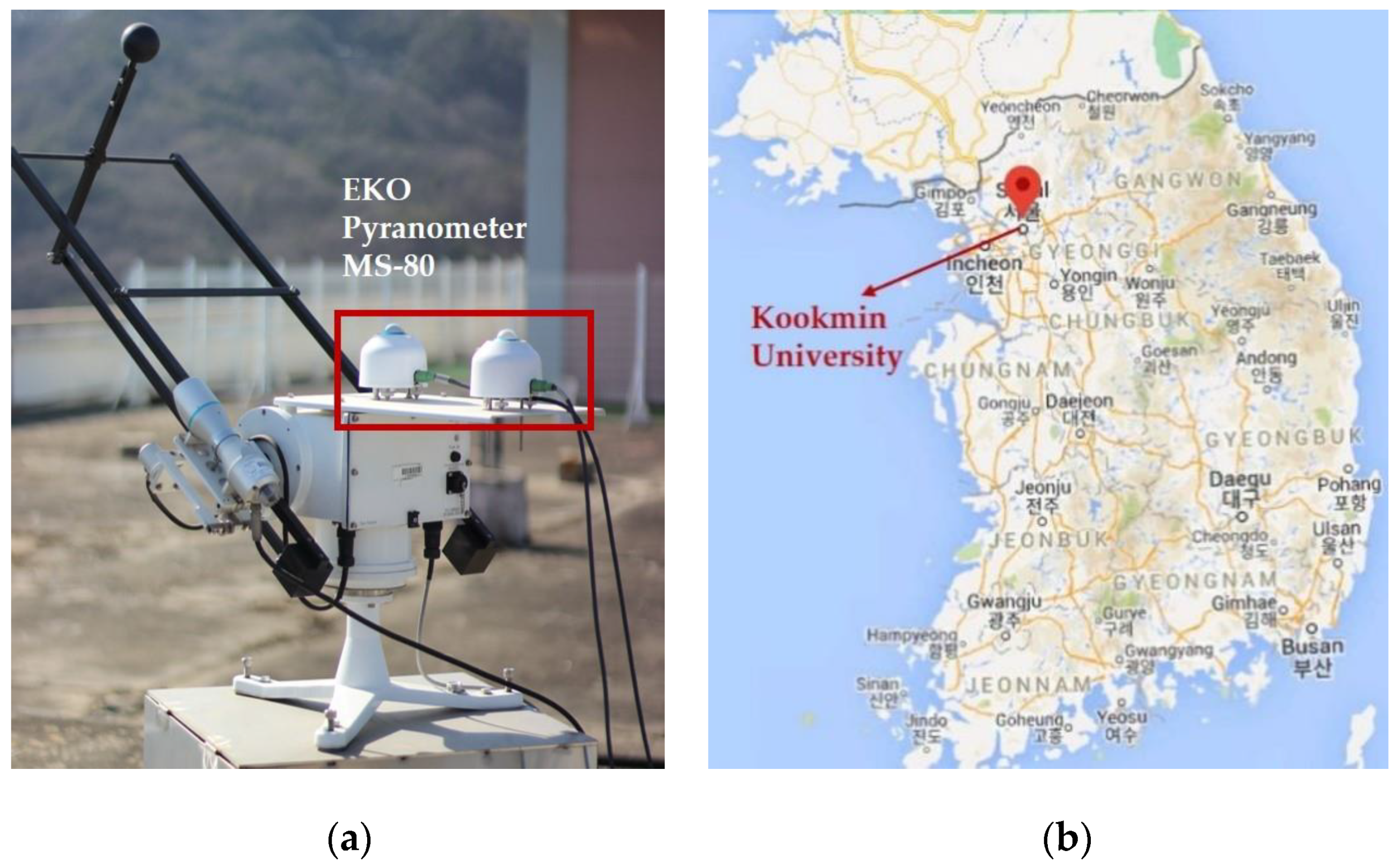The LSTM was selected out of deep learning algorithms because it is recommendable for predicting time-series data compared with other deep learning models [8]. The forecasting was conducted for clear, cloudy, and overcast days on a minute basis and validated by the comparison with GHI measurement at a ground station in Seoul, South Korea. Because no study used the deep learning model to forecast the cloud cover from sky images, this study will investigate its applicability.

2. Data and Instrument

Two instruments have been utilized in this study: a sky camera used to capture the sky image and a pyranometer used to measure the GHI. The instruments were set up on the rooftop at Kookmin University in Seoul, South Korea (latitude: 37.61200° N, longitude: 126.99770° E).

2.1. Sky Image

Sky images were obtained using a Total Sky Camera J1006 as shown in Figure 1a, which captured sky images every minute. A fish-eye lens as the angle projection was then attached to the camera, which provides a 180° field of view in the horizontal direction. The camera system is based on a digital camera with a maximum resolution of 2272 × 1704 pixels, and the images were stored locally in a computer at the Kookmin University. The camera system contains large-capacity silica gel drying cartridges to keep the inside of the instrument free of moisture. A ventilation unit was also applied to prevent the deposit of dust and dew on the optical system and to protect the sky camera against thermal heating effects.

The sky images captured through the fish-eye lens were calibrated using a checkerboard calibration pattern to correct the fish-eye image. First, pictures were taken of the checkerboard in different positions and orientations, as shown in Figure 1b. Then, the MATLAB toolbox was used to detect the image and world points on the checkerboard as the calibration parameters. The image and checkerboard points were applied as the input for the image calibration in converting all the images to flat images.

2.2. Solar Irradiance

Solar irradiance measurement revolves around three components, that is, global horizontal irradiance (GHI), diffuse horizontal irradiance (DHI), and direct normal irradiance (DNI). The GHI is the total solar irradiance that reaches the earth’s surface, which is the combination of DNI and DHI. The GHI can be measured using a pyranometer that has been designed to receive solar irradiance from all directions. In this study, the GHI was measured using a EKO pyranometer MS-80 in Kookmin University (see Figure 2a,b). The pyranometer was then installed with ventilation units that cover the dome of the pyranometer to protect it from dew and frost during the morning and to reduce the effects of raindrops and dust. The pyranometer has a response time of less than 0.5 s with an approximate sensitivity of 10 µV/Wm⁻² and collects the GHI in 1-min, 10-min, 1-hr, and 1-day intervals. The pyranometer was calibrated following the ISO 9060:2018 standard.

2.3. Classification of Sky Conditions

In order to forecast solar irradiance using sky images during a variety of sky conditions, the 25 days from May to August in July 2020 were selected. These days provided all-sky conditions based on the clear-sky index and variability. Thereafter, days have been grouped according to the mean of the clear-sky index and clear-sky index variability, which is calculated using the following equation:

$${\mu }_{kt}=\frac{1}{n}{\displaystyle \sum _{i=1}^n\frac{GH{I}_m{}_{}}{GH{I}_c}}$$

(1)

$${\delta }_{kt}=Std\{k{t}_{t-1}-k{t}_t\}$$

(2)

where $kt$ is the clear-sky index, ${\mu }_{kt}$ is the mean of the clear-sky index, $GH{I}_m$ is the GHI measurement, $GH{I}_c$ is the clear-sky GHI, and ${\delta }_{kt}$ is the clear sky index variability. Statistics from the clear-sky index can be used to determine the sky conditions. The clear-sky index estimates the atmospheric attenuation due to the clouds by measuring the ratio of the surface solar radiation to the solar radiation received under a clear sky. In this study, the days have been grouped into three categories [12] as shown in Figure 3: clear-sky day $({\mu }_{kt}>0.65)$ and $({\delta }_{kt}<0.03)$, partly cloudy day $(0.3\le {\mu }_{kt}\le 0.65)$ and $({\delta }_{kt}>0.10)$, and overcast day $({\mu }_{kt}<0.3)$ and $({\delta }_{kt}<0.03)$. Figure 4 compares the GHI measurement variability in all sky conditions for three representative days. It illustrates the small variation in GHI for clear and overcast days from 9:00 a.m. to 5:00 p.m. On the other hand, the partly cloudy day presents the high GHI variability with the maximum and the minimum values of GHI are 956.0 Wm⁻² and 184.0 Wm⁻², respectively.

3. Methods

The method to forecast solar irradiance, which is comprised of the two steps, is presented in this section. In the first step, the cloud cover is calculated from sky images, and then the future cloud cover is predict using LSTM. In the second step, the GHI is forecasted by applying the predicted cloud cover for the solar radiation model as the input data.

3.1. Cloud Cover Algorithm

To include further details of the cloud cover retrieval, we have created a simple flow chart of the algorithm used to detect the cloud and sky pixels on images, as shown in Figure 5. This flow chart outlines the process of obtaining the cloud cover from sky images by using the distribution of the pixel values in images. The first step is to collect the sky images from the sky camera. These images are converted into a one-channel image in order to improve the contrast and to reduce the noise of the image by applying the RBR method; this method was proposed by Shield et al. [13] and is able to successfully detect the cloud and sky pixels in an image. Mathematically, the RBR method is defined as the ratio of the red and blue channels of an image with the pixel value ranging from 0 to 255. It should be noted that the value of the blue channel is increased by 1 if it equals 0 to avoid dividing by 0 [14].

After that, the threshold value is applied to the one-channel image to distinguish the clouds from the sky. We calculated the value using the Otsu thresholding method that Nobuyaski Otsu proposed back in 1979 [15]. This method was chosen on account of its flexibility and robustness in identifying the cloud and sky pixels. Another advantage of this method is the simple process involved in determining the threshold values: since the calculation requires one-dimensional intensity data, the other parameters, such as the shape or geometric components of an object, do not affect the accuracy of the threshold value.

It is worth noting that the basic concept in thresholding is to segment an image based on the difference between the pixel value. Therefore, a fixed threshold value cannot be applied to all-sky images because the brightness in sky images differs on account of the ever-changing position of the sun. To address these problems, the threshold value is adapted to all images, and this makes the value different in each image.

Finally, the cloud cover was calculated using the ratio of cloud pixels to total pixels based on the percentage of the cloud pixels in the binary image. The measurement of cloud cover is reported in the number of parts of the sky covered by clouds. The sky can be split into 8 (oktas) or 10 (tenths) parts representing the amount of cloud in a particular sky. It should also be noted that cloud cover does not describe the cloud thickness and that it only refers to the amount of the sky covered by clouds in a particular location.

3.2. Solar Radiation Model

The solar radiation model has been used to estimate GHI using various input data. One of the solar radiation models that uses cloud cover as the input data is the Kasten model [6]. This regression-type model estimates GHI by using a correlation between the cloud cover and clear-sky irradiance. In this model, the cloud cover was divided into 9 classes, where 0 refers to a clear sky and 8 an overcast sky. This model has been widely used in different locations, but some researchers had to modify the coefficients in order to obtain results in their location. In this specific location in Seoul, the coefficients were obtained from research conducted by Yoo et al. [16]. The GHI is calculated using this formula:

$$GHI=GH{I}_c\times (1-A\times {(0.125\times CC)}^B)$$

(3)

$$GH{I}_c=C\times \sin (\alpha )-D$$

(4)

where $CC$ is the cloud cover, $GH{I}_c$ is the solar irradiance on clear sky condition, $\alpha$ is solar elevation, A = 0.75, B = 2.6, C = 963, and D =106. However, the specific value does not reach the GHI under overcast sky conditions, since the minimum value for an overcast sky is a quarter of clear-sky irradiance. Therefore, we proposed a new model by modifying the coefficient in Kasten’s model and the clear sky irradiance model. The coefficients to calculate the GHI for each model are presented in

Table 1. The coefficients to estimate global horizontal irradiance (GHI) for each model.

Model	A	B
Kasten	0.75	3.4
Yoo [16]	0.75	2.6
Proposed	0.95	3.4

.

Many clear-sky irradiance models have been made available to calculate the solar irradiance under clear sky conditions, and each of these models requires different parameters as the input. For example, Dazhi et al. [17] calculated clear-sky irradiance in combination with the solar zenith angle and the eccentricity of the earth. Antonanzas-Torres et al. [18] estimated solar irradiance based on commonly measured variables, such as temperature, rainfall, and humidity. Yang et al. [19] proposed a model to calculate solar irradiance based on ozone absorption, water vapor absorption, permanent gas absorption, aerosol extinction, and Rayleigh scattering. In this work, we used the Ineichen clear-sky model after modification by Reno et al. [20], as this model affords good accuracy and fairly easy to execute. The equations to obtain the clear-sky irradiance obtained from are expressed as follows:

$$GH{I}_c=c_{g1}\times I_o\times \cos ({\theta }_z)\times \exp (-c_{g2}\times AM\times (f_{h1}+f_{h2}\times (T_L-1)))\times \exp (0.01\times A{M}^{1.8})$$

(5)

$$AM=\frac{1}{\cos ({\theta }_z)+0.50572\times {(96.07995-{\theta }_z)}^{-1.6364}}$$

(6)

$$f_{h1}=\exp (-d/8000)$$

(7)

$$f_{h2}=\exp (-d/1250)$$

(8)

$$c_{g1}=5.09\times {10}^{-5}\cdot d+0.868$$

(9)

$$c_{g2}=3.92\times {10}^{-5}\cdot d+0.0387$$

(10)

where $I_o$ is extraterrestrial normal incident irradiance, ${\theta }_z$ is solar zenith, $AM$ is air mass, $T_L$ is linked turbidity factor, and $d$ is the ground elevation expressed in meters.

Here, the linked turbidity refers to the optical thickness of the atmosphere due to the presence of gaseous water vapor and the absorption and scattering by the aerosol [21]. It expresses the transparency of the sky or cloudless atmosphere. In a case where the sky is perfectly blue (clean), the $T_L$ value is close to 1. However, if the sky has high water vapor and the color is closer to white, the $T_L$ becomes larger. The air mass refers to the relative path length of the direct solar beam through the atmosphere, and it describes the ratio of the distance traveled by solar radiation in reaching the atmosphere to the distance of the sun directly overhead. Note, in this solar irradiance model, the air mass is dependent solely on the so-lar zenith.

3.3. Deep Learning Model

In this study, we used LSTM as a deep learning model to forecast the cloud cover up to several minutes ahead. LSTM was chosen as it provides satisfactory results in handling time series data. Rajagukguk et al. [7] identified that this model performs better than other deep learning models, such as RNN and GRU. Furthermore, this deep learning model demonstrates good performance in solar irradiance forecasting in both short-term and long-term forecast horizons. LSTM was developed to overcome the problems with vanishing and explosion gradients that often occur in other deep learning models. For instance, in the case of the RNN, when these problems occurred in the learning process, the learning performance failed to increase [22].

The LSTM model was proposed by Hochreiter and Scmidhuber to adapt to the long-term dependence on the information [23]. The unit, as has been illustrated in Figure 6, consists of forget gate, input gate, output gate, and cell state. For simplicity’s sake, the structure can be formulated as follows:

$$f_t=\sigma \left(W_f\times x_t+U_f\times h_{t-1}+b_f\right)$$

(11)

$$i_t=\sigma \left(W_i\times x_t+U_i\times h_{t-1}+b_i\right)$$

(12)

$$S_t=\tanh \left(W_c\times x_t+U_c\times h_{t-1}+b_c\right)$$

(13)

$$C_t=i_t\odot S_t+f_t\odot C_{t-1}$$

(14)

$$o_t=\sigma {\left(W_o\times x_t+U_o\times h_{t-1}+V_o\times C_t+b_o\right)}^{ }$$

(15)

$$h_t=o_t\odot \tanh \left(C_t\right)$$

(16)

where $f_t$ is the forget gate, $i$ is the input gate, $o_t$ is the output gate, $x{ }_t$ is input data, $b$ is bias, $W$,$U$,$V$ are weight matrices, $h_{t }$ is the value of memory cell, $S_{ t}$ is candidate state of the memory cell,$\tanh$ and $\sigma$ are the activation functions, and $C{ }_t$ is the state of the memory cell.

In Equations (11), (12) and (15), the sigmoid function is used to calculate the amount of information that passes through the gate with values from 0 to 1. The candidate state of the memory cell in Equation (13) contains the $\tanh$ function that makes the value ranging from −1 to 1 in order to calculate the new information. The input and forgot gates in Equation (14) are operated with the Hadamard product $(\odot )$ to calculate the state memory of the cell. The final output of the memory cell in Equation (16) was obtained after multiplying with the output gate.

A total of 12,000 images were processed to obtain minutely cloud cover information in this study. These calculated data provided the input for LSTM to forecast the future cloud cover. To illustrate the model design, the details of these hyperparameters are listed in

Table 2. The hyperparameters used in designing the LSTM model.

Hyperparameter	Searching for Optimal Value	Optimal Value
Epoch	[50,100,200,300,400,500]	300
Activation function	ReLU	ReLU
Batch size	[64,128,256]	128
Optimization	Adam	Adam
Learning rate	0.001	0.001

.

The optimum hyperparameters such as epochs, batch size, learning rate, optimization algorithm, and activation functions for deep learning models depend on the datasets. The epochs describe the number of complete passes (forward and backward) through the neural network. The batch size denotes the number of training examples in one pass (forward and backward). The learning rate controls the weight in a neural network with reference to loss gradient. The optimization algorithm is used to find the attributes, such as determining the weights neural network to reduce the losses. Along with this structure, this LSTM model is also equipped with an activation function known as a rectified linear unit (ReLU). ReLu is a non-linear function that oppresses a value below 0 to become exactly 0 but still inherits some linear property for cases above 0. Because this function has a linear characteristic, it can easily train by a deep network of neurons and also solve a case of gradient problem by ignoring the negative values. It should be noted that there is no fixed value in deep learning models to explain the optimum design for each model because the networks inside deep learning models are trained iteratively. Therefore, the best way to determine the optimal hyperparameter was to use errors during validation and training to assess the algorithm’s accuracy.

3.4. Evaluation Metric

In order to validate the performance of forecasting, various common evaluation metrics have been used to calculate the accuracy of the model, including mean bias difference (MBD), root mean square difference (RMSD), relative root means square difference (rRMSD), and relative mean bias difference (rMBD). We prefer to use differences rather than errors as the measurement data by nature include uncertainty; hence, the true values are unknown [24]. The evaluation metrics are given in the following equations:

$$MBD=\frac{1}{n}{\displaystyle \sum _{i=1}^n\left(P_e-P_m\right)}$$

(17)

$$RMSD=\sqrt{\frac{1}{n}{\displaystyle \sum _{i=1}^n{\left(P_e-P_m\right)}^2}}$$

(18)

$$rMBD=\frac{\frac{1}{n}{\displaystyle \sum _{i=1}^n\left(P_e-P_m\right)}}{\frac{1}{n}{\displaystyle \sum _{i=1}^n{P}_m}}$$

(19)

$$rRMSD=\frac{\sqrt{\frac{1}{n}{\displaystyle \sum _{i=1}^n{\left(P_e-P_m\right)}^2}}}{\frac{1}{n}{\displaystyle \sum _{i=1}^n{P}_m}}\cdot 100$$

(20)

where $P_e$ is the estimated values at each time, $P_m$ is the measured values at each time, and $n$ is the number of sample data for the period.

The RMSD explains the deviation from the measurement and it always generates a positive value. This value measures how close the prediction is to the measurement; thus, a smaller value is deemed better. The MBD shows the average bias of the prediction, and it also provides the long-term performance of the model [25], where the positive and negative values represent overprediction and underprediction, respectively. Furthermore, in cases where the data vary with location and time scale, relative metrics such as rRMSD and rMBD are more useful, as they provide the percentage difference.

4. Results and Discussion

This section provides the results from both the RBR model used to obtain the cloud cover and the deep learning model used to forecast solar irradiance. The RBR method detects the presence of clouds by considering the ratio of the red channels to blue channels in a color image. These one-channel images combined with the threshold values were able to distinguish cloud pixels from the background. In the sky images, the cloud and sky pixels were detected as white and black colors and were further transformed from the original image into the binary image to facilitate the identification of cloud and sky pixels. However, in some cases, errors occurred when the cloud pixel was almost the same as the sky pixel. In addition, if the clouds are extremely thin, the pixels are lower than the threshold value, and they are not detected as clouds. Hence, it is essential to determine an accurate threshold value to lessen the occurrence of such classification errors.

In order to understand the correlation between cloud cover and the clear-sky index, the distribution of the daily calculated cover data is presented in Figure 7, which illustrates the variation of mean cloud cover for each day. To investigate the results, the mean clear-sky index has been converted into an opposite value on account of the differences in the definition of sky conditions in relation to cloud cover and the clear-sky index; for example, in referring to cloud cover, a value of 0 is a clear-sky condition, while in the clear-sky index, a value of 0 refers to an overcast sky. The correlation between the cloud cover and the clear-sky index is worth mentioning because it shows similar trends, which indicates that the method provides satisfactory results in obtaining the cloud cover from sky images.

In forecasting results, the forecast cloud cover using the LSTM model is converted into GHI data using the correlation cloud cover and clear-sky irradiance as described in Equation (3). The results for the minutes forecasting were compared with the GHI measurement in terms of evaluation metrics. The summary of solar irradiance forecasting is grouped in three categories based on sky conditions: partly cloudy, clear, and overcast days. The proposed model by modifying the coefficient in Kasten’s model outperformed the Yoo model and the persistence model for partly cloudy days as shown in

Table 3. Evaluation metrics of forecast performance between the proposed, the Yoo, and the persistence models for partly cloudy days.

Forecast Horizon	Proposed				Yoo [16]				Persistence
	RMSD	MBD	rMSD	rMBD	RMSD	MBD	rMSD	rMBD	RMSD	MBD	rMSD	rMBD
(minute)	(Wm−2)	(Wm−2)	(%)	(%)	(Wm−2)	(Wm−2)	(%)	(%)	(Wm−2)	(Wm−2)	(%)	(%)
1	137.00	7.58	18.05	1.66	144.12	−50.72	18.98	−11.14	219.70	−10.13	28.94	3.81
2	143.67	12.76	20.08	2.97	153.20	−60.91	21.41	−14.19	343.17	35.52	47.96	6.70
3	154.72	−6.57	20.92	−1.48	165.26	−78.41	22.35	−17.67	379.92	11.76	51.38	6.95
4	167.50	−30.19	21.31	−6.40	173.02	−92.77	22.01	−19.67	319.28	−59.65	40.61	5.17
5	166.49	−14.75	21.68	−3.20	172.28	−78.49	22.44	−17.04	296.78	−43.61	38.65	5.03
6	173.84	17.77	23.15	3.94	181.78	−39.79	24.21	−8.83	310.31	−35.94	41.33	5.50
7	178.33	−16.36	23.49	−3.59	185.04	−84.15	24.37	−18.47	169.01	−12.96	22.26	2.93
8	190.83	−20.86	26.03	−4.74	201.44	−100.89	27.47	−22.93	170.84	7.13	23.30	3.18
9	187.02	−31.19	25.49	−7.09	205.31	−115.21	27.99	−26.17	299.60	15.42	40.84	5.57
10	199.75	−60.65	25.10	−12.70	214.97	−131.53	27.01	−27.54	317.94	−43.28	39.95	5.02

. After 10 min forecasting, the RMSD for the proposed, the Yoo, and the persistence models are 199.75 Wm⁻², 214.97 Wm⁻², and 317.94 Wm⁻², respectively. For reference, another forecasting model by Caldas et al. [7], which used the cross-correlation method (CCM) in all-sky imaging, attained an RMSD of 251 Wm⁻² for partly cloudy days in forecasting solar irradiance up to 10 min in advance.

The results for clear days and overcast days are shown in

Table 4. Root mean square difference (RMSD) between the proposed, the Yoo, and the persistence models for clear days and overcast days.

Forecast Horizon	Clear Days			Overcast Days
	Proposed	Yoo [16]	Persistence	Proposed	Yoo [16]	Persistence
(minute)	(Wm−2)	(Wm−2)	(Wm−2)	(Wm−2)	(Wm−2)	(Wm−2)
1	20.59	35.44	6.20	17.74	74.32	2.52
2	31.59	39.15	7.79	16.73	90.66	3.66
3	37.80	31.78	14.04	18.17	98.26	4.67
4	45.70	41.40	20.92	19.41	99.86	9.43
5	45.56	57.56	28.26	19.34	104.51	6.64
6	29.69	59.68	56.24	20.20	138.79	5.48
7	34.76	54.05	41.74	20.46	119.06	8.30
8	34.15	53.76	38.28	17.33	158.65	7.26
9	40.27	58.20	49.26	15.60	155.47	6.48
10	43.08	63.74	52.49	17.37	169.86	9.98

. The results indicate that under clear day conditions the proposed model outperforms the persistence and the Yoo models for forecast horizon more than 5 min. The RMSD in 10 min forecasting for the proposed, the Yoo, and the persistence models are 43.08 Wm⁻², 63.74 Wm⁻², and 52.49 Wm⁻², respectively. However, the information was different on overcast days. In this case, the smallest error by the persistence model, the RMSD of 9.98 Wm⁻² in 10 min ahead of forecasting, demonstrated that the persistence model performed well under the overcast condition. The proposed and the Yoo models provide the RMSD of 17.37 Wm⁻² and 169.86 Wm⁻², respectively. The result in these overcast days was not surprising since the value of solar irradiance does not change significantly. The experiment by Caldas et al. [7] also reported that the persistence model has better performance than their proposed model for overcast day conditions, with an RMSD of 110 Wm⁻² for 10 min ahead forecast horizon.

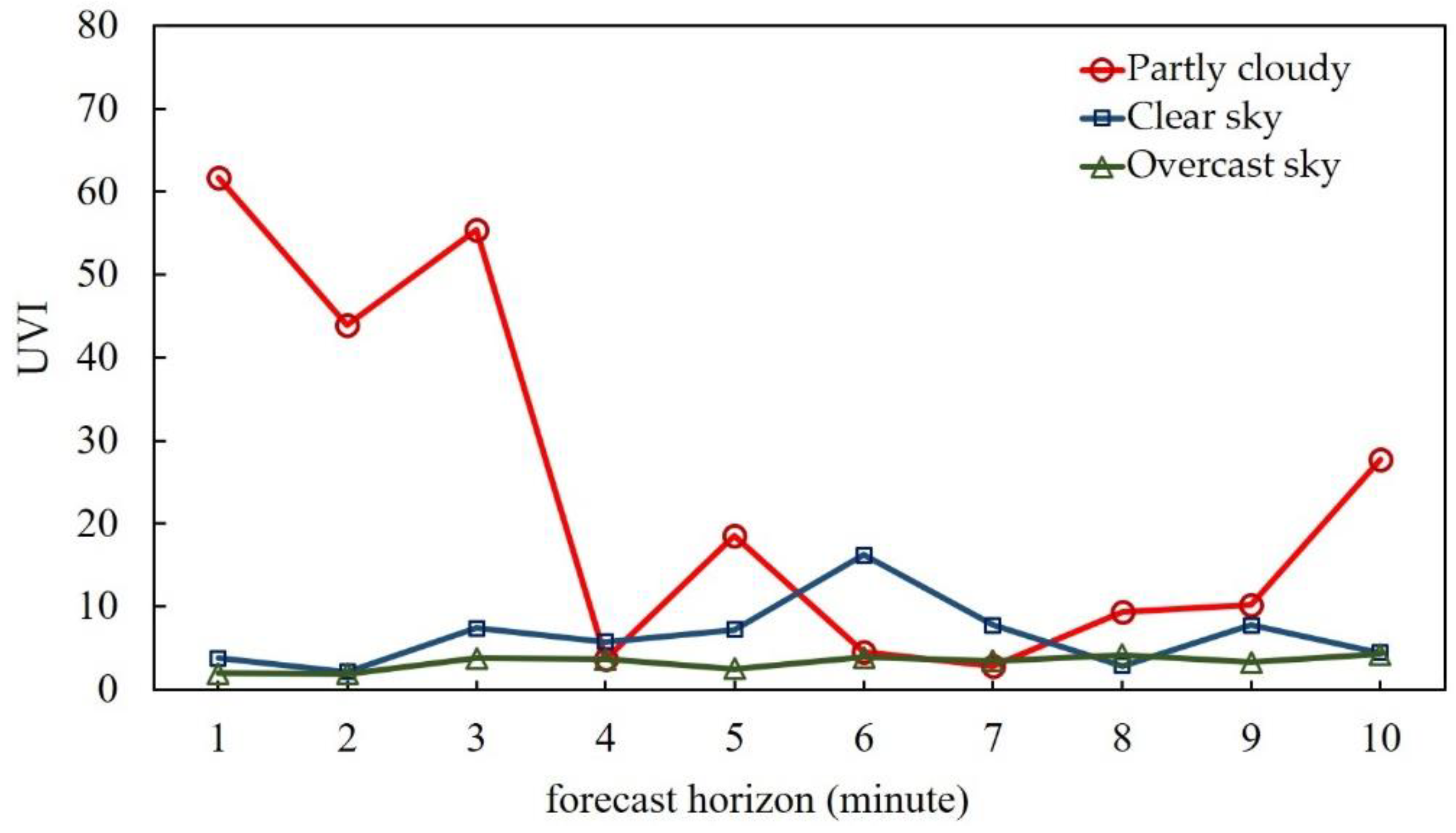
To further analyze the variability of the solar irradiance under different sky conditions, the metric that indicates the variability of solar irradiance is presented in Figure 8. The metric was calculated using the universal variability index (UVI) to quantify the variation of solar irradiance under clear, partly cloudy, and overcast days by comparing the measured irradiance and calculated clear-sky irradiance. As expected, the small variations in clear and overcast days resulted in the values of UVI close to one. However, the UVI for partly cloudy days does not remain constant anymore due to the high variability of solar irradiance. It shows the high variability index with the value ranging from 2.68 to 61.16.

The performance of forecast models significantly differs by solar irradiance variability. Figure 9 shows the mean RMSD and the mean UVI of 10-min-ahead forecast results under different sky conditions. It clearly explains that the proposed model remarkably outperformed the persistence model in partly cloudy days with the mean UVI > 20. On the other hand, when the mean UVI < 5, the forecast performance of the proposed model is comparable to that of the persistence model. In overcast days, the proposed model is slightly less accurate than the persistence model. Probably, the reason is that the solar radiation model is less accurate under overcast sky conditions.

5. Conclusions

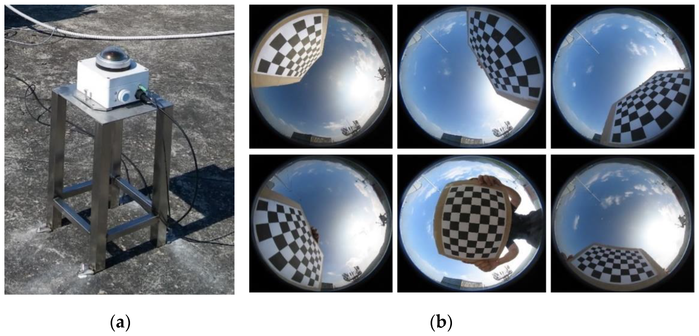
In this study, a model to forecast solar irradiance from sky images was proposed and evaluated. The images recorded using a sky camera were designed to capture a hemispherical image each minute. Image processing using the RBR method was used to improve the quality of the image in detecting the cloud pixels in the image. The LSTM, as a deep learning model, was applied to forecast the cloud cover for several minutes ahead. Then, the physical model was used to estimate the GHI by using the forecasted cloud cover.

When the sky is partly cloudy, i.e., the UVI is larger than 20, the proposed model is able to forecast GHI for 10 min in advance with RMSD, rMSD, MBD, and rMBD values of 199.75 Wm⁻², 25.1%, −60.65 Wm⁻², and −12.70%. These evaluation metrics demonstrate that the proposed model has a better performance than the Yoo and the persistence models. On the other hand, for clear and overcast sky conditions when the UVI is smaller than 5, performances of the proposed and the persistence models are comparable.