Article

Short-Term Load Forecasting Using an Attended Sequential Encoder-Stacked Decoder Model with Online Training

by
Sylwia Henselmeyer
1,* and
Marcin Grzegorzek
2
1
Siemens AG, Humboldtstr. 59, 90459 Nuremberg, Germany
2
Institute of Medical Informatics, University of Lubeck, 23562 Lubeck, Germany
*
Author to whom correspondence should be addressed.
Appl. Sci. 2021, 11(11), 4927; https://doi.org/10.3390/app11114927
Submission received: 2 May 2021 / Revised: 22 May 2021 / Accepted: 24 May 2021 / Published: 27 May 2021
(This article belongs to the Special Issue Advanced Methods of Power Load Forecasting)

Abstract

:
The paper presents a new approach for the prediction of load active power 24 h ahead using an attended sequential encoder and stacked decoder model with Long Short-Term Memory cells. The load data are owned by the New York Independent System Operator (NYISO) and is dated from the years 2014–2017. Due to dynamics in the load patterns, multiple short pieces of training on pre-filtered data are executed in combination with the transfer learning concept. The evaluation is done by direct comparison with the results of the NYISO forecast and additionally under consideration of several benchmark methods. The results in terms of the Mean Absolute Percentage Error range from 1.5% for the highly loaded New York City zone to 3% for the Mohawk Valley zone with rather small load consumption. The execution time of a day ahead forecast including the training on a personal computer without GPU accounts to 10 s on average.

1. Introduction

Load forecasts are substantial in several areas of power network operation independently of the voltage level. With the increasing number of renewables and thus more volatility and dynamics in the network, the task of load forecasting becomes even more important. Errors in forecasts have direct financial consequences on the utilities and in the long-term on their customers. They also may lead to an inexcusable waste of the green power in the case it has to be curtailed due to network congestions.
Load forecasts are usually subdivided into three categories concerning the length of the prediction horizon:
  • short-term: from a few minutes until one week ahead
  • mid-term: from one week until one year ahead
  • long-term: from one year until several years ahead
Short-term load forecasts are used to guarantee a safe and optimal real-time network operation (prevention of network violations, unit commitment, and economic dispatch). Mid-term load forecasts are more important for planning maintenance tasks, load redispatch, and securing a balanced load and generation. Long-term forecasts are mainly relevant for network reassembling and expansion.
In the area of short-term load forecasting, two basic groups of methods have been established, i.e., methods based on statistics and so-called intelligent approaches [1]. Statistical methods are usually easy to implement and provide quick results. A standard method from the group of statistical approaches is multiple regression [2,3]. It can cope with changes in the load data due to trending or seasonal impacts and it can include in the forecast model different kinds of independent variables such as weather and calendar or the load data from previous time instances. To guarantee good prediction results, training data from at least one year before the forecast begins is required. Other well-established statistical forecast methods are General Exponential Smoothing with inclusion of seasonality (Holt-Winters) [4] and autoregressive integrated moving average (ARIMA) [5,6] and combination of ARIMA and Artificial Neural Networks [7]. They can consider influences resulting from changing trends, seasonal differences and irregularities in load data and work well with a limited amount of training samples. However, external variables such as weather cannot be included in their models.
Statistical methods expect an exact mathematical model of load and its influencing factors. Parameters of the model are estimated from the historical data samples. Fuzzy logic approaches from the class of intelligent techniques get along with a high-level model specification expressed with the “IF”-“THEN” statements [8,9]. Another group of intelligent approaches are Artificial Neural Networks (ANNs) [10,11]. They require the definition of the neural network to be used and pairs of input and output data. Since they can approximate any function hidden in the data, they are very well suited for tasks where an explicit model description is too complicated or the underlying function undergoes frequent changes which are difficult to capture such as for example in load forecasting in electric power networks with a high number of renewable sources.
With the advances in the research and the application of neural networks, the classical multi-perceptron networks (MPN) [12,13] are more and more replaced by recurrent or convolutional networks or combinations of these. Recurrent neural networks can represent time dependency by sharing the hidden layers of subsequent time steps. From this category, especially Gated Recurrent Units (GRU) [14] and the even more powerful Long Short-Term Memory (LSTM) networks [15] and their combined usage with convolutional networks [11,16], the Genetic Algorithm (GA) and Particle Swarm Optimization (PSO) for hyperparameter search [17,18] shall be mentioned. Different than simple recurrent networks, these architectures do not experience the so-called gradient vanishing or exploding problems [19] and are to some extent able to memorize longer time series sequences and provide therefore superior results over MPLs or simple recurrent architectures.
Lately, originated from the research on machine translation problems also encoder-decoder architectures are being applied to the load forecast problem. Ref. [20] used it for the prediction of the load heat. The basic idea is to encode the information required for the forecast execution before passing it to the actual forecast model. This decoupling is crucial for machine translation and shows however good effects while applied to time series prediction problems. An extension of this architecture is the incorporation of the attention mechanism as introduced by Bahdanau in [21] in the area of natural language processing. The attention approach allows for choosing those encoder states which may be most influential for the prediction of the next decoder state. Ref. [22] applied the attention model with Bahdanau attention [21] to the load forecasting using Vanilla, GRU, and LSTM cells achieving in general superior results over non attended sequence to sequence models. In [23] multi-headed attention together with a seasonal decomposition and trend adjustment is used. Ref. [24] uses the classic combination of attended encoder-decoder model with GRU cells as proposed by [21]. Additionally, to simplify the choice of the hyperparameters the Bayesian optimization is applied.
The goal of the presented approach is the development of an improved attended encoder-decoder architecture and its application to the problem of short-term load forecasting considering the increasing number of renewable sources. Before passing to the model, the inputs of the encoder and decoder are weighted using a one-dimensional convolutional neural network. This operation allows for filtering out features that have a temporarily lower correlation with the load power to predict. Additionally, a novel online training based on its core of the concept of transfer learning is presented [25,26,27].
The scientific contribution of the presented paper is therefore an improved attended sequential encoder-stacked decoder model applied to the problem of short-term load prediction with:
  • a novel and simplified definition of the attention scoring function
  • a novel online training procedure for sequence data on the base of transfer learning. This training procedure is especially important in the field of very dynamically changing load patterns.
  • a high accuracy achieved on real data provided by NYISO
  • an evaluation with different methods including linear regression, Hidden Markov Models and different recurrent neural network architectures
In the next Section 2.1, the data set is discussed along with the feature selection. In Section 2.2 and Section 2.3 the definitions of a recurrent network, an LSTM, encoder-decoder model and attention are compiled. Using these definitions, the method is described in Section 2.4. The results obtained by the proposed approach are evaluated together with the results available from NYISO and with additional benchmark methods in Section 3. The conclusions can be found in the final Section 4.

2. Materials and Methods

2.1. Data Used

The data used for training and evaluation of the approach is owned by the New York Independent System Operator (NYISO) and can be freely accessed [28]. It has been already used in [29] and therefore it will be possible to compare the results of both approaches. NYISO’s data consists of integrated hourly load forecasts and corresponding measurements of active load power. Moreover, load information, NYISO additionally offers time series representing the price for power delivery, losses, and congestion in USD and forecasts of ambient and wet bulb temperature in Fahrenheit produced by different weather stations.
The NYISO data set is almost complete (with a few missing inputs) for all eleven zones. Because it includes also the forecast results of the utility, it is very adequate for research purposes.
The training, test, and evaluation data used in the presented approach contain load, temperature, and wet bulb time series from the years 2013 until 2015, 2016, and 2017 respectively. The decision to not consider price information was motivated by the very low correlation between load and price data. More details related to the data set are in [29].
The most strongly correlated features are the load power and the ambient temperature. However, this relationship differs concerning the season as described in [29] and varies strongly depending on the temperature range. Figure 1 shows daily load curves for subsequent working days in May 2017 in the New York City data. Remarkable are strongly different daily peak values causing different load curve shapes. The peak values increase from 6 [GW] on 15.05.17, over 6.5 [GW] on 16.05.17 until 8 [GW] on 17.05.17.
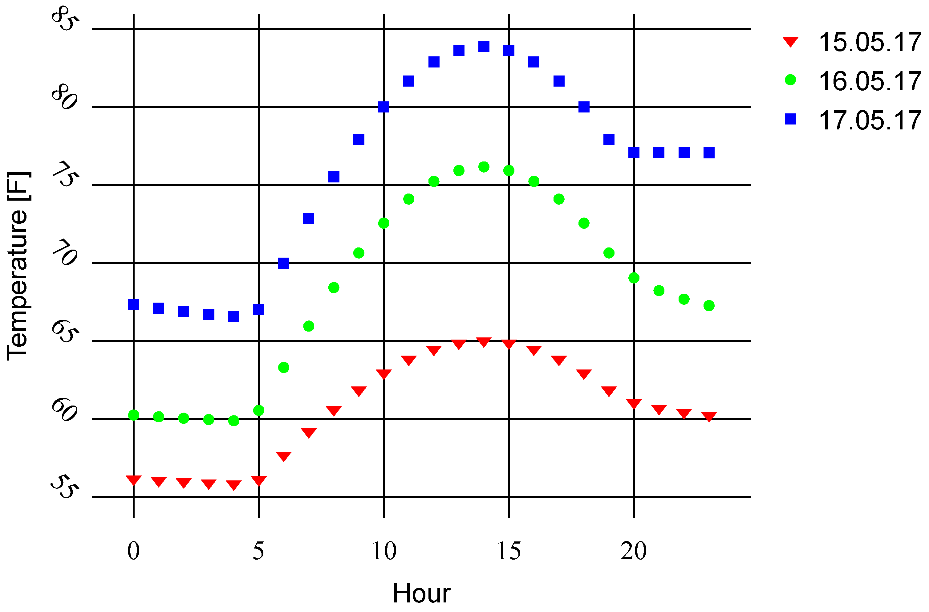
The corresponding daily temperature curves shown in Figure 2 document the same order of increase of the peak values from 15.05.17 until 17.05.17 indicating a relationship between both variables.
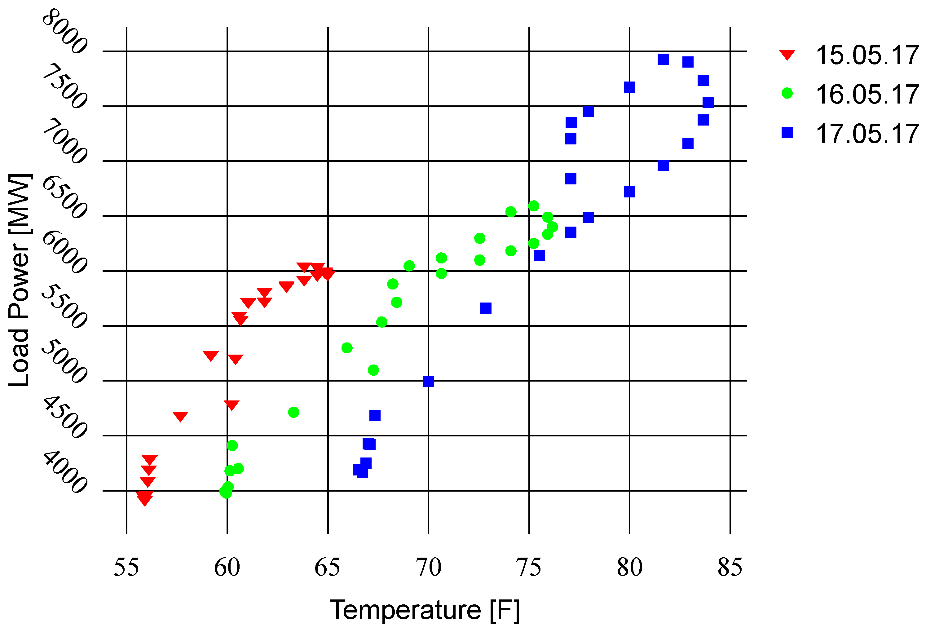
Figure 3 shows this relationship which is non-linear and differs strongly for each day discussed. Because of this fact, the conclusion is self-evident, which is that the commonly used sliding window approach for the choice of the training data such as for example in [24] cannot be successful here. Instead, the choice of the training is based on similar-day approach [12,30]. The reason is that following days can have strongly differing load patterns due to changing weather conditions. Therefore, the similar day approach seems to be superior.
Before the training, time series with missing entries or outlier values are excluded from the data set. The training, test, and evaluation are executed on the z-score normalized data according to Equation (1) with μ the feature mean and σ feature standard deviation. For the calculation of the accuracy of the method, the data are however transformed back to the original value space.
z i = x i μ σ .

2.2. Recurrent Network with Long Short-Term Memory Cell

Recurrent networks are a group of neural networks which is developed to support the dealing of the temporal aspects in the data [31]. This is achieved while conditioning the hidden state from a time instance t not only on the input for time t but also on the hidden state at the time instance t 1 . In simple recurrent networks also called Elman networks, three matrices are shared over all time instances. A matrix W which stores weights connecting input x t and hidden state h t , a matrix U containing the weights between the hidden states of subsequent time instances and the matrix V which transforms the hidden states to the network output. Accordingly, the hidden state h t is obtained from the application of an activation function g on the weighted input and previous hidden state (2). The network output y t is calculated using an activation function f on the weighted hidden state h t as specified in (3).
h t = g ( U h t 1 + W x t )
y t = f ( V h t )
One of the problems of Elman networks is that information inserted early time instances may become lost at later ones. A solution to that problem is Long Short-Term Memory (LSTM) cells which can filter out information not required at further time steps and keep the one that may be needed later on. This is achieved by adding a recurrent context layer and several weight matrices and gates in combination with the usage of the sigmoid activation function as presented in Figure 4.
A Long Short-Term Memory cell consists of the forget gate (4), the input gate (5), the cell update gate (6) and the output gate (7). The context C t is obtained from the sum of the pointwise multiplication (⊗) of the context from time instance t 1 and the forget gate and the cell update gate and the input gate (8). The output for the time instance y t is calculated through the pointwise multiplication of the context at time instance t and the output gate (9).
f t = σ ( U f x t + W f h t 1 )
i t = σ ( U i x t + W i h t 1 )
C ^ t = t a n h ( U g x t + W g h t 1 )
o t = σ ( U o x t + W o h t 1 )
C t = σ ( C t 1 f t + C ^ t i t )
h t = y t = t a n h ( C t o t )

2.3. Encoder-Decoder and Attention

The encoder-decoder architecture developed in the domain of machine translation is constructed of two separated mostly recurrent networks called the encoder and the decoder. Figure 5 shows an example of such architecture using LSTM networks. The goal of the encoder network is to provide a compressed representation of the input sequence which is then passed to the decoder as the initial state. The decoder creates the output sequence subsequently one by one using the output from the preceding time instance as the input at the following one. Because of this, the encoder-decoder architecture is very well suited for time series problems.
The encoder-decoder model is very powerful but has however one significant limitation. While encoding the input sequence, often the information relevant for the creation of a correctly decoded output becomes lost. This is solved using the attention mechanism. At its core, the attention concept evaluates the similarity score between each encoder output and the currently produced decoder output. The goal is to draw attention to those encoder sequence parts which are most significant for the current decoder output. In [21] first the similarity score between each encoder state stored in h j and the previous decoder output s t 1 is calculated (10). The softmax function is applied to the similarity coefficients (11). From that, the context vector is calculated (12) which is then concatenated with the decoder hidden state of the time instance t 1 .
e i j = v a T t a n h ( W a s t 1 + U a h j )
α i j = e x p ( e i j ) k = 1 T x e x p ( e i k )
c i = j = 1 T x α i j h j
Using these equations, the attention is drawn to those parts of the encoder which are most significant while decoding the ith element of the sequence.

2.4. Application of the Attended Encoder-Decoder to the Short-Term Load Forecasting

2.4.1. Training Data

As mentioned in Section 2.1, the training data consists not of n recent days like it is established through the sliding window approach. It contains n most similar days to the day under forecast. The similarity of two days d a y i and d a y j is expressed by the Equation (13) and it considers the weighted Euclidean distance d ( d a y i , d a y j ) between the features measured at that days. Most similar days have the smallest distance between the respective features.
d ( d a y i , d a y j ) = k = 0 N w k f i , k f j , k 2
The weight allows for larger differences in features that are wider spread and for smaller differences in those which are contained within a narrow interval.
w k = 1 | f k m a x f k m i n |
The feature set used for filtering of the most similar days consists of:
  • daily minimum ambient temperature and wet bulb
  • daily maximum ambient temperature and wet bulb
  • daily minimum next day ambient temperature and wet bulb
  • load power one hour before the intended forecast start before forecast start
  • the type of the day (working day, weekend or holiday)
  • the length of the day
  • the type of the day concerning the ambient temperature (hot, cold, regular day)
To predict the hourly load curve for the next day, data of 96 most similar training days is used.

2.4.2. Application of Encoder-Decoder Architecture

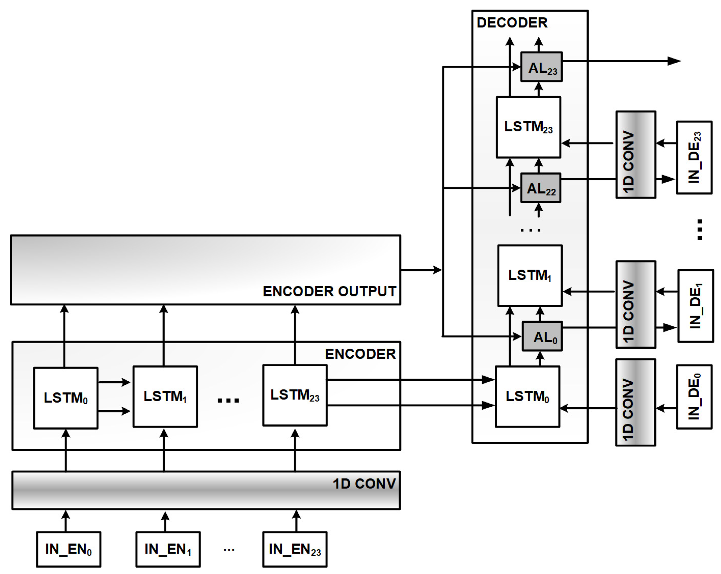
The encoder accepts inputs for the last 24 h before the forecast day as shown in Figure 6. The decoder is fed with hourly chunks of the time-series data related to hourly ambient temperature, hourly wet bulb, the type of the day, etc. at the forecast day and the output of the decoder cell at the previous time instance (except the first decoded time step).
Each encoder and decoder input consists of:
  • the hour h,
  • the load power from hour h 1 (for decoder the previous predicted value),
  • the ambient temperature and wet bulb from hour h,
  • the day of the week (0–6),
  • the type of the day concerning the temperature (hot, cold, regular),
  • the type of the day concerning holiday or working day,
  • the length of the day
The usage of the load power alone as encoder input as done in [24] increased the prediction error, therefore it was not applied here. The encoder and decoder input is processed with a 1D convolutional filter to account for changing relevance of the input data depending on temperature and day type.
The encoder is used as a sequential model, the decoder as a stacked architecture as shown in Figure 6. During the test, it turned out that it is beneficial concerning the forecast error to apply a separate convolution and attention layer for each decoded instance. This might be related to the varying correlation between the encoder outputs and the decoder output at time t.

2.4.3. Attention Score Function

During the development of the algorithm, a simplified score function showed slightly better results. In Equation (15), the absolute difference between the encoder output h of the dimension N and the last decoder output s t 1 adjusted to the dimension of the encoder is calculated. Afterwards the softmax function is applied twice (16) and (17). The first time, to map the differences obtained from Equation (15) to the interval [ 0 , 1 ] . The second time, to assign small differences between the decoder and encoder output to the upper part of the interval [ 0 , 1 ] and larger differences to the lower part (17). The final context vector is obtained in (18) as a sum over the time dimension. The decoder state for which the attention is applied is concatenated with the context vector. Finally, a dense layer is used to adjust the size of the concatenated vector to the output produced by the LSTM cell.
e i j = | h s t 1 × N |
α i j = e x p ( e i j ) k = 1 T x e x p ( e i k )
β i j = e x p ( 1 α i j ) k = 1 T x e x p ( 1 α i k )
c i = j = 1 T x β i j h j
In this formulation, only one weight matrix is required instead of three matrices as specified in (10). The forecast error while using both formulations of attention is however similar.

2.4.4. Online Training—A Piecewise Learning of the Underlying Function

The standard training approach as applied for example in natural language processing consists of a choice of representative training and validation data. The goal is to learn the approximation of the underlying function in one training procedure and to use the model for a longer period. The validation data are used to control the progress and the quality of the training. Such holistic training procedures can be quite a time-consuming one depending on the complexity of the function to be learned expressed in the network architecture and the number of training data required. Additional problems arise if there is not enough representative training data available or there is a sudden change in the underlying function which is not captured in the chosen training data. In load forecasting, holidays and abnormal days (very cold or very hot) are usually underrepresented and there is no simple method to create artificial data without prior knowledge of the underlying function. Due to the increasing number of renewables and prosumers, load patterns are subject to further unexpected changes. Therefore, there must be a possibility to train the network fast with a limited amount of training data.
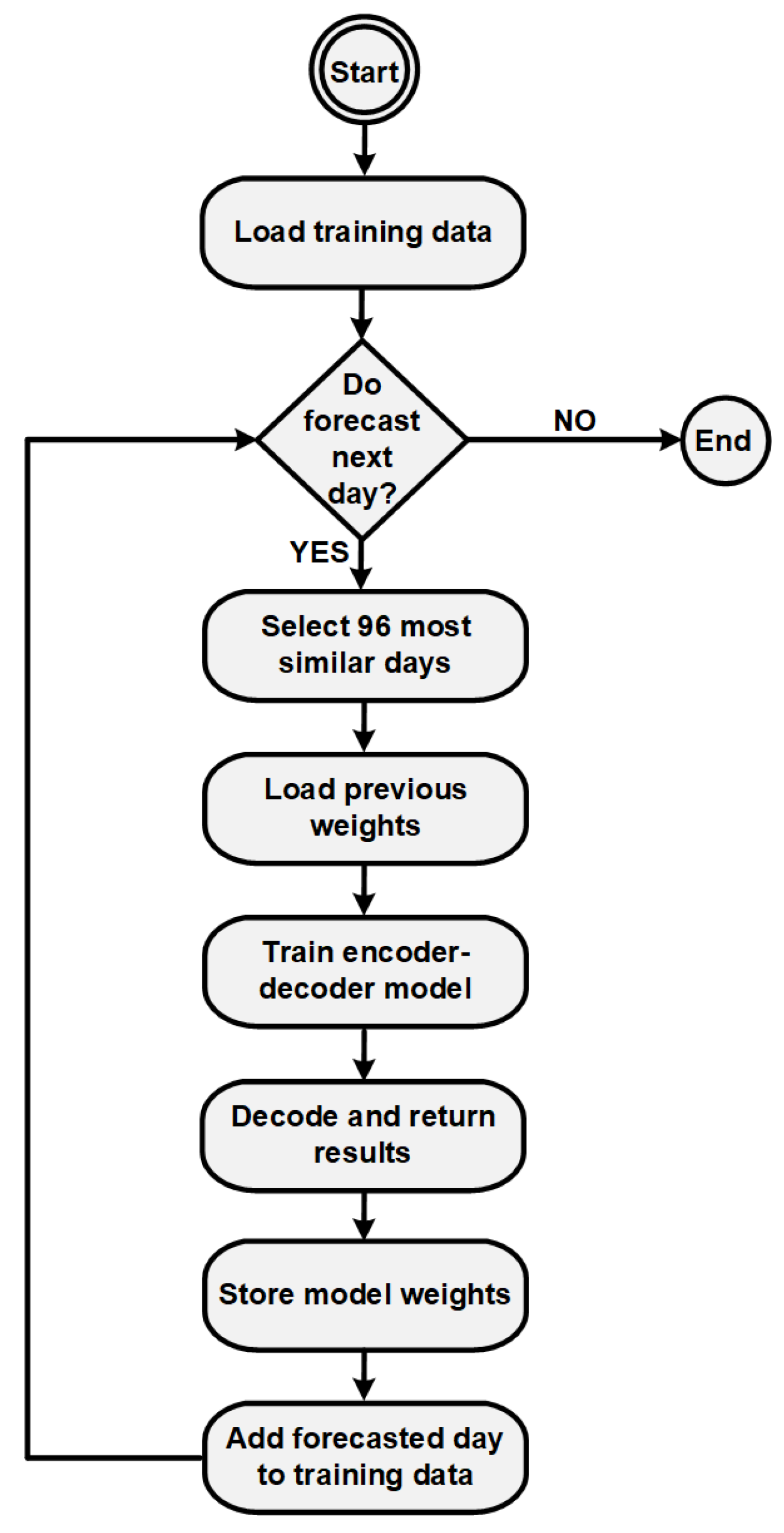
In the presented approach, transfer learning [25,26] in combination with online training is being used to cope with time-consuming training procedure, the insufficient amount of training data especially for weekends and hot days, and changing load patterns. Figure 7 shows an overview of the training and inference procedure.
The preprocessed training data are loaded. If the forecast for the next day’s load power shall be executed, the most similar days are picked. If available, the weights from the previous day are loaded into the model. The encoder-decoder model is trained for 50 epochs in one batch using the ADAM optimizer. Each training data related to the day d a y j is weighted according to the Euclidean distance to the time series under prediction d a y i as calculated by Equation (13) shown in (19).
w j t r a i n = 100 | m a x ( d ( d a y i , d a y 1 : n ) ) d ( d a y i , d a y j ) ) m a x ( d ( d a y i , d a y 1 : n ) ) |
No validation data are used but an early stopping criterion is applied if the value of the loss function falls below the threshold of 0.0001 . The approximated piece of the underlying function follows the data in the training data set. The prediction results are decoded and returned. The weights are stored so that they can be reused as a starting point for the next training. The data of the forecasted day is added to the training data set. Using this approach, the training time is distributed in small chunks on each day to be forecasted. Additionally, the most recent data can be easily included in the training procedure capturing the most recent changes in the load pattern.

3. Results

The evaluation of the approach has been executed on the data from 2017 and it includes all NYISO zones. Table 1 compiles the name, the abbreviation, and the average load for each zone. The power consumption is varying because the zones differ concerning the size of the area, the number of residents, and the type of housing (cities, villages, rural areas). New York City is the zone with the highest number of residents. The power consumption for that area is accordingly high. Mohawk Valley on the other side, has a relatively large area, a small number of residents and therefore a significantly smaller load [28].
The results obtained from the sequential encoder-stacked decoder with attention (SESDA) are evaluated together with the results of three other methods. First of them is the Hidden Markov Model approach from [29]. The Hidden Markov Models used there were created online using the data directly without any training procedure. Additionally, the results of the NYISO are taken into account [28,32]. The third benchmark is a linear regression method from [3] and is named Tao’s Vanilla Benchmark. It already has served as a benchmark for the GEFCom2012 load forecast competition and was under the first 25% best results of that competition [33].
The prediction error is measured by the Mean Absolute Percentage Error (MAPE) which is specified by Equation (20), with M as measured value and P as the predicted value.
M A P E = 100 % n t = 1 n M t P t M t
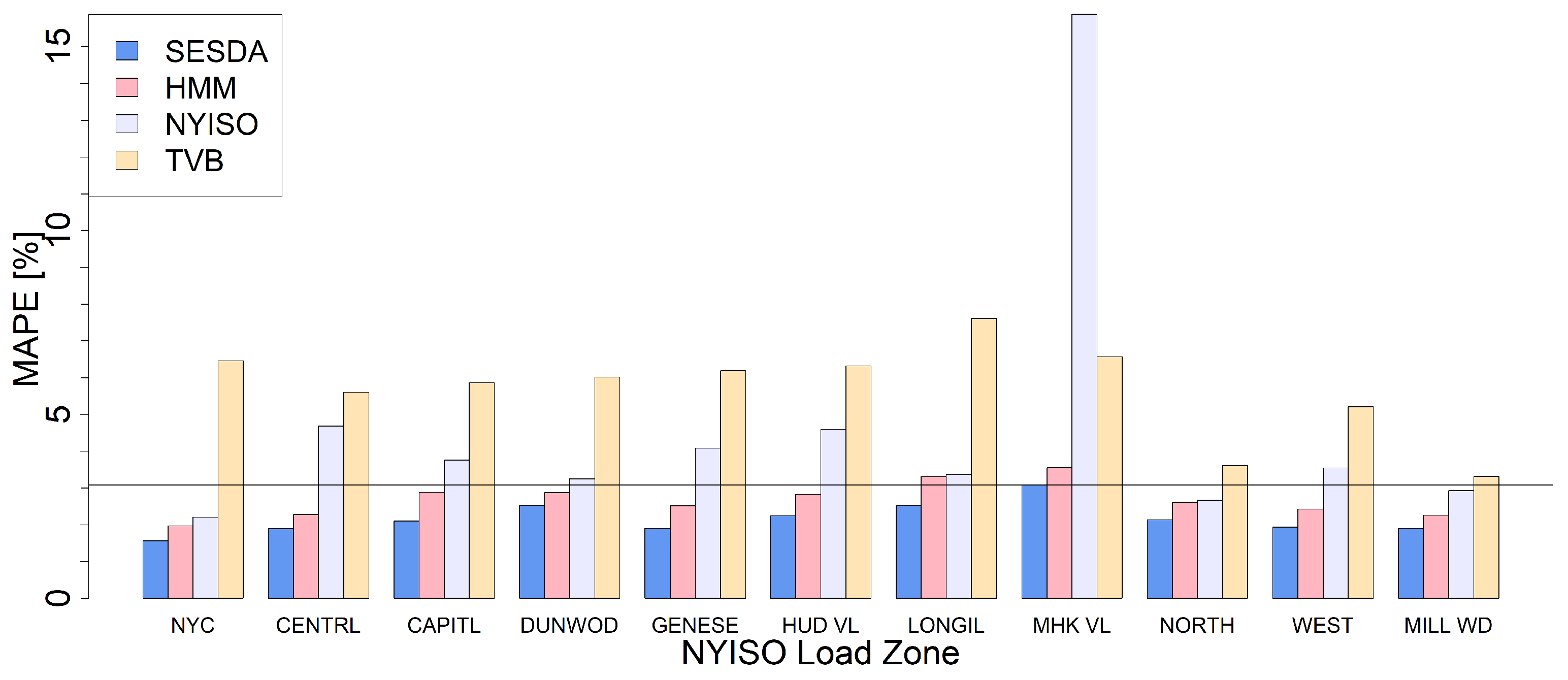
Figure 8 compiles the forecast error for 2017 delivered by all considered methods for each NYISO load zone. The attended sequential encoder-stacked decoder (SESDA) achieves the best results for all zones. It is, however, closely followed by the Hidden Markov Model with no training. The NYISO approach which combines regression with the usage of neural networks outperforms Tao’s Vanilla Benchmark but seems to have some problems with the low load zone MHK VL. For this zone, all approaches deliver relatively high error which may be related to quite a wide area (15,230 square kilometers) and a small population of that zone.
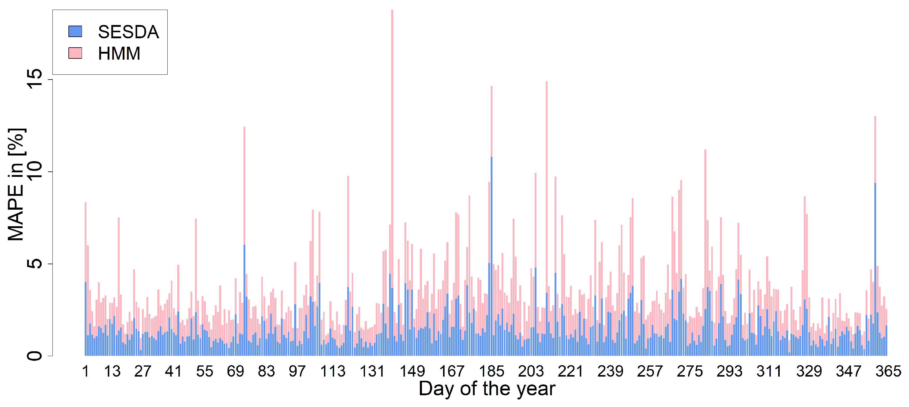
Figure 9 compares the daily MAPE for 2017 in New York City calculated using the two best approaches: SESDA and HMM. The SESDA approach returns a smaller error. The largest MAPE value for HMM is around 20% around 139th day of the year. Generally, the highest HMM errors are concentrated between May and September. The highest attended sequential encoder-stacked decoder error is around 10%. It occurs on holidays, on 4 July 2017 and 25 December 2017. Moreover, the higher forecast error on average, the HMM approach delivers also more and higher error peaks on problematic days.
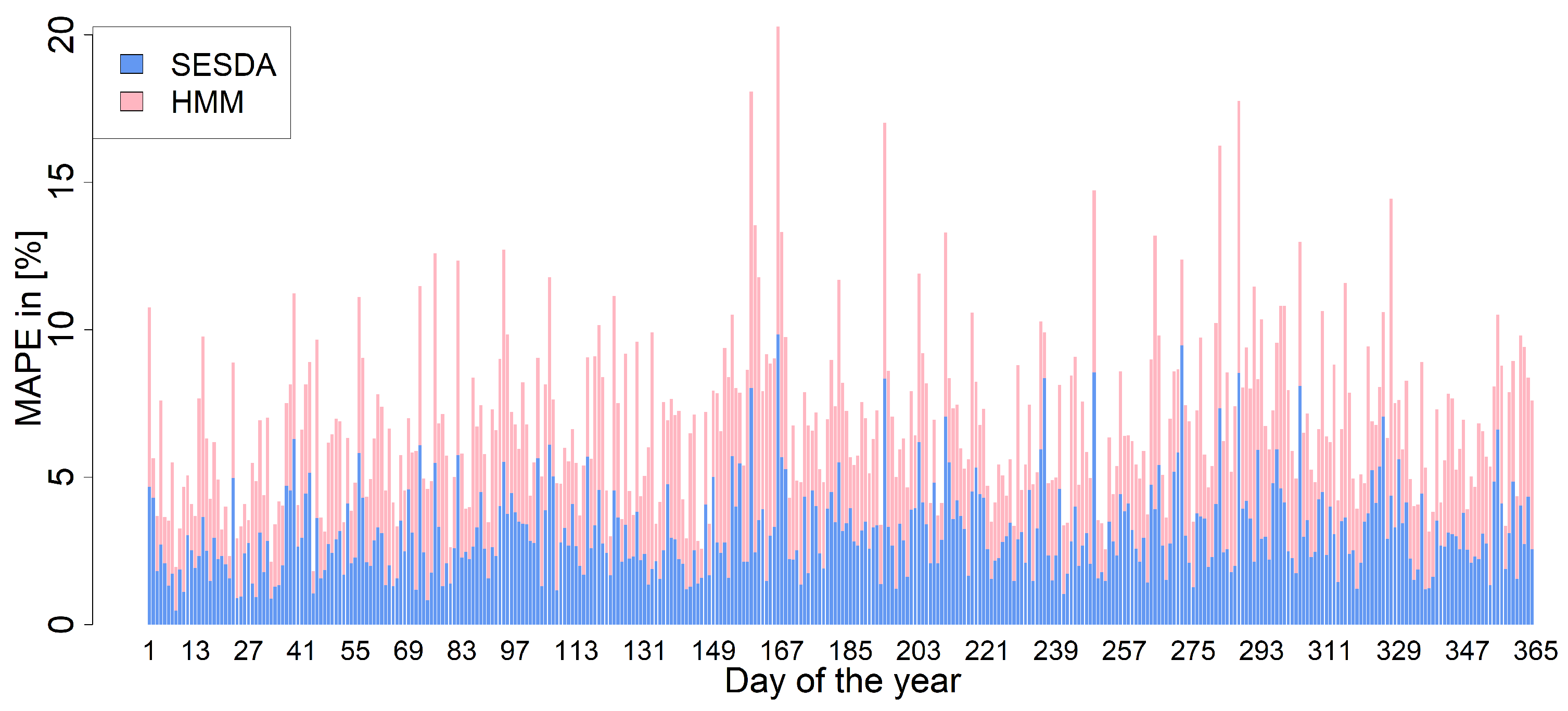
Figure 10 compiles the results of SESDA and HMM evaluated for each day of 2017 in the load zone Mohawk Valley (MHK VL). The highest error delivered by the SESDA approach is around 10% and occurs on around the 165 and the 275th day of the year. The HMM produces the highest error of around 20% also around 165. day of the year. On several days of the year, the MAPE returned by the HMM exceeds the 10% limit. The SESDA approach delivers therefore more stable results with significantly smaller error peaks.
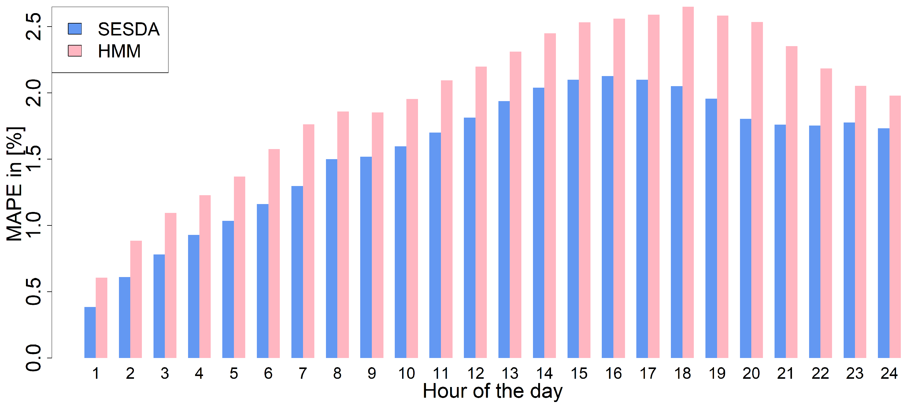
Figure 11 shows forecast errors in New York City according to the hour of the day. For each hour the SESDA model outperforms the HMM reducing significantly the forecast errors.
Table 2 shows the evaluation of different ANN approaches on the NYC data set. Among all approaches, the best results are achieved with the sequential encoder and stacked decoder architecture. Sequential encoder-decoder with attention performs only a little better than the sequential encoder-decoder without attention because it shares the attention layer for all time instances. Sequential encoder-decoder without attention performs only slightly better than the LSTM network. The reason is too strong context vector compression in a 24 instances encoder. The LSTM network used for the evaluation consists of 24 inputs. The 24th input is the predicted one. The model is trained for each prediction hour separately. The Nonlinear Autoregressive Network with Exogenous inputs (NARX) [19] shows the worst results. It has been implemented using 24 dense networks for every prediction hour each.
The encoder-decoder method has been evaluated on a personal computer with Intel Core i5-6300U [email protected] GHz and 32 GB RAM. For the implementation, the Python programming language along with the Tensorflow [34] and Keras libraries [35] has been used. An average execution time for 24 h ahead forecast took around 10 s (including loading test data, picking the most similar data, loading the weights into the model, training, and inference). The required amount of time is around 5 times larger in comparison to the HMM approach [29].

4. Conclusions

The presented approach uses a sequential encoder-stacked decoder architecture in combination with attention (SESDA) to predict load power 24 h ahead. The training data are collected using the smallest Euclidean distance between the daily features of the forecasted day and the days in the past. For each forecast day, a fast online training is executed using the filtered most similar past data. The features included in the encoder-decoder model range from hourly weather parameters, calendar data to the load demand from the previous hour.
The algorithm achieves the best results in comparison with the benchmark methods which include Linear Regression, a combination of Linear Regression and the usage of Neural Networks, and the Hidden Markov Model approach. Although the difference between the MAPE values of HMM and the encoder-decoder model is not as large as the difference between HMM and Linear Regression, the HMM seems less stable than the proposed architecture. However, the error reduction comes at a cost of the increased forecast execution time.
One of the limitations of the algorithm is the requirement of the availability of pairs of consecutive daily data for the training due to the network architecture (encoder-decoder model). For data with many gaps related to whole days, the algorithm may perform less successfully. Additionally, the algorithm requires on average 96 historical time series including the previous days for the training. If the requirement is not fulfilled, the prediction error will increase depending on the number of data provided. However, today’s utilities have mostly access to the required amount of data.
The approach can be extended to support longer time horizons. However, in this case some modifications of the architecture must be applied. First of all, the length of the encoded sequence must be adjusted to the length of the forecast sequence. Additionally, the self-attention mechanism inside of the decoder has to be used to consider the impact of the preceding predicted values on the following ones due to the longer time horizon.
In future work, the authors will draw their attention to the application of reinforcement learning to the area of short-term load forecasting.

Author Contributions

Conceptualization, S.H.; methodology, S.H. and M.G.; software, S.H.; validation, S.H. and M.G.; formal analysis, S.H. and M.G.; writing-original draft preparation, S.H.; writing-review and editing, S.H. and M.G. All authors have read and agreed to the published version of the manuscript.

Funding

This research received no external funding.

Institutional Review Board Statement

This article does not contain any studies with humans or animals.

Informed Consent Statement

This article does not contain any studies with humans or animals.

Data Availability Statement

https://www.nyiso.com/load-data (accessed on 26 May 2021).

Conflicts of Interest

The authors declare no conflict of interest.

Sample Availability

A prototype of the attended encoder-decoder is provided at https://github.com/sylwia-lab/LoadForecastEncoderDecoder/ (accessed on 26 May 2021).

References

  1. Srivastava, A.K.; Pandey, A.S. Short-term load forecasting methods: A review. In Proceedings of the 2016 International Conference on Emerging Trends in Electrical Electronics & Sustainable Energy Systems (ICETEESES), Sultanpur, India, 11–12 March 2016; pp. 130–138. [Google Scholar]
  2. Papalexopoulos, A.D.; Hesterberg, T.C. A regression-based approach to short-term system load forecasting. IEEE Trans. Power Syst. 1990, 5, 1535–1547. [Google Scholar] [CrossRef]
  3. Hong, T. Short Term Electric Load Forecasting; North Carolina State University: Raleigh, NC, USA, 2010. [Google Scholar]
  4. Trull, O.; García-Díaz, J.C.; Troncoso, A. Application of Discrete-Interval Moving Seasonalities to Spanish Electricity Demand Forecasting during Easter. Energies 2019, 12, 1083. [Google Scholar] [CrossRef] [Green Version]
  5. Shilpa, G.; Sheshadri, G. Short-Term Load Forecasting Using ARIMA Model For Karnataka State Electrical Load. Int. J. Eng. Res. Dev. 2017, 13, 75–79. [Google Scholar]
  6. Mpawenimana, I.; Pegatoquet, A.; Roy, V.; Rodriguez, L.; Belleudy, C. A comparative study of LSTM and ARIMA for energy load prediction with enhanced data preprocessing. In Proceedings of the 2020 IEEE Sensors Applications Symposium (SAS), Sundsvall, Sweden, 2–4 August 2020; pp. 1–6. [Google Scholar]
  7. Singhal, R.; Choudhary, N.K.; Singh, N. Short-Term Load Forecasting Using Hybrid ARIMA and Artificial Neural Network Model. In Advances in VLSI, Communication, and Signal Processing; Lecture Notes in Electrical Engineering; Dutta, D., Kar, H., Kumar, C., Bhadauria, V., Eds.; Springer: Berlin/Heidelberg, Germany, 2020; pp. 935–947. [Google Scholar]
  8. Ganguly, P.; Kalam, A.; Zayegh, A. SHORT TERM LOAD FORECASTING USING FUZZY LOGIC. In Proceedings of the 2016 International Symposium on Electrical Engineering (ISEE), Hong Kong, China, 14 December 2017; pp. 1–7. [Google Scholar]
  9. Al-Kandari, A.M.; Soliman, S.A.; El-Hawary, M. Fuzzy short-term electric load forecasting. Int. J. Electr. Power Energy Syst. 2004, 26, 111–122. [Google Scholar] [CrossRef]
  10. Ding, N.; Benoit, C.; Foggia, G.; Besanger, Y.; Wurtz, F. Neural Network-Based Model Design for Short-Term Load Forecast in Distribution Systems. IEEE Trans. Power Syst. 2016, 31, 72–81. [Google Scholar] [CrossRef]
  11. Tian, C.; Ma, J.; Zhang, C.; Zhan, P. A Deep Neural Network Model for Short-Term Load Forecast Based on Long Short-Term Memory Network and Convolutional Neural Network. Energies 2018, 11, 3493. [Google Scholar] [CrossRef] [Green Version]
  12. Peng, T.M.; Hubele, N.F.; Karady, G. Advancement Short-Term in the Application of Neural Networks for Load Forecasting. Trans. Power Syst. 1992, 7, 250–257. [Google Scholar] [CrossRef]
  13. Kiartzis, S.; Bakirtzis, A.; Petridis, V. Short-term load forecasting using neural networks. Electr. Power Syst. Res. 1995, 33, 1–6. [Google Scholar] [CrossRef]
  14. Wu, W.; Liaob, W.; Miaoa, J.; Du, G. Using Gated Recurrent Unit Network to Forecast Short-Term Load Considering Impact of Electricity Price. In Proceedings of the 10th International Conference on Applied Energy (ICAE2018), Hong Kong, China, 22–25 August 2018; pp. 3369–3374. [Google Scholar]
  15. Zheng, J.; Xu, C.; Zhang, Z.; Li, X. Electric Load Forecasting in Smart Grid Using Long-Short-Term-Memory based Recurrent Neural Network. In Proceedings of the 2017 51st Annual Conference on Information Sciences and Systems (CISS), Baltimore, MD, USA, 22–24 March 2017; pp. 1–6. [Google Scholar]
  16. Kuo, P.H.; Huang, C.J. A High Precision Artificial Neural Networks Model for Short-Term Energy Load Forecasting. Energies 2018, 11, 213. [Google Scholar] [CrossRef] [Green Version]
  17. Bouktif, S.; Fiaz, A.; Ouni, A.; Serhani, M.A. Optimal Deep Learning LSTM Model for Electric Load Forecasting using Feature Selection and Genetic Algorithm: Comparison with Machine Learning Approaches. Energies 2018, 11, 1636. [Google Scholar] [CrossRef] [Green Version]
  18. Bouktif, S.; Fiaz, A.; Ouni, A.; Serhani, M.A. Multi-Sequence LSTM-RNN Deep Learning and Metaheuristics for Electric Load Forecasting. Energies 2020, 13, 391. [Google Scholar] [CrossRef] [Green Version]
  19. Bianchi, F.M.; Maiorino, E.; Kampffmeyer, M.C.; Rizzi, A.; Jenssen, R. Recurrent Neural Networks for Short-Term Load Forecasting. An Overview and Comparative Analysis; Springer: Cham, Switzerland, 2017. [Google Scholar]
  20. Lu, K.; Meng, X.R.; Sun, W.X.; Zhang, R.G.; Han, Y.K.; Gao, S.; Su, D. GRU-based Encoder-Decoder for Short-term CHP Heat Load Forecast. IOP Conf. Ser. Mater. Sci. Eng. 2018, 392, 1–7. [Google Scholar] [CrossRef]
  21. Bahdanau, D.; Cho, K.H.; Bengio, Y. Neural Machine Translation by Jointly Learning to Align and Translate. arXiv 2015, arXiv:1409.0473. [Google Scholar]
  22. Sehovac, L.; Grolinger, K. Deep Learning for Load Forecasting: Sequence to Sequence Recurrent Neural Networks with Attention. IEEE Access 2020, 8, 36411–36426. [Google Scholar] [CrossRef]
  23. Meng, Z.; Xu, X. A Hybrid Short-Term Load Forecasting Framework with an Attention-Based Encoder–Decoder Network Based on Seasonal and Trend Adjustment. Energies 2019, 12, 4612. [Google Scholar] [CrossRef] [Green Version]
  24. Jin, X.B.; Zheng, W.Z.; Kong, J.L.; Wang, X.Y.; Bai, Y.T.; Su, T.L.; Lin, S. Deep-Learning Forecasting Method for Electric Power Load via Attention-Based Encoder-Decoder with Bayesian Optimization. Energies 2021, 14, 1596. [Google Scholar] [CrossRef]
  25. Pan, S.J.; Yang, Q. A Survey on Transfer Learning. IEEE Trans. Knowl. Data Eng. 2010, 22, 1345–1359. [Google Scholar] [CrossRef]
  26. Hooshmand, A.; Sharma, R. Energy Predictive Models with Limited Data using Transfer Learning. arXiv 2019, arXiv:1906.02646. [Google Scholar]
  27. Ribeiro, M.; Grolinger, K.; ElYamany, H.; Higashino, W.A.; Capretz, M. Transfer learning with seasonal and trend adjustment for cross-building energy forecasting. Energy Build. 2018, 165, 352–363. [Google Scholar] [CrossRef]
  28. NYISO. Load Data. 2019. Available online: https://www.nyiso.com/load-data (accessed on 26 May 2021).
  29. Henselmeyer, S.; Grzegorzek, M. Short-term load forecasting with discrete state Hidden Markov Models. J. Intell. Fuzzy Syst. 2020, 38, 2273–2284. [Google Scholar] [CrossRef]
  30. Mandal, P.; Senjyu, T.; Urasaki, N.; Funabashi, T. A neural network based several-hour-ahead electric load forecasting using similar days approach. Electr. Power Energy Syst. 2006, 28, 367–373. [Google Scholar] [CrossRef]
  31. Yurafsky, D.; Martin, J. Speech and Language Processing; Prentice Hall: Upper Saddle River, NJ, USA, 2008. [Google Scholar]
  32. Operations, N.E.M. Day Ahead Scheduling Manual. 2017. Available online: https://www.nyiso.com/documents/20142/2923301/dayahd_schd_mnl.pdf/0024bc71-4dd9-fa80-a816-f9f3e26ea53a (accessed on 26 May 2021).
  33. Liu, B. Short Term Load Forecasting with Recency Effect: Models and Applications; ProQuest, UMI Dissertation Publishing: Ann Arbor, MI, USA, 2016. [Google Scholar]
  34. Abadi, M.; Agarwal, A.; Barham, P.; Brevdo, E.; Chen, Z.; Citro, C.; Corrado, G.S.; Davis, A.; Dean, J.; Devin, M.; et al. TensorFlow: Large-Scale Machine Learning on Heterogeneous Systems. arXiv 2015, arXiv:1603.04467. [Google Scholar]
  35. Chollet, F. Keras. 2015. Available online: https://keras.io (accessed on 26 May 2021).
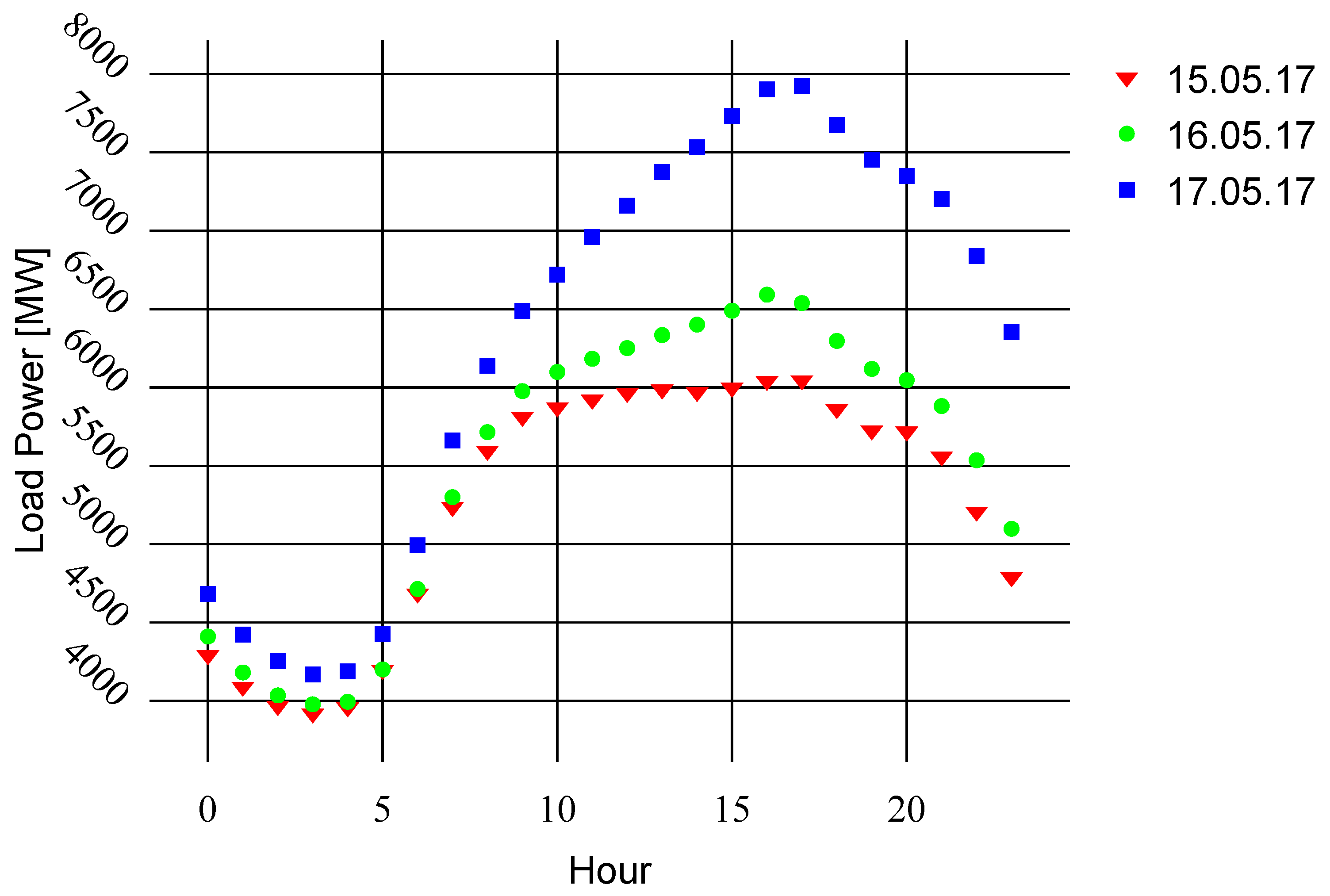
Figure 1. Load curves on subsequent days in May 2017 for the New York City data.
Applsci 11 04927 g001
Figure 2. Temperature curves on subsequent days in May 2017 for the New York City data.
Applsci 11 04927 g002
Figure 3. Correlation between temperature and load on subsequent days in May 2017 for the New York City data.
Applsci 11 04927 g003
Figure 4. A Long Short-Term Memory cell.
Applsci 11 04927 g004
Figure 5. An example of the encoder-decoder architecture with Long Short-Term Memory cells.
Applsci 11 04927 g005
Figure 6. Artifitial neural network architecture for load forecasting.
Applsci 11 04927 g006
Figure 7. Overview of the applied algorithm for training and inference.
Applsci 11 04927 g007
Figure 8. Evaluation of the 24 h ahead forecast error in 2017.
Applsci 11 04927 g008
Figure 9. Daily MAPE of a 24 h ahead forecast in NYC for 2017.
Applsci 11 04927 g009
Figure 10. Daily MAPE of a 24 h ahead forecast in MHK VL for 2017.
Applsci 11 04927 g010
Figure 11. Hourly MAPE of 24 h ahead forecast in NYC for 2017.
Applsci 11 04927 g011
Table 1. NYISO load zones.
Zone NameZone IDAverage Load [MW]
CapitalCAPITL1450
CentralCENTRL1900
DunwoodieDUNWOOD780
GeneseGENESE1200
Hudson ValleyHUD VL1200
Long IslandLONGIL2500
MillwoodMILL VD770
Mohawk ValleyMHK VL980
New York CityNYC6000
NorthNORTH590
WestWEST1800
Table 2. Results of different ANN approaches for NYC zone.
Method NameMAPE
Sequential Encoder Stacked Decoder with Attention1.52
Sequential Encoder-Decoder with Attention1.66
Sequential Encoder-Decoder1.72
LSTM1.75
NARX2.16
Publisher’s Note: MDPI stays neutral with regard to jurisdictional claims in published maps and institutional affiliations.