Article

Short Term Electric Load Forecasting Based on Data Transformation and Statistical Machine Learning

by
Nikos Andriopoulos
1,2,
Aristeidis Magklaras
1,
Alexios Birbas
1,*,
Alex Papalexopoulos
3,
Christos Valouxis
1,
Sophia Daskalaki
1,
Michael Birbas
1,
Efthymios Housos
1 and
George P. Papaioannou
2
1
Department of Electrical and Computer Engineering, University of Patras, 265 00 Patras, Greece
2
Research, Technology & Development Department, Independent Power Transmission Operator (IPTO) S.A., 89 Dyrrachiou & Kifisou Str. Gr, 104 43 Athens, Greece
3
Ecco International Inc., San Francisco, CA 94104, USA
*
Author to whom correspondence should be addressed.
Appl. Sci. 2021, 11(1), 158; https://doi.org/10.3390/app11010158
Submission received: 4 December 2020 / Revised: 22 December 2020 / Accepted: 23 December 2020 / Published: 26 December 2020
(This article belongs to the Special Issue Advanced Methods of Power Load Forecasting)

Abstract

:
The continuous penetration of renewable energy resources (RES) into the energy mix and the transition of the traditional electric grid towards a more intelligent, flexible and interactive system, has brought electrical load forecasting to the foreground of smart grid planning and operation. Predicting the electric load is a challenging task due to its high volatility and uncertainty, either when it refers to the distribution system or to a single household. In this paper, a novel methodology is introduced which leverages the advantages of the state-of-the-art deep learning algorithms and specifically the Convolution Neural Nets (CNN). The main feature of the proposed methodology is the exploitation of the statistical properties of each time series dataset, so as to optimize the hyper-parameters of the neural network and in addition transform the given dataset into a form that allows maximum exploitation of the CNN algorithm’s advantages. The proposed algorithm is compared with the LSTM (Long Short Term Memory) technique which is the state of the art solution for electric load forecasting. The evaluation of the algorithms was conducted by employing three open-source, publicly available datasets. The experimental results show strong evidence of the effectiveness of the proposed methodology.

1. Introduction

Load forecasting has always been a challenging task that triggers the interest of both academia and the industrial sector. Since the 1960s, auto-regressive (AR) models have been widely used for designing and implementing predictive load forecasting models. These were based on the assumption that the system/substation load at any given time can be satisfactorily described as a linear combination of past load values and other values of a set of exogenous variables. Therefore, they were either plain AR models or AR models with exogenous variables (ARX) and/ or AR models with moving average components (ARMA and ARMAX). Such models and variants thereof were used extensively for electric load forecasting [1,2].
The linearity assumption was relaxed with the development of machine learning-based models such as neural networks [3,4] and kernel-based methods (e.g., support vector machines [5]). Neural networks are nowadays the most widely used machine learning tool for nonlinear regression in electrical load forecasting. At the same time, support vector regression is gaining popularity in this area [6].
In this paper we focus on the state-of-the-art Artificial Neural Network (ANN) deep learning algorithms, namely the Convolution Neural Nets (CNNs) in order to perform load prediction. Currently the most successful and popular algorithm in literature for addressing this issue is the use of Long Short Term Memory (LSTM) [7] method, which belongs to the Recurrent Neural Network (RNN) architectural type and exploits the short and long term relationships that exist in a data series in order to build a predictive model. LSTM algorithms are considered to be the most suitable choice for electric load forecasting compared to other neural network architectures. CNNs, on the other hand, are considered to be the preferred choice for image processing related tasks, like image recognition, due to their ability to take advantage of the inherent stationarity usually observed in the pixel data, thus resulting in more accurate models. Nevertheless, it will be shown that CNN-based models can also provide efficient solutions for the electric load forecasting problem and under certain conditions, such as applying proper data preprocessing and analysis, they could even outperform the LSTM-based models.
Despite the black box nature of ANN solutions, there is considerable freedom for differentiating model selection choices and parameter tuning, such as the number of epochs, batch size or hidden dimensions and filters (i.e., the number of output filters in the convolution) for the CNN-based models. The proposed approach offers a comprehensive methodology for model selection and parameter tuning resulting in significantly lower forecasting errors compared to the LSTM model. Furthermore, the data transformation which was performed after extensive statistical analysis allows optimal input selection for our models. The most common input in such cases is the previous state (t-1) of the forecasted variable. This leads to higher accuracy for uni-step forecasting applications, but at the same time it lowers the performance of the multi-step ones by introducing several defects. In our case, the input value is derived directly from the results of statistical analysis. It is important to mention that this paper does not focus on the CNN algorithm itself, but rather on the proper statistical analysis (pre-processing) which facilitates the data transformation based on data features (i.e., stationarity) and achieve best possible performance of the algorithm. The methodology and the different techniques employed will be thoroughly described in Section 2.
According to the time horizon used for prediction, load forecasting can be classified into very short-term load forecasting (VSTLF), short-term load forecasting (STLF), medium-term load forecasting (MTLF), and long-term load forecasting (LTLF). The forecasting horizon varies from 5 min, to one day, to two weeks or to three or more years; depending on the planning or operational function it supports [8].
Across literature a wide range of methodologies and models have been proposed to improve the accuracy of load forecasting, yet most of them are based upon aggregated power consumption data at the system (top) level with little to no information regarding power consumption profiles at the customer class level. This approach was acceptable till now, since the operational focus until recently had been on the bulk transmission system and the wholesale energy markets. Since the interest now is shifted towards the distribution system and the efficient integration of Distributed Energy Resources (DERs) connected close to the edge of the grid, this approach is not sufficient anymore. Hence, distribution substation load forecasting becomes a necessity for the Distribution System Operators (DSOs). Forecasting on distribution feeder has not been widely examined across literature. Low Voltage (LV) distribution feeders are more volatile compared to the high voltage (HV) ones, since they consist of low aggregations of consumers [9]. One approach is to adopt the forecasting techniques and models that are currently employed at higher voltage levels. The main forecasting research in these areas has been presented in [10,11], that apply both ARIMAX and ANN methods to a single LV transformer (consisting of 128 customers) for forecasting the total energy and peak demand. In their method they take into account historical weather data and they achieve MAPEs of 6–12%. In [12] a three-stage methodology, which consists of pre-processing, forecasting, and post-processing, was applied to forecast loads of three datasets ranging from distribution level to transmission level. A semi-parametric additive model was proposed in [13] to forecast the load of Australian National Electricity Market. The same technique was also applied to forecast more than 2200 substation loads of the French distribution network in [14]. Another load forecasting study on seven substations from the French network was performed in [15], where a conventional time series forecasting methodology was utilized. In [16], the authors proposed a neural network model to forecast the load of two French distribution substations, which outperformed a time series model. It is focused on developing a methodology for neural network design in order to obtain a model that has the best achievable predictive ability given the available data. Variable selection and model selection was applied to electrical load forecasts to ensure an optimal generalization capacity of the neural network model.
Exponential smoothing model and its variations, such as double and triple seasonal exponential smoothing ones, have also showcased good results [17] but are less popular in real-life applications due to their inability to accommodate exogenous variables. Another popular approach, denoted as hybrid, is to combine different models as in [1] where Principal Component Analysis (PCA) and Multiple Linear Regression (MLR) are combined for daily load predictions.
For LV networks accurate load forecasting can be employed to support a number of operations, including demand side response [18], storage control [19,20] and energy management systems [21,22]. Load forecasting for low scale consumers, such as residential loads, is valuable for home energy management systems (HEMS) [23] while house level load forecasting can play a significant role in the future Local Energy Markets (LEM) which will facilitate the energy transactions among participants [24]. Load forecasting has been implemented for either the HV or system level and typically consists of the aggregated demand of hundreds of thousands or millions of consumers. Such demand is much less volatile than the LV demand, and hence, is easier to predict. Load forecasting at this level is very mature research-wise and there is a great volume of literature describing and testing a number of methods and algorithms, including ANNs, Support Vector Machine (SVM), ARIMA, exponential smoothing, fuzzy systems, and linear regression. Recent methods upon load forecasting can be found in [25].
However, the loads of a house, a factory, and a feeder are more volatile than HV level loads. Therefore, developing a highly accurate forecast at lower consumption levels is nontrivial. Although the majority of the load forecasting literature has been dedicated to forecasting at the top (high voltage) level, the information from medium/low voltage levels offers a promising field of research. The highly volatile nature of house load time series makes it particularly difficult to achieve very accurate predictions. In [26] the authors showed that the ‘‘double peak’’ error for spiky data sets means that it is difficult to measure the accuracy of household-level point forecasts objectively introducing traditional pointwise errors. Similar methods have been applied at the household level as at the HV level, including ANNs [27,28] ARIMAs, wavelets [29], Kalman filters [30] and Holt-Winters exponential smoothing [31]. The prediction errors of these methods are much higher compared to those reported at the HV level, with MAPEs ranging from 7% up to 85% in some cases.
Regardless the voltage level and the load scale, load forecasting problems share certain common factors that may affect the prediction accuracy of energy consumption. These are the energy markets, the variables affected by the weather and the hierarchical topology of the grid. In competitive energy retail markets, the electricity consumption is largely driven by the number of customers. Since the number of customers is uncertain, the load profile is consequently characterized by high stochasticity. In [32] the authors propose a two-stage long-term retail load forecasting method to take customer reduction into consideration. The first stage forecasts each customer’s load using multiple linear regression with a variable selection method. The second stage forecasts customer attrition using survival analysis. Then, the final forecast results from the product of the two forecasts. Another issue regarding the energy market is the demand response programs which pose another challenge in load forecasting, since some consumers are willing to alter their consumption patterns according to price signals, while others are not. In [33] the authors detect the price-driven customers by applying a non-parametric test so that they can be forecasted separately. Across literature, many papers have shown strong correlations between weather effects and demand. A weather variable investigated in literature is humidity [34], where the authors discovered that the temperature-humidity index (THI) may not be optimal for load forecasting models. Instead, more accurate load forecasts than the THI-based models were performed when the authors separated relative humidity, temperature and their higher order terms and interactions in the model, with the corresponding parameters being estimated by the training data. In [35] the load of a root node of any sub-tree was forecasted first. The child nodes were then treated separately based on their similarities. The forecast of a “regular” node was proportional to that of the parent node, while the “irregular” nodes were forecasted individually using neural networks. In [36] the authors exploit the hierarchical structure of electricity grid for load forecasting. Two case studies were investigated, one based on New York City and its substations, and the other one based on Pennsylvania-New Jersey-Maryland (PJM) and its substations. The authors demonstrated the effectiveness of aggregation in improving the higher level load forecast accuracy.
The availability of data from Advanced Metering Infrastructure (AMI) systems enables the use of novel approaches to the way load forecasting is performed, ranging from the distribution level to even the residential scale. In existing literature, researchers have focused on: (1) longitudinal and (2) cross-sectional grouping methods trying to handle efficiently load data. Longitudinal grouping refers to identifying time periods with similar load patterns, which are derived from statistical analysis based on historical data. On the other hand, cross-sectional grouping refers to the aggregation of customers with similar consumption characteristics. In [37] the authors examined six methods which are usually employed in large-scale energy systems to predict a load similar to that of a single transformer. The models that were investigated were ANNs, AR, ARMA, autoregressive integrated moving average, fuzzy logic, and wavelet NNs for day-ahead and week-ahead electric load forecasting in two scenarios with different number of houses. In [38] a clustering based on AMI data is performed among customers to identify groups with similar load patterns prior to performing load forecasting, in favor of forecasting accuracy. In [39], the authors implemented a neural network (NN)-based method for the construction of prediction intervals (PIs) to quantify potential uncertainties associated with forecasts. A newly introduced method, called lower upper bound estimation (LUBE), is applied and extended to develop PIs using NN models. In [40] a new hybrid model is proposed. This model is a combination of the manifold learning Principal Components (PC) technique and the traditional multiple regression (PC-regression), for short and medium-term forecasting of daily, aggregated, day-ahead, electricity system-wide load in the Greek Electricity Market for the period 2004–2014. PC-regression is compared with a number of classical statistical approaches as well as with the more sophisticated artificial intelligence models, ANN and SVM. The authors have concluded that the forecasts of the developed hybrid model outperforms the ones generated by the other models, with the SARIMAX model being the next best performing approach, giving comparable result.
The advantages that smart meters bring to load forecasting are two-fold. Firstly, smart meters offer the opportunity to distribution companies and electricity retailers to better understand and forecast the load of small scale consumers. Secondly, the high granularity and volume of load data provided by smart meters may improve the forecast accuracy of the models on the grounds that the training dataset will be more representative and will capture the highly volatile demand patterns that describe the load behavior of households or buildings. Therefore, the traditional techniques and methods developed for load forecasting at an aggregate level may not be well suited. Many different approaches are currently examined, all attempting to leverage the large volume of data derived from the numerous operating smart meters so as to improve the forecasting accuracy. In [41] seven existing techniques, including linear regression, ANN, SVM and their variants were examined. The case study was conducted on two datasets, one comprising of two commercial buildings and the other of three residential homes. The study demonstrated that these techniques could produce forecasts with high accuracy for the two commercial loads, but did not perform well for the residential ones. In [29] a self-recurrent wavelet neural network (SRWNN) was proposed to forecast the load for a building within a microgrid. The proposed SRWNN was shown to be more accurate than its ancestor wavelet neural network (WNN) for both building level and higher level load cases. Deep learning techniques for the household and building-level load forecasting are also employed across literature. In [42] a pooling-based deep RNN was proposed to learn spatial information shared between interconnected customers and to address the over-fitting problems. The proposed method outperformed ARIMA, SVR, and classical deep RNN on the Irish CER residential dataset. In [43] a spatio-temporal forecasting approach was proposed to leverage the sparsity which is a valuable element in small scale load forecasting. The proposed method combined ideas from compressive sensing and data decomposition to exploit the low-dimensional structures governing the interactions among the nearby houses. The dataset upon which the method was examined was the Pecan Street dataset.
Additional categorization among the different load forecasting methods in the literature can be summarized as follows: (1) Physics principles-based models and (2) Statistical/Machine learning-based models. In [44] ANNs were used to perform load forecasting in buildings. Finally, in [45] a short-term residential load forecasting based on resident behavior learning was examined. RNNs, such as LSTM, seem as a reasonable selection for time series applications since they are developed explicitly to handle sequential data. In [46] a custom Deep Learning model that combines multiple layers of CNNs for feature extraction is presented, where both LSTM layers (prediction) and parallel dense layers (transforming exogenous variables) are proposed. Finally in [47] a novel method to forecast the electricity loads of single residential households is proposed based on CNNs (combined with a data-augmentation technique), which can artificially enlarge the training data in order to face the lack of sufficient data.
This work focuses on a statistical learning-based approach by examining and leveraging the special statistical features of each given dataset [48] and thereafter transforming the dataset into a form according to the statistical analysis performed for that purpose. Our framework is based on the employment of a CNN architecture. CNNs are among the most popular techniques for deep learning, mainly for image processing tasks [49], where they leverage the spatial locality of pixels. There have been recently presented remarkable efforts of using CNN models for electrical load forecasting [50]. CNNs choice is based on the fact that in load time series, two neighboring points do not exhibit significant deviation. Therefore, load time series are characterized by temporal locality which can be exploited by CNNs. In this paper, we demonstrate that LSTMs for load forecasting under certain conditions can be outperformed; this finding is supported by experimental evidence. To prove our point, we furthermore compare our CNN model with three other machine learning techniques, namely LSTM, ANN and Multilayer Perceptron (MLP). The main contributions of the paper can be summarized in the following:
  • We introduce a method for properly tuning the model’s parameters by taking into account the time series statistical properties and especially its auto correlation.
  • We offer a valid alternative to the load forecasting problem in the case of low scale energy deployments where it is derived that our CNN based approach is more efficient than other methods.
  • We identify the conditions under which the CNN outperforms the other widely used forecasting solutions such as high temporal relationship between time series observations, lack of historical data and low scale load consumption.
  • We offer a solution to times series forecasting in cases where there is shortage of training data, since in our experiments the historical data available for training were limited.
The rest of the paper is organized as follows: In Section 2 the proposed methodology is analyzed in detail, in Section 3 the results of our investigation is given and in Section 4 we present the discussion and the conclusions of our work and suggest possible future research extensions.

2. Proposed Methodology

2.1. Convolutional Neural Networks (CNN)

CNN is a class of deep neural networks, most commonly applied to analyzing visual imagery. They are also known as shift invariant or space invariant artificial neural networks (SIANN), based on their shared-weights architecture and translation invariance characteristics [51,52]. CNNs are regularized versions of multi-layer perceptron but they take a different approach towards regularization, since they take advantage of the hierarchical form in data and assemble more complex patterns using smaller and simpler patterns. Therefore, on the scale of connectivity and complexity, CNNs are functioning on the lower extreme. CNNs use relatively little pre-processing compared to other image classification algorithms. This means that the network trains the filters that in traditional algorithms were hand-engineered. This independence from prior knowledge and human effort in feature design is a major advantage.
As presented in Figure 1, a CNN consists of an input and an output layer, as well as multiple hidden layers. These layers perform operations that alter data with the intent of extracting features specific to the data. Three of the most common layers are: convolution, activation or ReLU, and pooling. The hidden layers of a CNN typically consist of a series of convolutional layers that convolve through multiplication or other dot product each of which activates certain image features.
The input layer reads an input image into the CNN. It consists of various low-level image-processing functions to pre-process the input image as an appropriate data type for the minimal CNN. Practically, the size of the input image is preferably on the order of power of 2 so that to ensure computation efficiency for a CNN. However, input images with uneven row-column dimensions can also be used. The convolution layer extracts pixel-wise visual features from an input image [54,55,56]. The trainable convolution kernels in this layer adjust their (kernel) weights automatically through back-propagation to learn the input image features [56,57]. Image features learned by the convolution layer allow the successive algorithmic layers to process the extracted image features for other computational operations. The convolution layer is the dot product of the input image I and the kernel used, K. The result is a convolved feature map, f c which is derived by the Equation (1).
f c = c o n v ( i , j ) = ( I K ) ( i , j ) = m n I ( m , n ) K ( i m , j n )
Here ⊗ denotes a two-dimensional discrete convolution operator. Equation (1) shows that the convolution kernel K spatially slides over the input image I to compute the element-wise multiplication and sum to produce an output, a convolved feature map f c . Convolution provides weights sharing, sparse interaction (and local connectivity), and equivariant representation for unsupervised feature learning. More in depth technical details on these convolution properties can be found in [54,55,57,58,59,60]. The activation function is commonly a Rectified Linear Unit ( R e L U ) layer. R e L U allows for faster and more effective training by mapping negative values to zero and maintaining positive values. This is sometimes referred to as activation, because only the activated features are carried forward to the next layer. The objective of the R e L U layers is to introduce a point-wise nonlinearity to a CNN, which allows it to learn through a nonlinear input function. R e L U has also proven to be an effective solution to resolve vanishing gradient problems when training a CNN using the backpropagation algorithm [55,56]. The mathematical structure of the ReLU function is a piecewise nonlinear operator with a max output indicative function [54,58]. The output of a R e L U is a rectified feature map, f r that can be obtained by Equation (2).
f r = R e L U ( x i ) = m a x ( 0 , x i )
Equation (2) produces zero for negative inputs and linearly conveys the input for positive inputs. The activation layer is followed by pooling layers which simplify the output by performing nonlinear down-sampling, thus reducing the number of parameters that the network needs to learn, controlling the overfitting by progressively reducing the spatial size of the network and reducing the computational burden in the network. Those layers are referred to as hidden layers because their inputs and outputs are masked by the activation function and final convolution. The final convolution, in turn, often involves backpropagation in order to more accurately weight the end product.
Though the layers are colloquially referred to as convolutions, this is only by convention. Mathematically or technically, it is a sliding dot product or cross-correlation. This is significant for the indices in the matrix, in the sense that it affects how the weight is determined at a specific index point.
This special design of CNNs renders them capable to successfully capture the spatial and temporal dependencies in an image through the application of the relevant afore-described filters. The architecture shows a better fitting to the image dataset due to the reduction in the number of parameters involved and reusability of weights. In other words, the network can be trained to understand the sophistication of the image better. In this context, a CNN-based methodology is analyzed to evaluate its performance for forecasting applications with short period datasets with the motivation behind the CNN-based approach being its wide usage for image recognition applications. More specifically, the CNN models exploit the spatial locality of the pixel data in order to recognize an image. Similarly, in load time series, time locality, expressed by data stationarity and autocorrelation, forms the main motivation for utilizing CNN-based models in load forecasting applications. In our approach we transform the time series data into image-like data, taking advantage of the autocorrelation excibited by time series. Therefore, the first step is to perform statistical analysis and test the data for stationarity. If the data are not stationary then a second step of stationarity analysis is conducted by deploying a Unit Root Test, in order to capture more complex forms of stationarity, which is the case in most datasets.

2.2. Load Time Series Formulation and Statistical Analysis

The time-varying nature of both residential and community electrical load datasets is modeled by deploying smaller auto-regressive data models. An autoregressive model depicts that the output variable depends linearly on its own previous values and on a stochastic term, therefore the model is in the form of a stochastic difference equation. Specifically, an autoregressive model of order p is defined as in Equation (3):
X t = c + i = 1 p ϕ i + X t 1 + e t
Here ϕ i are the parameters of the model, c is a constant, and e t is the error, where E ( e t ) = 0 and V a r ( e t ) = σ 2 .
The stationarity of the load time series is explored by deploying the unit root test [61]. A linear stochastic process has a unit root, if 1 is a root of the process’ characteristic equation. Such a process is non-stationary but does not always have a trend. If the other roots of the characteristic equation lie inside the unit circle—that is, have a modulus (absolute value) less than one—then the first difference of the process will be stationary; otherwise, the process will need to be differentiated multiple times to become stationary. Due to this characteristic, unit root processes are also called difference stationary. Unit root processes may sometimes be confused with trend-stationary processes; while they share many properties, they are different in many aspects. It is possible for a time series to be non-stationary, yet to have no unit root and be trend-stationary. In both unit root and trend-stationary processes, their mean average may be increasing or decreasing over time; however, in the presence of a shock, trend-stationary processes are mean-reverting. The previous discrete-time stochastic process can be rewritten as an autoregressive process of order p:
X t = α 1 x t 1 + α 2 x t 2 + + α p x t p + e t
and
E ( X t | X t 1 , , X p ) = i = 1 p α i X t i
The time series is a serially uncorrelated, zero-mean stochastic process with constant variance σ 2 . If m = 1 is a root of the characteristic Equation (6) then the stochastic process has a unit root.
m p m p 1 α 1 m p 2 α 2 α p = 0
The stochastic process has a unit root or, alternatively, is 1st order integrated. If m = 1 with a root of multiplicity r, then the stochastic process is r t h integrated, denoted I ( r ) . There are various tests to check the existence of a unit root. In this paper we use the Augmented Dickey Fuller (ADF) [62] test which is widely used in statistics and econometrics. This analysis tests the null hypothesis that a unit root is present in a time series sample. If the unit root is not present then we cannot determine whether the time series is stationary. The ADF test is suitable for a large and more complicated set of time series models. The ADF index ( γ ) is a negative number; the more negative it is, the stronger the rejection of the hypothesis of non-stationarity for the observed level of significance is. As can be seen from Table 1, for all datasets the null hypothesis for non-stationarity has been rejected at the 0.01 significance level. Therefore it is quite likely that the electric load measured in all these cases displays the characteristic of trend or differential stationarity. The testing process of the ADF test is similar to the Dickey Fuller test but it is applied to the following model Equation (7).
Δ x t = α + β t + γ t 1 + δ Δ x t 1 + + δ p 1 Δ x t p + 1 + e t

2.3. Stationarity Analysis

The CNN structure is based on image as an input and for this reason the first step of our methodology is to transform the time series-sequential data into an appropriate, image-like form in order to be processed by the CNN. Image data can be more efficiently processed by CNNs because of their ability to handle the local stationarity of the respective pixels. Image data, namely pixels are characterized as highly stationary and this is the feature that our investigation will leverage. By detecting such behavior in our data we will accordingly transform our time series into “image” like structures. Electrical load data, as mentioned before, appear to have time stationarity.
In order to determine the stationarity of each dataset we calculate their sample means (Mean in Table 1) and standard deviations (STD in Table 1). In a stationary process the unconditional joint probability distribution (and consequently its mean and standard deviations) does not change when shifted in time, so we split each dataset into two sets of equal size and we check how close their corresponding mean and standard deviations values are. Table 1 contains the results of this analysis.
As it can be seen, only the office dataset display a clearly stationary behavior, while the Trento and Household data need further investigation. For these two datasets the second step of the stationary analysis, the Unit Root ADF test is performed. Those results are presented in Table 2.
Apparently, the results of the ADF test indicate that both datasets can be assumed to be stationary, based on their corresponding p-values. Therefore the CNN model can now be further exploited.

2.4. Time Interval Selection

After examining stationarity, the next step would be to partition the dataset and transform it into an image-like matrix. For this step a deep statistical analysis is necessary, in order to determine the autocorrelation coefficients of the given datasets by applying the Auto-Correlation Function (ACF) test. The majority of multi-step forecasting strategies introduce errors, which are directly dependent on the forecasting horizon; the longer the forecasting horizon, the higher the errors. Consequently, reduced precision is inevitable as the horizon grows. To alleviate the absence of data stationarity, a novel technique is proposed that leads to a performance closer to uni-step forecasting methods. Specifically, we introduce a technique that manages to shorten the forecasting horizon so as to mimic a uni-step forecasting method. This is achieved by choosing the inputs of our model in an alternative way, which is explained below.
Despite that the method of determining the inputs of NN for STLF still remains an open question. The most common technique is to use as input the immediately preceded value. So, if we want to predict n we will have as input the n 1 value. This achieves great results in uni-step forecasting but for multi-step it introduces some errors, since the forecasted errors are accumulated and the final predicted value will not be accurate. In our case, the inputs are determined based on the experience or an-priori knowledge about the behavior of the system. A rather intuitive guess in load forecasting is that there must be instants in the past homologous to the current period, either during the same period on the previous day (24 h ago) or during the same period on the previous week, or previous two weeks, and so on.
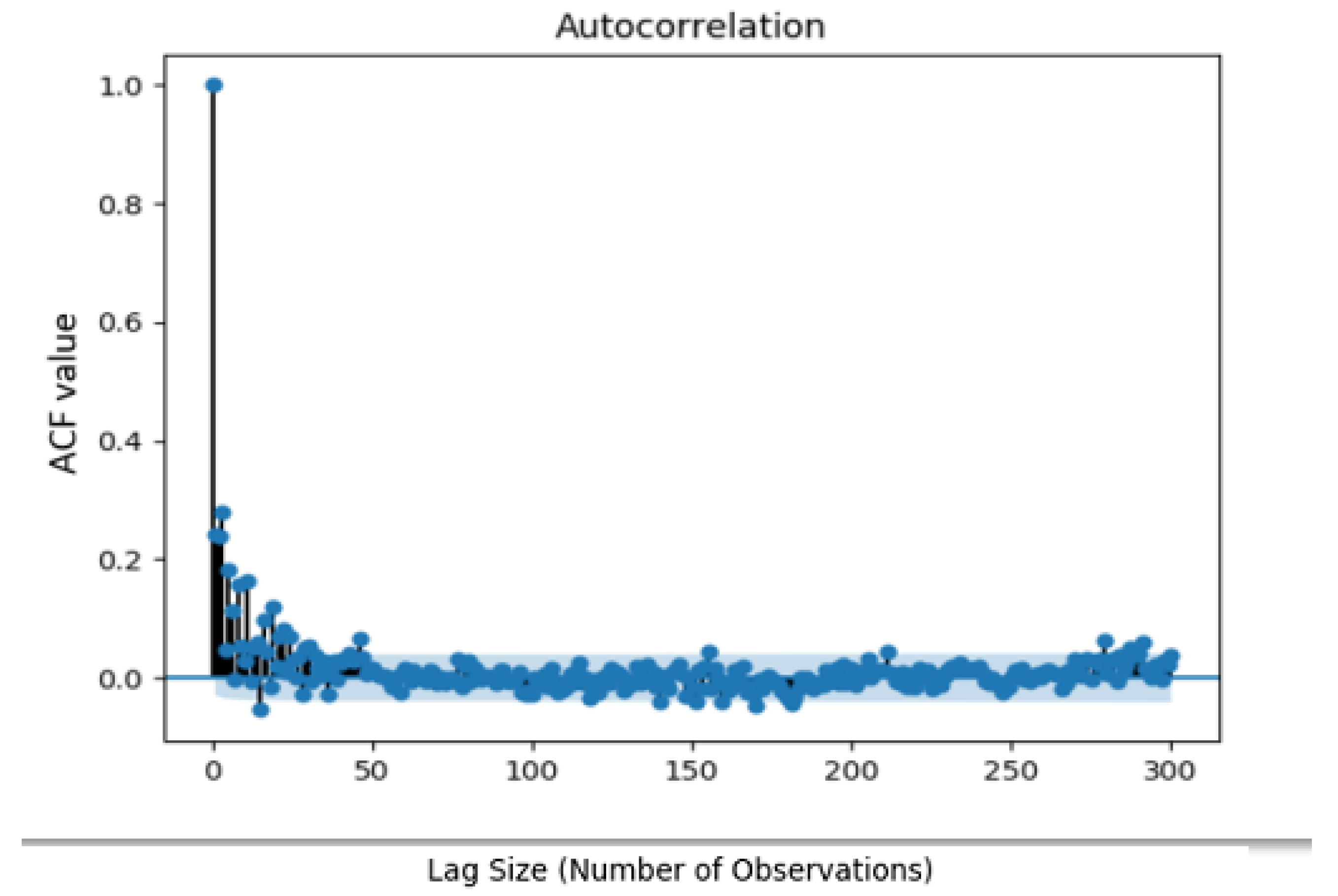
In this paper, the inputs for the neural networks are determined after examining the ACF; the assumption regarding homologous instants is analyzed in the second part of our proposed methodology. Based on this analysis it was derived that the most recent 24-h data exhibit the highest correlation with the forecasts and as such they form the basic input of the proposed methodology. In this way, the day ahead forecast problem is transformed into a uni-step problem. The first part of the analysis deals with the development of the auto-correlation plot of observations starting at time t and for two days duration. Figure 2, Figure 3 and Figure 4 present the correlation analysis and auto-correlation plots for Trento, household and office datasets. The vertical axis shows the ACF value, which ranges from −1 to 1. The horizontal axis of the plot shows the size of the lag between the elements of the time series. For instance, the autocorrelation with lag 4 is the correlation between the time series elements and the corresponding elements observed four periods earlier.
As it can be seen, the highest correlation values are derived at the same time the previous or next day (every 24 h), which confirms the assumption of stationarity of Table 1. According to these results, the highest correlated value, always for after one day, is the:
  • t-144 for Trento
  • t-144 for Household dataset
  • t-288 for the Office dataset
The first step of data transformation is then performed, since these results determine the one of the two dimension of our matrix, namely the columns. The following step is linked with the examination of the datasets in terms of these columns; more precisely we are trying to define a B (batch size) × I (highest correlated value) matrix. Additionally, it is evident that the highest correlated value, determined above will be the input for out model.

3. Results

Batch Size (Hyper-Parameters Tuning) and Data Transformation

Hyper-parameters tuning can enhance the effectiveness of the ANN-based models. The most common method for tuning the model parameters is trial and error. Regarding the number of epochs, there is no general rule or special procedure, since this parameter expresses only the times the dataset is parsed.
On the other hand, the batch size is a much more complex parameter. It determines the number of samples that will be propagated through the network, while the model updates the weights after each propagation instance. The batch size is a very important parameter because it can accelerate or slow down the training process of the model. In this paper, we study the effects that batch size has on the accuracy of the proposed model and an optimal batch size tuning method is proposed. After the correlation analysis is concluded, a time interval is selected which is used as input for our models. Our method ensures that the optimal batch size must correspond to the chosen time interval. When the batch size is randomly selected or the classic trial and error method is employed, the weights are updated in randomly chosen time periods, considering groups of observations that do not match the statistical analysis of the dataset. As a result, the updated weights are incorrect. On the contrary, if the batch size is determined consistently with the chosen time interval, the model reviews a specific time period with proven inclusion of the relevant observations. In this way, the proposed methodology leads to a more efficient tuning process and in most cases to better performances.
Regarding the CNN architecture it comprises of three elements involved in the convolution operation: the input pattern (image), the feature detector (kernel or filter) and the feature map. The feature detector (filter) takes into consideration the parameter that is expressed through its length. In image recognition applications the CNN parses the image into groups determined by the filter length. For example an image of 256 pixels determines a filter length of 256. In our case, as mentioned before, the full time series dataset is separated into smaller groups which express a specific time period with high correlation. Those smaller groups are handled as different images, of different pixel size and the filter length is chosen accordingly. If the statistical analysis concludes that the highest correlated interval is that corresponding to the same time the day before, we have an 1-D image or if it corresponds to that of the same time two days ago, we have a 2-D image of n (observations per day) × 2 (days ago). The n × 2 multiplication implies the resulting filter length following the same reasoning as with the batch size tuning (filter length should be equal to batch size or a derivative of that).
The proposed algorithm was tested on metering data from three different publicly available datasets. For the household use case the measurement site refers to a single family housing with four family members. The sampling period is 10 min. spanning from 12 July 2012 to 26 July 2012. For the office use case the sampling period is 50 min. spanning from 2 July 2014 to 17 July 2014. The energy consumption dataset for Trento is provided by the local energy company, SET, that manages almost the entire electrical network over the Trentino territory [63]. SET uses around 180 primary (medium voltage) distribution lines to bring energy from the national grid (high voltage) to Trentino’s consumers. The dataset was collected from 1 November 2013 to 10 November 2013 over a territory of 6000 km 2 in Northern Italy, the province of Trento. The dataset comprises 50 thousand records for energy consumption and the sampling period consists of 10 min. intervals. The main criterion for the use cases selection was the diversity of the examined datasets. Hence, we test our methodology with different time periods, level/magnitude of demand, consumption patterns and specific characteristics such as demand volatility. By doing so, its applicability is expanded and its advantages are verified. The size of the examined datasets is summarized in Table 3.
For each dataset, the results of the proposed method are compared with the corresponding results from algorithms which are among the most employed methods across literature. To evaluate the forecasting accuracy, we estimate the Mean Absolute Error (MAE) and the Root Mean Square Error (RMSE) [64] as follows:
M A E = i = 1 n | A t F t | n , R M S E = 1 T t = 1 T | A t F t |
where A t are the actuals and F t the corresponding forecasted values. Another metric that is also very popular across literature is the Mean Absolute Percentage Error (MAPE) [65] which is defined as:
M A P E = 100 n i = 1 n | A t F t | A t %
MAPE gives a percentage, so it is useful for comparison purposes. Moreover, percentages are in general, more understandable to people and thus MAPE provides initial information regarding the accuracy of the forecasted time series. Like all percentage errors, MAPE has the advantage of being scale-independent hence it is often employed when we need to compare different time series. On the other hand, MAPE as a percentage, has the disadvantage of being undefined or infinite in case of A t = 0 , or having extreme values when A t is close to zero. Some software tools ignore actual values that are equal to zero, however this aggravates the aforementioned issue since MAPE cannot take into account the forecasts when the actual value is zero. Another issue with percentage metrics is the assumption that A t has a scale based on quantity. However, this is not the case with time series like temperature or energy demand since they are not measuring quantity. Moreover, MAPE value can be over 100% or even negative. A MAPE over 100% means that the errors are “much greater” than the actual values. Based on the above limitations, MAPE, which is a very common accuracy metric, should be used in conjunction with other metrics in order to have a clear indication and better understanding of the examined forecasting models. Because of the nature of load time series and the shortcomings of MAPE, in order to evaluate the performance of our proposed method, we employed only metrics that are related to the absolute values or squared differences of the examined time series, namely Mean Absolute Error (MAE) and Root Mean Square Error (RMSE).
In order to determine the optimal batch sizes for our model, we need to examine the results of the trial and error method applied. The batch sizes examined were multiples of the highest correlated values above. For example for the Trento dataset we experimented with batch sizes of 144, 288 (144 × 2), 432 (144 × 3), but also with a number of randomly chosen ones like 231 or 216 for the office dataset in order to strengthen our assumption. In Figure 5, Figure 6 and Figure 7 the achieved values of MAE and RMSE are presented for different batch sizes for the Trento, household and office datasets respectively. Each dataset is split in two parts, namely the training (80%) and the testing (20%) datasets. Those three datasets present the most interesting scenarios, because the availability of data is very limited and the investigated datasets present higher volatility on their consumption patterns, since they are small scale examples. Therefore, the proposed method offers a solution to the forecasting problem, when data shortage is present and small scale cases are employed.
The household and office datasets are the most challenging ones, since they exhibit low auto-correlation and higher volatility/stochasticity compared to the rest. In the household case, the minimum MAE corresponds to batch sizes (144 observations/day) of 288 and 864 observations respectively (both multiples of 144). Since the minimum RMSE corresponds to a forecasting period of 864 observations, experimental data with different batch sizes indicated that the batch size should be chosen to be 864. Similarly, for the Trento dataset the batch size is chosen at 144 (144 observations per day). The batch size for the office dataset is chosen accordingly. The selected batch sizes for each dataset are summarized in Table 4. The best RMSE and MAE values are derived as a multiple of the number of the batch observations for each dataset. This is derived as a result of the ACF analysis. In Table 5, Table 6 and Table 7, the summarized results of MAE and RMSE for all models and for every dataset are presented.
At this point we have a clear picture of the dataset transformation. As shown in Figure 8, we started from a sequential time series dataset and transformed it accordingly into a matrix. The transformed data are then ready to be fed into the CNN model. If the statistical analysis concludes that the interval with the highest correlation is that corresponding to the same time the day before, we have an 1D image. If it corresponds to that of the same time two days ago, we have a 2D image n (observations per day) × 2 (days ago) image. The n × 2 multiplication implies the resulting filter length following the same reasoning as with the batch size tuning (the filter length should be equal to batch size or to a derivative of that).
The proposed methodology was developed and tested in Python with Keras library the backend of which is Tensorflow. Based on the experimental results shown in Table 5, Table 6 and Table 7 the methodology appears to have good performance and the model selection approach, works satisfactorily even for datasets that exhibit high variability. Our approach was compared against a number of other well reputed AI algorithms such as LSTM, ANN and MLP. These models were chosen due to the fact that are widely accepted in literature and are considered to be suitable for time series forecasting applications, like load forecasting, thus forming a valid candidate for the problem under examination. Regarding ANN we have chosen one hidden layer while for MLP, CNN and LSTM the hidden layers were 5. Such choices were made by trial and error, i.e., adding more hidden layers did not enhance the prediction accuracy. The activation function used was ReLU and the number of epochs was 150 for all models; the optimizer was RMS-Prop and the additional parameters for CNN were the following: size of filter 3 × 3, number of input filters 24, maximum pooling size 3 × 3, and size of strides 1. The batch size was settled based on the methodology explained earlier for all models.
The forecast chosen is the “Day ahead” one as defined by the electricity market. The “Day ahead” market is essential for the operation of the power system since a better forecasting tool means that a market participant (i.e., an aggregator, balance responsible party, local energy market operator etc) will make better choices for the next day operation and will minimize the costs that low-accuracy forecasts would bring (high deviations from the forecasted load would mean higher cost in order to balance the system). In our case study the forecast horizon was restricted by the limited availability of historical data.
In Table 5, Table 6 and Table 7 the results of the investigated models (LSTM, CNN, MLP and ANN) for each one of the datasets are presented. The metrics utilized are the Mean Absolute Error (MAE) and Root Mean Squared Error (RMSE) which are shown in the left column of each table. The CNN-based model outperforms the other ones for all three datasets. CNN achieves better results both in terms of MAE and RMSE, with the only exception being the Trento’s dataset where the RMSE result of MLP is slightly better than that of CNN. The performance of CNN regarding MAE is better than that of MLP and this fact can compensate the RMSE difference while CNN also outperforms the rest of the models. The relatively small RMSE and MAE values justify the claim that the proposed batch size tuning method and the time interval input selection strategy substantially improve the performance of our methodology.
Figure 9, Figure 10 and Figure 11 present the plots of the best forecasts for Trento, household and office datasets. We have chosen to present only the last 20% of all observations from each examined load time series. This was due to two main reasons. Firstly, this part of the dataset is used for testing the algorithm and measuring accuracy of each methodology. Secondly, if we presented all observations and load time series it would be difficult for the reader to drive any conclusions. Also, we present graphically only the CNN algorithm performance since it outperforms all other solutions tested with respect to forecasting accuracy. In Figure 9, Figure 10 and Figure 11 the actual load is depicted with red color line while the blue line represents the forecast for specific observation numbers (X axis). Y corresponds to the total load either actual or forecasted. As shown in Figure 9 and Figure 10 the proposed model follows the actual load successfully with the exception of one spike for each dataset (where our forecast could not predict it successfully). In the household dataset, (in Figure 9) for 1900 observations our model provides a much higher value of the electric load compared to the real one. We observe the same behaviour for the office dataset ( Figure 10). For the Trento dataset (Figure 11), the CNN model performs adequately well and follows quite precisely the value of real, expected load. In general, the results indicate that our model was accurate for all datasets.
Apparently, our model in all three forecasted time series exposes sufficiently good accuracy and follows satisfactorily the actual load time series. Of course, CNN cannot predict the spikes that occur randomly and are the results of sudden disturbances without any pattern and thus very difficult to be predicted. As explained earlier, CNN exploits the temporal stationarity of the load time series, hence it is not possible to predict future observations with high variability. In case of load spikes the temporal stationarity is distorted, therefore CNN cannot provide an accurate prediction.

4. Discussion

In this work we present a methodology that is based on statistical analysis and involves the preprocessing of the time series data before addressing the problem of short term electric load forecasting. The methodology employs statistical learning and proper data transformation in an image-like format in order to benefit from the CNN-based models, which exploit stationarity and time locality. While the superiority and the efficiency of LSTM (based on the importance of the inherent memory in load time series) are widely accepted, we showed that CNN-based models present a credible alternative for short term forecasting problems when compared to LSTM algorithms (leveraging the temporal locality of load time series by analogy with image processing where space locality is exploited). The achieved accuracy, based on MAE and RMSE, indicates that the proposed CNN algorithm’s performance was improved compared to the LSTM model. CNNs seem to achieve better accuracy when we lack of historical data, the scale of the energy entities is small and the forecast horizon is short (day -ahead forecast). Since the efficiency of the LSTM for long term dependencies is unquestionable, a hybrid LSTM-CNN model is worth examining in future research work, especially for multi-step method considerations. The presented methodology performs demand forecasting at low scale level and thus the forecasted time series can be used as input to various energy management algorithms at microgrid or house level, providing a useful tool for optimizing the operation of the energy entities at the grid edge. Even though LSTM is the most common model to tackle the load forecasting problem, we have proven here that CNN can outperform LSTM in cases where the number of the observations and the energy deployment are limited (loads in a household or in a small energy community) and the load patterns change dynamically. We conclude that if AMI and the relevant communications infrastructure exist, the CNN model is more suitable for forecasting loads of a house, office, building or even of an energy community.

Author Contributions

This paper was a collaborative effort among the authors. N.A. and A.M., designed and performed experiments, analysed data, validated the results and co-wrote the paper; A.B., M.B., C.V. and S.D. supervised the research and co-wrote the paper; E.H., A.P. and G.P.P. reviewed the paper. All authors have read and agreed to the published version of the manuscript.

Funding

This research was funded by the EU H2020 research and innovation program under project CROSSBOW—CROSS BOrder management of variable renewable energies and storage units enabling a transnational Wholesale market (Grant No. 773430).

Institutional Review Board Statement

Not applicable.

Informed Consent Statement

Not applicable.

Conflicts of Interest

The authors declare no conflict of interest.

Abbreviations

The following abbreviations are used in this manuscript:
RESRenewable Energy Systems
CNNConvolution Neural Network
LSTMLong Short Term Memory
ARAutoregressive
ARXAutoregressive with Exogenous Variables
ARMAAutoregressive Moving Average
ANNArtificial Neural Network
RNNRecurrent Neural Network
VSTLFVery Short Term Load Forecasting
STLFShort Term Load Forecasting
MTLFMedium Term Load Forecasting
LTLFLong Term Load Forecasting
DERDistributed Energy Resources
DSODistribution System Operator
LVLow Voltage
HVHigh Voltage
PCAPrincipal Component Analysis
MLRMultiple Linear Regression
HEMSHome Energy Management Systems
LEMLocal Energy Markets
THITemperature-Humidity Index
PJMPennsylvania-New Jersey-Maryland
AMIAdvanced Metering Infrastructure
PIPrediction Intervals
LUBELower Upper Bound Estimation
SSASingular Spectrum Analysis
PCPrincipal Components
SVMSupport Vector Machine
WNNWavelet Neural Network
SRWNNSelf-Recurrent Wavelet Neural Network
CRBMConditional Restricted Boltzmann Machine
FCRBMFactored Conditional Restricted Boltzmann Machine
CKDConditional Kernel Density
MLPMultilayer Perceptron
SIANNSpace Invariant Artificial Neural Networks
ReLURectified Linear Unit
ADFAugmented Dickey Fuller
STDstandard deviation
ACFAuto-Correlation Function
MAEMean Absolute Error
RMSERoot Mean Square Error
MAPEMean Absolute Percentage Error

References

  1. Zhang, G.P. Time series forecasting using a hybrid ARIMA and neural network model. Neurocomputing 2003, 50, 159–175. [Google Scholar] [CrossRef]
  2. Papalexopoulos, A.D.; Hesterberg, T.C. A regression-based approach to short-term system load forecasting. IEEE Trans. Power Syst. 1990, 5, 1535–1547. [Google Scholar] [CrossRef]
  3. Papalexopoulos, A.D.; Hao, S.; Peng, T.M. An implementation of a neural network based load forecasting model for the EMS. IEEE Trans. Power Syst. 1994, 9, 1956–1962. [Google Scholar] [CrossRef]
  4. Papalexopoulos, A.D.; Hao, S.; Peng, T.M. Application of neural network technology to short-term system load forecasting. In Proceedings of the Joint International Power Conference Athens Power Tech, Athens, Greece, 5–8 September 1993; Volume 2, pp. 796–800. [Google Scholar]
  5. Chen, B.J.; Chang, M.W. Load forecasting using support vector machines: A study on EUNITE competition 2001. IEEE Trans. Power Syst. 2004, 19, 1821–1830. [Google Scholar] [CrossRef] [Green Version]
  6. Ghelardoni, L.; Ghio, A.; Anguita, D. Energy load forecasting using empirical mode decomposition and support vector regression. IEEE Trans. Smart Grid 2013, 4, 549–556. [Google Scholar] [CrossRef]
  7. Hochreiter, S.; Schmidhuber, J. Long short-term memory. Neural Comput. 1997, 9, 1735–1780. [Google Scholar] [CrossRef]
  8. Zheng, J.; Xu, C.; Zhang, Z.; Li, X. Electric load forecasting in smart grids using long-short-term-memory based recurrent neural network. In Proceedings of the 2017 51st Annual Conference on Information Sciences and Systems (CISS), Baltimore, MD, USA, 22–24 March 2017; pp. 1–6. [Google Scholar]
  9. Giasemidis, G.; Haben, S.; Lee, T.; Singleton, C.; Grindrod, P. A genetic algorithm approach for modelling low voltage network demands. Appl. Energy 2017, 203, 463–473. [Google Scholar] [CrossRef] [Green Version]
  10. Bennett, C.; Stewart, R.A.; Lu, J. Autoregressive with exogenous variables and neural network short-term load forecast models for residential low voltage distribution networks. Energies 2014, 7, 2938–2960. [Google Scholar] [CrossRef]
  11. Bennett, C.J.; Stewart, R.A.; Lu, J.W. Forecasting low voltage distribution network demand profiles using a pattern recognition based expert system. Energy 2014, 67, 200–212. [Google Scholar] [CrossRef] [Green Version]
  12. Høverstad, B.A.; Tidemann, A.; Langseth, H.; Öztürk, P. Short-term load forecasting with seasonal decomposition using evolution for parameter tuning. IEEE Trans. Smart Grid 2015, 6, 1904–1913. [Google Scholar] [CrossRef]
  13. Fan, S.; Hyndman, R.J. Short-term load forecasting based on a semi-parametric additive model. IEEE Trans. Power Syst. 2011, 27, 134–141. [Google Scholar] [CrossRef] [Green Version]
  14. Goude, Y.; Nedellec, R.; Kong, N. Local short and middle term electricity load forecasting with semi-parametric additive models. IEEE Trans. Smart Grid 2013, 5, 440–446. [Google Scholar] [CrossRef]
  15. Ding, N.; Bésanger, Y.; Wurtz, F. Next-day MV/LV substation load forecaster using time series method. Electr. Power Syst. Res. 2015, 119, 345–354. [Google Scholar] [CrossRef]
  16. Ding, N.; Benoit, C.; Foggia, G.; Bésanger, Y.; Wurtz, F. Neural network-based model design for short-term load forecast in distribution systems. IEEE Trans. Power Syst. 2015, 31, 72–81. [Google Scholar] [CrossRef]
  17. Cecati, C.; Citro, C.; Siano, P. Combined operations of renewable energy systems and responsive demand in a smart grid. IEEE Trans. Sustain. Energy 2011, 2, 468–476. [Google Scholar] [CrossRef]
  18. Liu, Y. Continuous dependence for a thermal convection model with temperature-dependent solubility. Appl. Math. Comput. 2017, 308, 18–30. [Google Scholar] [CrossRef]
  19. Rowe, M.; Yunusov, T.; Haben, S.; Holderbaum, W.; Potter, B. The real-time optimisation of DNO owned storage devices on the LV network for peak reduction. Energies 2014, 7, 3537–3560. [Google Scholar] [CrossRef] [Green Version]
  20. Rowe, M.; Yunusov, T.; Haben, S.; Singleton, C.; Holderbaum, W.; Potter, B. A peak reduction scheduling algorithm for storage devices on the low voltage network. IEEE Trans. Smart Grid 2014, 5, 2115–2124. [Google Scholar] [CrossRef]
  21. El-Baz, W.; Tzscheutschler, P. Short-term smart learning electrical load prediction algorithm for home energy management systems. Appl. Energy 2015, 147, 10–19. [Google Scholar] [CrossRef]
  22. Keerthisinghe, C.; Verbič, G.; Chapman, A.C. A fast technique for smart home management: ADP with temporal difference learning. IEEE Trans. Smart Grid 2016, 9, 3291–3303. [Google Scholar] [CrossRef]
  23. Pratt, A.; Krishnamurthy, D.; Ruth, M.; Wu, H.; Lunacek, M.; Vaynshenk, P. Transactive home energy management systems: The impact of their proliferation on the electric grid. IEEE Electrif. Mag. 2016, 4, 8–14. [Google Scholar] [CrossRef]
  24. Morstyn, T.; Farrell, N.; Darby, S.J.; McCulloch, M.D. Using peer-to-peer energy-trading platforms to incentivize prosumers to form federated power plants. Nat. Energy 2018, 3, 94–101. [Google Scholar] [CrossRef]
  25. Hong, T.; Xie, J.; Black, J. Global energy forecasting competition 2017: Hierarchical probabilistic load forecasting. Int. J. Forecast. 2019, 35, 1389–1399. [Google Scholar] [CrossRef]
  26. Haben, S.; Ward, J.; Greetham, D.V.; Singleton, C.; Grindrod, P. A new error measure for forecasts of household-level, high resolution electrical energy consumption. Int. J. Forecast. 2014, 30, 246–256. [Google Scholar] [CrossRef] [Green Version]
  27. Sousa, J.M.; Neves, L.M.; Jorge, H.M. Short-term load forecasting using information obtained from low voltage load profiles. In Proceedings of the 2009 International Conference on Power Engineering, Energy and Electrical Drives, Lisbon, Portugal, 18–20 March 2009; pp. 655–660. [Google Scholar]
  28. Veit, A.; Goebel, C.; Tidke, R.; Doblander, C.; Jacobsen, H.A. Household electricity demand forecasting: Benchmarking state-of-the-art methods. In Proceedings of the 5th International Conference on Future Energy Systems, Cambridge, UK, 11–13 June 2014; pp. 233–234. [Google Scholar]
  29. Chitsaz, H.; Shaker, H.; Zareipour, H.; Wood, D.; Amjady, N. Short-term electricity load forecasting of buildings in microgrids. Energy Build. 2015, 99, 50–60. [Google Scholar] [CrossRef]
  30. Ghofrani, M.; Hassanzadeh, M.; Etezadi-Amoli, M.; Fadali, M.S. Smart meter based short-term load forecasting for residential customers. In Proceedings of the 2011 North American Power Symposium, Boston, MA, USA, 4–6 August 2011; pp. 1–5. [Google Scholar]
  31. Yu, C.N.; Mirowski, P.; Ho, T.K. A sparse coding approach to household electricity demand forecasting in smart grids. IEEE Trans. Smart Grid 2016, 8, 738–748. [Google Scholar] [CrossRef]
  32. Xie, J.; Hong, T.; Stroud, J. Long-term retail energy forecasting with consideration of residential customer attrition. IEEE Trans. Smart Grid 2015, 6, 2245–2252. [Google Scholar] [CrossRef]
  33. Vercamer, D.; Steurtewagen, B.; Van den Poel, D.; Vermeulen, F. Predicting consumer load profiles using commercial and open data. IEEE Trans. Power Syst. 2015, 31, 3693–3701. [Google Scholar] [CrossRef]
  34. Xie, J.; Chen, Y.; Hong, T.; Laing, T.D. Relative humidity for load forecasting models. IEEE Trans. Smart Grid 2016, 9, 191–198. [Google Scholar] [CrossRef]
  35. Sun, X.; Luh, P.B.; Cheung, K.W.; Guan, W.; Michel, L.D.; Venkata, S.; Miller, M.T. An efficient approach to short-term load forecasting at the distribution level. IEEE Trans. Power Syst. 2015, 31, 2526–2537. [Google Scholar] [CrossRef]
  36. Borges, C.E.; Penya, Y.K.; Fernandez, I. Evaluating combined load forecasting in large power systems and smart grids. IEEE Trans. Ind. Inform. 2012, 9, 1570–1577. [Google Scholar] [CrossRef]
  37. Marinescu, A.; Harris, C.; Dusparic, I.; Clarke, S.; Cahill, V. Residential electrical demand forecasting in very small scale: An evaluation of forecasting methods. In Proceedings of the 2013 2nd International Workshop on Software Engineering Challenges for the Smart Grid (SE4SG), San Francisco, CA, USA, 18 May 2013; pp. 25–32. [Google Scholar]
  38. Quilumba, F.L.; Lee, W.J.; Huang, H.; Wang, D.Y.; Szabados, R.L. Using smart meter data to improve the accuracy of intraday load forecasting considering customer behavior similarities. IEEE Trans. Smart Grid 2014, 6, 911–918. [Google Scholar] [CrossRef]
  39. Quan, H.; Srinivasan, D.; Khosravi, A. Short-term load and wind power forecasting using neural network-based prediction intervals. IEEE Trans. Neural Netw. Learn. Syst. 2013, 25, 303–315. [Google Scholar] [CrossRef] [PubMed]
  40. Papaioannou, G.P.; Dikaiakos, C.; Dramountanis, A.; Papaioannou, P.G. Analysis and modeling for short-to medium-term load forecasting using a hybrid manifold learning principal component model and comparison with classical statistical models (SARIMAX, Exponential Smoothing) and artificial intelligence models (ANN, SVM): The case of Greek electricity market. Energies 2016, 9, 635. [Google Scholar]
  41. Edwards, R.E.; New, J.; Parker, L.E. Predicting future hourly residential electrical consumption: A machine learning case study. Energy Build. 2012, 49, 591–603. [Google Scholar] [CrossRef]
  42. Shi, H.; Xu, M.; Li, R. Deep learning for household load forecasting—A novel pooling deep RNN. IEEE Trans. Smart Grid 2017, 9, 5271–5280. [Google Scholar] [CrossRef]
  43. Tascikaraoglu, A.; Sanandaji, B.M. Short-term residential electric load forecasting: A compressive spatio-temporal approach. Energy Build. 2016, 111, 380–392. [Google Scholar] [CrossRef]
  44. Kumar, R.; Aggarwal, R.; Sharma, J. Energy analysis of a building using artificial neural network: A review. Energy Build. 2013, 65, 352–358. [Google Scholar] [CrossRef]
  45. Kong, W.; Dong, Z.Y.; Hill, D.J.; Luo, F.; Xu, Y. Short-term residential load forecasting based on resident behaviour learning. IEEE Trans. Power Syst. 2017, 33, 1087–1088. [Google Scholar] [CrossRef]
  46. Keren, G.; Schuller, B. Convolutional RNN: An enhanced model for extracting features from sequential data. In Proceedings of the 2016 International Joint Conference on Neural Networks (IJCNN), Vancouver, BC, Canada, 24–29 July 2016; pp. 3412–3419. [Google Scholar]
  47. Acharya, S.K.; Wi, Y.M.; Lee, J. Short-Term Load Forecasting for a Single Household Based on Convolution Neural Networks Using Data Augmentation. Energies 2019, 12, 3560. [Google Scholar] [CrossRef] [Green Version]
  48. Canizes, B.; Silva, M.; Faria, P.; Ramos, S.; Vale, Z. Resource scheduling in residential microgrids considering energy selling to external players. In Proceedings of the 2015 Clemson University Power Systems Conference (PSC), Clemson, SC, USA, 10–13 March 2015; pp. 1–7. [Google Scholar]
  49. Almabdy, S.; Elrefaei, L. Deep convolutional neural network-based approaches for face recognition. Appl. Sci. 2019, 9, 4397. [Google Scholar] [CrossRef] [Green Version]
  50. Li, L.; Ota, K.; Dong, M. Everything is image: CNN-based short-term electrical load forecasting for smart grid. In Proceedings of the 2017 14th International Symposium on Pervasive Systems, Algorithms and Networks & 2017 11th International Conference on Frontier of Computer Science and Technology & 2017 Third International Symposium of Creative Computing (ISPAN-FCST-ISCC), Exeter, UK, 21–23 June 2017; pp. 344–351. [Google Scholar]
  51. Zhang, W. Shift-invariant pattern recognition neural network and its optical architecture. In Proceedings of the Annual Conference of the Japan Society of Applied Physics, Keio Plaza Hotel, Tokyo, Japan, 24–26 August 1988. [Google Scholar]
  52. Zhang, W.; Itoh, K.; Tanida, J.; Ichioka, Y. Parallel distributed processing model with local space-invariant interconnections and its optical architecture. Appl. Opt. 1990, 29, 4790–4797. [Google Scholar] [CrossRef] [PubMed]
  53. Saha, S. A Comprehensive Guide to Convolutional Neural Networks—the ELI5 Way. 2018. Available online: https://towardsdatascience.com/a-comprehensive-guide-to-convolutional-neural-networks-the-eli5-way-3bd2b1164a53 (accessed on 16 December 2016).
  54. LeCun, Y.; Bengio, Y.; Hinton, G. Deep learning. Nature 2015, 521, 436–444. [Google Scholar] [CrossRef] [PubMed]
  55. LeCun, Y.; Kavukcuoglu, K.; Farabet, C. Convolutional networks and applications in vision. In Proceedings of the 2010 IEEE International Symposium on Circuits and Systems, Paris, France, 30 May–2 June 2010; pp. 253–256. [Google Scholar]
  56. LeCun, Y.; Boser, B.; Denker, J.S.; Henderson, D.; Howard, R.E.; Hubbard, W.; Jackel, L.D. Backpropagation applied to handwritten zip code recognition. Neural Comput. 1989, 1, 541–551. [Google Scholar] [CrossRef]
  57. Fukushima, K.; Miyake, S.; Ito, T. Neocognitron: A neural network model for a mechanism of visual pattern recognition. IEEE Trans. Syst. Man. Cybern. 1983, 5, 826–834. [Google Scholar] [CrossRef]
  58. Krizhevsky, A.; Sutskever, I.; Hinton, G.E. Imagenet classification with deep convolutional neural networks. In (NIPS’12), Proceedings of the 25th International Conference on Neural Information Processing Systems—Volume 1, Lake Tahoe, Nevada, 3–8 December 2012; Curran Associates Inc.: Red Hook, NY, USA, 2012; pp. 1097–1105. [Google Scholar]
  59. Simonyan, K.; Zisserman, A. Very deep convolutional networks for large-scale image recognition. arXiv 2014, arXiv:1409.1556. [Google Scholar]
  60. Deng, L.; Yu, D. Deep learning: Methods and applications. Found. Trends Signal Process. 2014, 7, 197–387. [Google Scholar] [CrossRef] [Green Version]
  61. Mills, T.C.; Mills, T.C. Time Series Techniques for Economists; Cambridge University Press: Cambridge, UK, 1991. [Google Scholar]
  62. Greene, W.H. LIMDEP. New York: Econometric Software. _. 1990. Econometric Analysis; MacMillan: New York, NY, USA, 1989. [Google Scholar]
  63. Barlacchi, G.; De Nadai, M.; Larcher, R.; Casella, A.; Chitic, C.; Torrisi, G.; Antonelli, F.; Vespignani, A.; Pentland, A.; Lepri, B. A multi-source dataset of urban life in the city of Milan and the Province of Trentino. Sci. Data 2015, 2, 1–15. [Google Scholar] [CrossRef] [Green Version]
  64. Willmott, C.J.; Matsuura, K. Advantages of the mean absolute error (MAE) over the root mean square error (RMSE) in assessing average model performance. Clim. Res. 2005, 30, 79–82. [Google Scholar] [CrossRef]
  65. De Myttenaere, A.; Golden, B.; Le Grand, B.; Rossi, F. Mean absolute percentage error for regression models. Neurocomputing 2016, 192, 38–48. [Google Scholar] [CrossRef] [Green Version]
Figure 1. CNN architecture [53].
Applsci 11 00158 g001
Figure 2. Autocorrelation plot for Trento data. The vertical axis shows the ACF value. The horizontal axis of the plot shows the size of the lag between the elements of the time series.
Applsci 11 00158 g002
Figure 3. Autocorrelation plot for the single household data. The vertical axis shows the ACF value. The horizontal axis of the plot shows the size of the lag between the elements of the time series.
Applsci 11 00158 g003
Figure 4. Autocorrelation plot for the office data. The vertical axis shows the ACF value. The horizontal axis of the plot shows the size of the lag between the elements of the time series.
Applsci 11 00158 g004
Figure 5. Metrics for the Household case: Household MAE and Household RMSE.
Applsci 11 00158 g005
Figure 6. Metrics for the Office case: Office MAE and Office RMSE.
Applsci 11 00158 g006
Figure 7. Metrics for Trento case: Trento MAE and Trento RMSE.
Applsci 11 00158 g007
Figure 8. Data transformation.
Applsci 11 00158 g008
Figure 9. Actual and forecasted load (household). The actual load is depicted with red color and the forecasted time series with blue color.
Applsci 11 00158 g009
Figure 10. Actual and forecasted load (office). The actual load is depicted with red color and the forecasted time series with blue color.
Applsci 11 00158 g010
Figure 11. Actual and forecasted load (Trento). The actual load is depicted with red color and the forecasted time series with blue color.
Applsci 11 00158 g011
Table 1. Stationarity analysis results.
DatasetTrentoHouseholdOffice
Mean 144.58235.731.25
Mean 261.43215.451.15
STD 118.97298.701.30
STD 217.14218.621.07
StationaryNONOYES
Table 2. ADF Test results.
Datasetp-Value (ADF Test)ADFStationary
Trento0.01−3.40YES
Household≪0.01−18.4YES
Table 3. Datasets Results.
DatasetTrentoHouseholdOffice
Size (days)91415
Dataset size (observations)129620164320
Table 4. Parameters Selection.
DatasetTrentoHouseholdOffice
Batch size144 (144 × 1)864 (144 × 6)288 (288 × 1)
Inputt-144t-144t-288
Table 5. Results (Trento).
ModelsLSTMCNNMLPANN
MAE4.583.935.277.58
RMSE5.34.674.566.63
Table 6. Results (Household).
ModelsLSTMCNNMLPANN
MAE0.660.550.580.78
RMSE1.10.930.961.25
Table 7. Results (Office).
ModelsLSTMCNNMLPANN
MAE114.8108.29140.55172.38
RMSE189.38180.54224.96236
Publisher’s Note: MDPI stays neutral with regard to jurisdictional claims in published maps and institutional affiliations.

