A Proposal and Analysis of New Realistic Sets of Benchmark Instances for Vehicle Routing Problems with Asymmetric Costs

Abstract

Despite their importance, relatively little attention has been paid to vehicle routing problems with asymmetric costs (ACVRPs), or their benchmark instances. Taking advantage of recent advances in map application programming interfaces (APIs) and shared spatial data, this paper proposes new realistic sets of ACVRP benchmark instances. The spatial data of urban distribution centers, postal hubs, large shopping malls, residential complexes, restaurant businesses and convenience stores are used. To create distance and time matrices, the T map API, one of the most frequently used real time path analysis and distance measurement tools in Korea, is used. This paper also analyzes some important issues prevailing in urban transportation environments. These include the challenges of accounting for the frequency and distance in which air travel differs from reality when measuring closeness, the differences in distance and time for outgoing and return trips, and the rough conversion ratios from air distance to road distance and to road time. This paper contributes to the research community by providing more realistic ACVRP benchmark instances that reflect urban transportation environments. In addition, the cost matrix analyses provide insights into the behaviors of urban road networks.

1. Introduction

Generally, vehicle routing problems (VRPs) involve a homogeneous fleet of vehicles with a fixed capacity to serve a set of customers from a single depot. All vehicles must depart from and return to the depot. Restrictions such as route lengths or time limits will constrain the distance traveled by the vehicles. The goal is to assign a sequence of deliveries to each vehicle so that service can be provided to all customers while minimizing the total distance traveled or the total time consumed by the fleet. The standard VRP is often referred to as a capacitated vehicle routing problem (CVRP). VRP variations exist, including the multi-depot vehicle routing problem (MVRP), in which vehicles depart from multiple depots, and the open vehicle routing problem (OVRP), in which vehicles do not return to the depot. More detailed lists and descriptions can be found in [1,2].

Relatively little attention or effort has been paid to the creation of benchmark instances for VRPs with asymmetric costs, or asymmetric cost VRPs (ACVRPs). For an ACVRP, a number of old small-sized benchmark instances exist, but they are not able to adequately reflect real-world problems. There are also many new larger-sized instances that lack rationale for the methods used in their creation. This lack can, in part, be explained by the difficulty in obtaining the exact road distance or time from all nodes to other nodes. However, recent advances in technology have made it possible to clear this hurdle. Now with the advance of map service providers and their efficient application programming interfaces (APIs), the distance or time of paths can be estimated very accurately.

As illustrated in Figure 1, map APIs can provide precise costs between nodes. The figure explains why the real road distances from map APIs should be used instead of air distances or the straight-line distances between coordinates. In Figure 1a, A′ exemplifies the closest node from Node A in the road networks of a map service provider. The air distance from A to B may be larger than the air distance from A to C, but the road distance from A to B (blue solid line) is much larger than the road distance from A to C (red dotted line). Figure 1b shows that outbound and return distances can differ by a significant margin. With air distance, the difference of cost from A to B (blue solid line) and from B to A (red dotted line) cannot be properly considered.

Travel costs are asymmetric in real-world settings. That is, the cost of traveling from one node to another node, and the cost of the return trip, can vary. This simple but important fact has naively been ignored in VRP research and operations.

The cost differences may be too small to be concerned with in cases where obstacles and road directions are less important. This would include long-haul or truck-line transportation. However, on a scale of goods distribution or last-mile deliveries where customer nodes are densely populated, the cost differences of outbound and return trips are too large to be ignored. Taking the asymmetry into account has become not only possible, but also significant. Solving a VRP with air distances and then applying asymmetric road distances has been reported to be suboptimal by almost five percent [3]. The asymmetry has a large effect over the solution methods and quality in VRPs, and this dynamic should be considered when proposing and improving routing algorithms [4]. The research community needs properly designed and realistic ACVRP benchmark instances when developing these algorithms.

This paper supplements the pool of ACVRP benchmarks with more realistic instances. An increasing number of governmental authorities are now operating public data portals, which is also true in Korea. Various types and abundant sizes of data have become readily accessible to the public. The provided instances are derived from the actual geographic data of urban distribution centers (UDCs), regional hubs for postal services, shopping malls, restaurant businesses, residential facilities and convenience stores in the cities of Seoul and Busan, Korea. The real road distance and road time matrices are built using the T map API. T map, owned by SK Telecom, is the most accurate and the most used map service provider in Korea [5,6].

Using the realistically created road distance and road time matrices, this paper reveals the frequency and distances by which the air distance differs from reality. The findings not only explain the necessities of using map APIs when planning deliveries in urban areas, but also provide insights and guidelines for urban and logistics planners.

The rest of the paper is organized as follows. Section 2 provides a literature review and background information. The ACVRP and its existing benchmark instances are summarized, and a recent trend of including the use of map APIs in solving VRP variants is reviewed. In Section 3, first, the need for new realistic benchmark instances is explained, and then methods, reasons and sources for the new data sets are presented. Using the road distance and road time in the new benchmark sets, Section 4 conducts an analysis on three issues: how air distance can be deceiving when measuring costs, how outgoing and return trips differ in cost, and the magnitude in which road distances exceed air distances on average. Section 5 provides some possible limitations on the proposal and analysis of the new benchmarks. Section 6 concludes the paper with a summary and suggestions on future research.

2. Literature Review

2.1. VRP with Asymmetric Costs

The rich VRP [7] was developed to tackle multiple real-life VRP considerations, including uncertainty, the use of heterogeneous fleets, and realistic time or distance factors. One important branch of the rich VRP is the VRP with asymmetric costs. Extensive studies regarding the effect of asymmetric costs on the traveling salesman problem (TSP) [8] and VRP [4] argue that asymmetry has a large effect over the solution methods and quality, and that asymmetry should be considered when proposing and improving routing algorithms. Lead and founder of OptaPlanner [3], Geoffrey De Smet, reported that solving a VRP with air distances and then applying asymmetric road distances was suboptimal by almost five percent. Despite the inevitability and significance of asymmetry, insufficient attention has been paid to ACVRPs in the existing literature [9,10].

A number of exact algorithms for ACVRPs were addressed in [11,12]. Subsequently, researchers have focused on numerous ACVRP variants, including backhaul [13], simultaneous pickup and delivery [14], heterogeneous fleets [10], exclusive lanes [15], stochastic demands [16], and time windows [17]. However, few researchers paid attention to the classical ACVRP itself. This was not because the scientific community had conquered the problem. Rather, this was due to the fact that the ACVRP lacks benchmark instances or published best-known solutions.

A well-known set of benchmark instances was provided in Fischetti’s work [18], which included eight instances with the number of nodes, or the dimension, ranging from 34 to 74. By modifying the original vehicle capacity of 1000 to different levels, instances grew in terms of population [19], but not in terms of dimension. The small-sized ACVRP instances were not sufficient to test state-of-the-art algorithms. A breakthrough was achieved by a study that evaluated the effects of asymmetry in VRPs [4]. The research provided 1350 freely available asymmetric road distance instances with dimensions ranging from 50 to 500 [20]. The real road distances were obtained using the Google Maps API [21]. Each instance was provided with two different levels of vehicle capacity, which made for a total of 2700 instances. Of course, 2700 symmetric instances were also prepared to match the asymmetric instances. Although they solved all instances using well-known heuristics, the best solutions found were not reported. This was because the focus of the research was on analyzing the effects of asymmetry, not on proposing an efficient routing algorithm. Other than the research carried out by Herrero [10], in which 20 instances with dimensions of 50 and 100 were deployed, the new instances remain untapped. OptaPlanner has also created benchmark instances for ACVRPs that are available online [22]. The OpenStreetMap API [23] was used to acquire real road distances and times. For each category of asymmetric road distances, asymmetric road times, and symmetric air distances, five instances sized from 50 to 2750 were provided, none of which had any record of the optimal or best-known solutions.

2.2. VRP and Map APIs

Apart from endeavoring to create benchmark instances, recent VRP studies have also employed map APIs to produce more realistic and practical solutions. For instance, utilizing the Google Maps API, a dynamic vehicle routing system based on online map service was designed [24]. The map service was able to help accommodate dynamic customer demands and traffic information in the research. In addition, a study on school bus routing and scheduling, which could be treated as a multi-objective VRP, used the map service to obtain economical routing results that met time window constraints [25]. The OpenStreetMap API has been another option for accurate travel time estimations. A case study on the development of a commercial dynamic vehicle routing system made good use of the map service [26].

With accumulated data and knowledge, it is common that local map service companies provide the best quality information for their region. For example, Baidu’s map service [27] would be the most appropriate choice in China. Many studies on VRP variants, including green VRPs [28], multi-depot VRPs with shared resources [29], or VRPs for emergency cold chain logistics [30], have been carried out using the map service in China. In case of Korea, T map, owned by SK Telecom, is the most popular and the most used map service in the country. Holding the largest telecommunications market share in the country, the map service has over ten thousand users [5]. In Seoul, Korea, the T map API service reflects actual travel patterns and travel times better than foreign map APIs [6]. However, as of writing, no cases could be found in the VRP literature that incorporated T map.

3. New Sets of Benchmark Instances for the ACVRP

3.1. Existing Benchmark Instances

To conveniently represent the sets of benchmark instances from previous studies, they are named after their authors. In this paper, they will be referred to as Fischetti instances [18], De Smet instances [22], and Rodríguez instances [20]. Before looking into each set of instances in detail, the point is made that they were created in Western and Southern European countries. It would be both interesting and necessary to develop benchmark instances in Asian cities, including Seoul and Busan, with the aim of complementing the knowledge and experience that, until now, has been developed from European cities. Compared to Europe, Asian cities can have different population densities, road network systems, urban planning, or periods of development, resulting in distinguished urban structures.

Fischetti instances are small in their number (the number of instances) and dimension (the number of nodes). The instance sets are derived from real-life pharmaceutical product delivery problems in downtown Bologna, Italy. There are eight instances in the set. Including 38 pharmacies, 32 herbalist shops, and a depot, the maximum dimension in the set is 71. The dimensional sizes in the set would not be sufficient for testing cutting-edge VRP solving algorithms. It is also noted that the instances were from the 1990s. The costs were obtained from solving multiple shortest path problems on the road network and not from map APIs.

De Smet instances are not specifically designed for the ACVRP. After excluding instances for multi-depot or time window problems, five ACVRP instances are available. Each instance is provided with two matrix options, road distance and road time, which make a total of ten instances for the set. The dimensions range from 50 to 2750. The fact that the maximum dimension is very large makes these instances a viable alternative for testing state-of-the-art VRP algorithms. However, the customer nodes are not exactly from real-life problems. Administrative locations for cities, towns, and sub-towns are used as the node coordinates.

Rodríguez instances are overwhelming in number. The set consists of 1350 instances. For each instance, two settings—the requested demand quantity from the customers and the vehicle capacity—are provided. This brings the aggregate number to 2700. The number of customer nodes is set from small to large in size (from 50 to 500). The cost matrix is only in road distance. The customer locations are generated based on random, grid and radial distributions, as shown in Figure 2. Using geographic information system (GIS) functions, the generated locations are corrected to the nearest accessible location in the network. Even though the authors made significant efforts to include realistic perspectives, it is arguable that the locations are rather randomly placed, not exactly reflecting realistic circumstances.

3.2. New Benchmark Instances

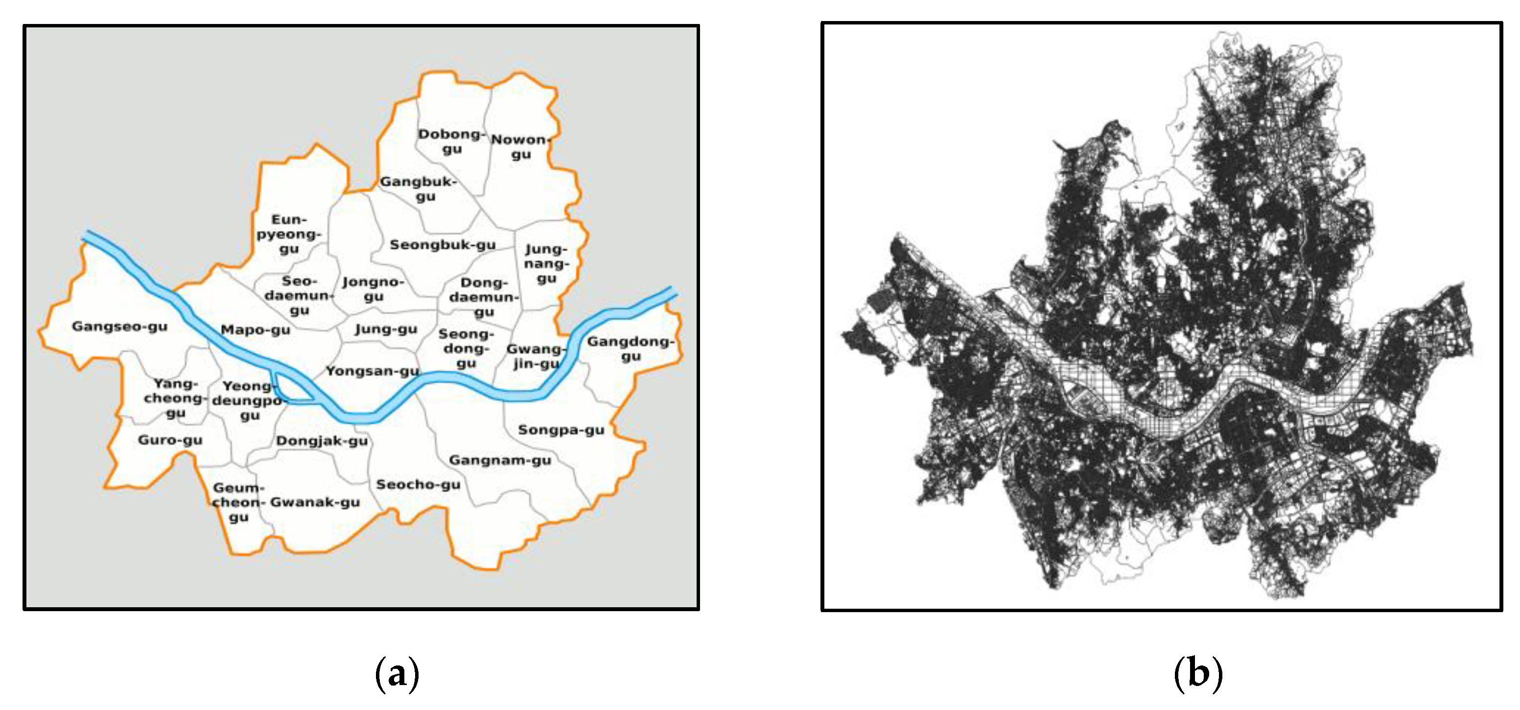
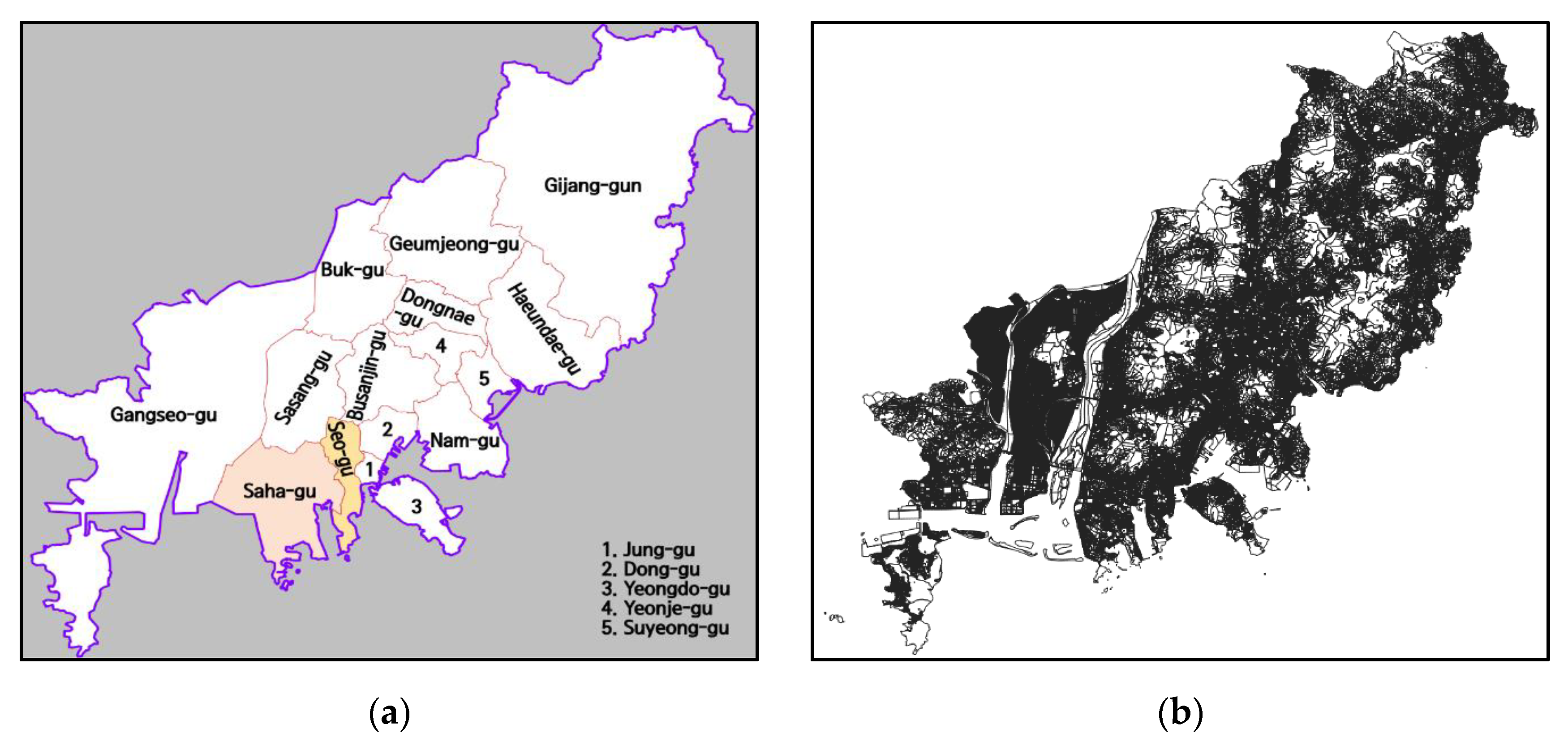
None of the existing sets of ACVRP benchmark instances satisfy all of the following qualities at the same time: (i) it is large in number, (ii) it includes instances that are large in dimension, (iii) its locations carefully reflect the reality of urban transportation, and (iv) it includes both distance and time matrices. These four major requirements should be included in newly created benchmark instances. Of note, having a time matrix for cost considerations is important since labor costs are the dominant factor in delivery operation costs, accounting for over 80 percent [31]. The new and freely available instances are posted online in the Mendeley data repository [32].

3.2.1. Territory

Two cities in Korea, Seoul and Busan, are selected as territorial bases for the benchmark instances. The major two cities have the largest populations in the country. Seoul has ten million inhabitants, with a density of 16,523 persons per km². Busan has three and a half million, with a density of 4546 persons per km². The two cities are selected to represent urban logistics environments. Their geographic shapes are shown in Figure 3 and Figure 4.

3.2.2. Depot Locations

In the two cities, depot locations are based on UDCs, hub terminals for national postal services, and some large shopping malls. Deliveries starting from the UDCs or postal hubs are reasonable from a logistics point of view, but setting a shopping mall as depot location may seem contrary. However, this reflects the booming demand in last-mile delivery services, which have increased significantly during the COVID-19 pandemic.

The spatial data for the depot locations are obtained from shared data produced by various public institutions in Korea. Locations for UDCs, postal hub terminals and mega shopping malls are shared by the Korean National Logistics Information Center. Spatial data for postal hub centers and shopping malls are from the Korean Ministry of Science and ICT (Information and Communications Technology) and the Korean Land and Geospatial Informatrix Corporation, respectively.

In Figure 5 and Figure 6, large markets are denoted as blue squares. Among them, one for Seoul and one for Busan are randomly chosen for the benchmark creation. Similarly, for the UDCs and postal hubs, one of each are selected for the Seoul instances, and one of each is selected for the Busan instances.

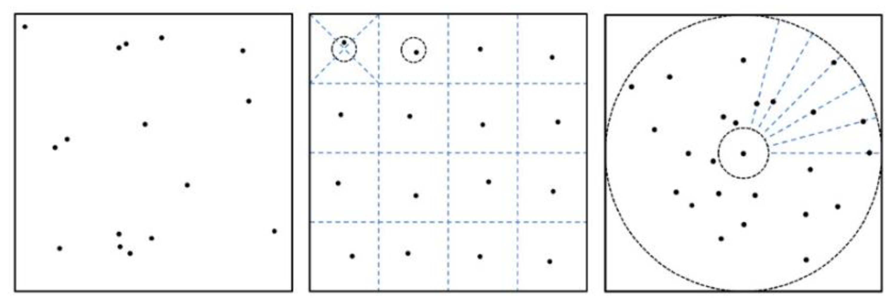
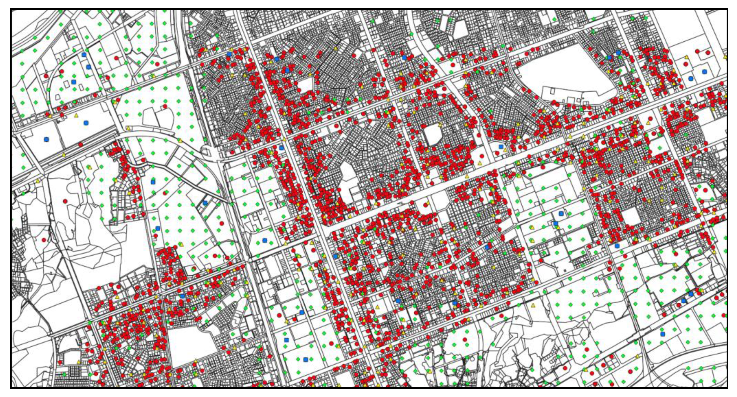
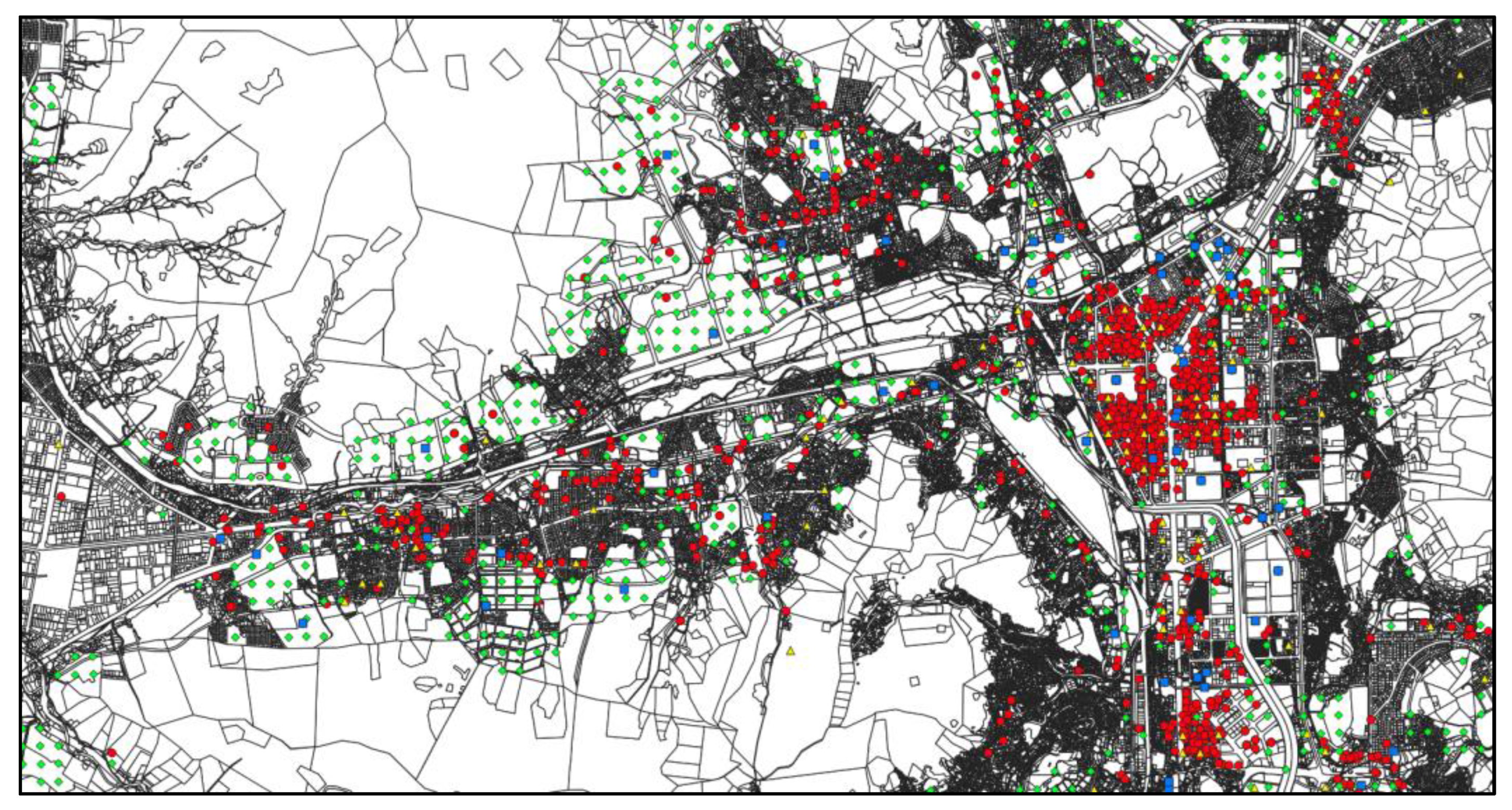
3.2.3. Customer Locations

The spatial data for customer locations are acquired from the National Spatial Data Infrastructure Portal run by the Korean Ministry of Land, Infrastructure, and Transport. The locations are restaurant businesses, residentials complexes, and convenience stores, which are, respectively, marked as red circles, green diamonds, and yellow triangles in Figure 5 and Figure 6.

The figures are worth taking note of for two reasons. First, it is observed that residential areas and business areas are separated. Second, the entities of interest are geographically clustered. This can be attributed to the first note, or the fact that there are more data-sparse areas, as illustrated in Figure 6, mostly because of forested areas, fields, or farmlands.

3.2.4. Vehicle Capacities

In the distribution of goods in the country, 1-ton trucks and 2.5-ton trucks are used most frequently. A 1-ton truck, as the name itself implies, can carry one ton of cargo at maximum. When it comes to volume, it can hold up to seven cubic meters of cargo. On a 2.5-ton truck, about eighteen cubic meters of cargo can be loaded. The load factor, or the ratio of the truck’s used capacity to available capacity, for 1-ton trucks and 2.5-ton trucks are reported to be around 70 percent [35] by the Korea Ministry of Land, Infrastructure and Transport.

In urban freight distribution, the volume of packages can be the major limiting factor [36]. Accordingly, vehicle capacities are assumed to be the volume capacities in the new sets of benchmark instances. For 1-ton trucks and 2.5-ton trucks, the capacities are set to be 5 and 12.5 cubic meters, respectively.

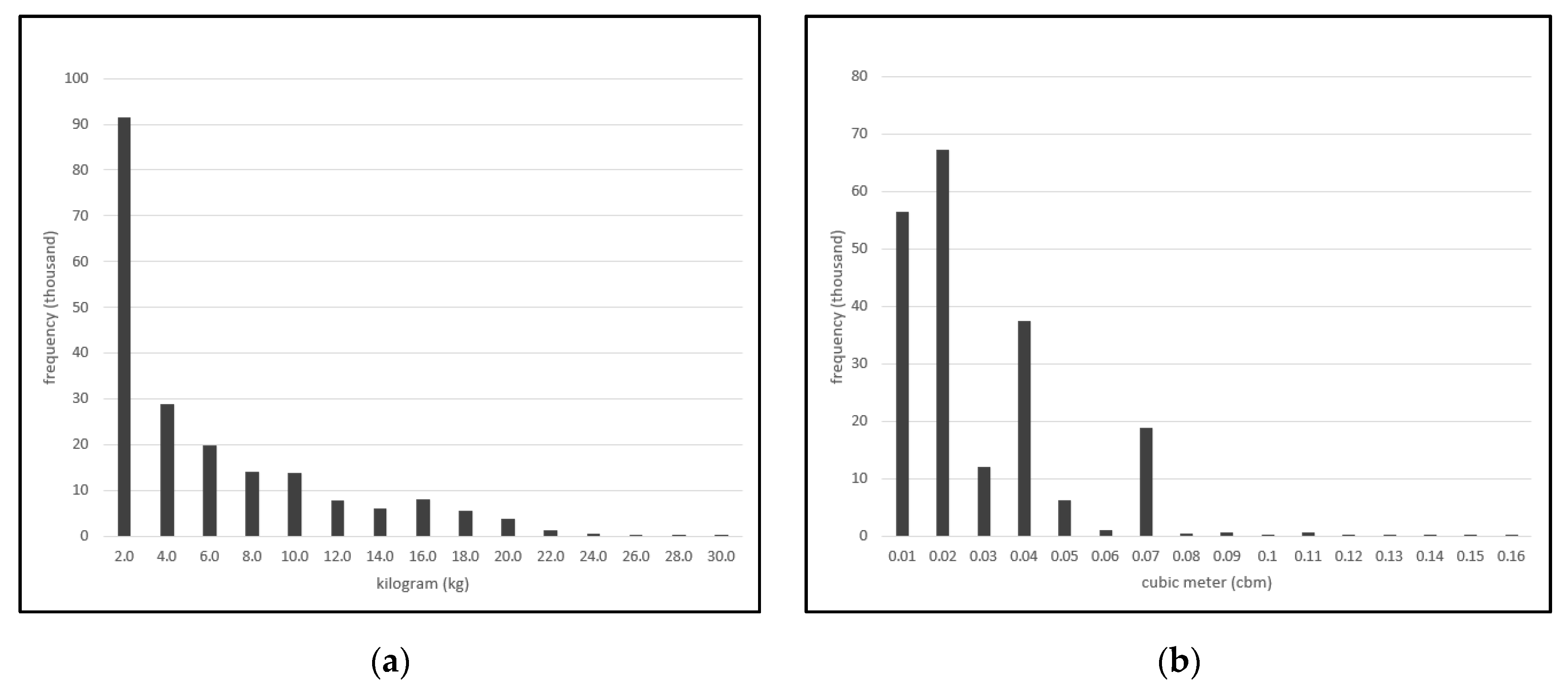
3.2.5. Weight and Volume Per Delivery

As reported by the Korean Ministry of Science and ICT, Korea Post’s market share on parcel delivery exceeds 50 percent. From Korea Post, 200,000 records of delivery weight and volume have been shared to the public. Each customer delivery demand, whether it is a boxed package or a bag of rice, includes weight and volume attributes, and Figure 7 represents the empirical distribution of weight and volume. The volume for each delivery is set using this information, or with multiples of the values.

3.2.6. Dimension and Distance from Depot

VRP dimension represents the number of nodes included in the problem. The nodes are the depot and the customer locations. The dimension of the benchmark sets ranges from 50 to 500. In the benchmark sets, the dimension increases along with the maximum distance from the depot. For example, an instance with a dimension of 250 is created using entities within 5 km from the depot, while an instance with a dimension of 500 is created using the constraint of 10 km.

3.2.7. Cost Matrix

The new benchmark instances are based on the T map API’s road distances and road times. As illustrated in Figure 1, using road distance from map APIs is more accurate than using air distance and can reflect the asymmetric costs between nodes. Of note, having a time matrix rather than just a distance matrix is crucial since labor costs are the major factor in logistics costs.

Table 1. Cost matrix examples: (a) Air distance; (b) road distance; (c) road time.

		To
		Distance between Coordinates						Map API Used
		(a) Air Distance (Meters)						(b) Road Distance (Meters)						(c) Road Time (Seconds)
		A	B	C	D	E	F	A	B	C	D	E	F	A	B	C	D	E	F
From	A	0	2348	2494	1261	3,72	2206	0	3109	5904	2528	680	6331	0	619	1311	396	228	1364
	B	2348	0	4467	1861	2004	4151	3151	0	8478	4348	2429	8905	560	0	1755	679	397	1808
	C	2494	4467	0	3749	2665	317	4247	6836	0	5904	4407	427	619	1101	0	881	709	53
	D	1261	1861	3749	0	1207	3466	2223	4221	6928	0	1792	7354	648	917	1543	0	520	1596
	E	372	2004	2665	1207	0	2362	722	2429	6049	1919	0	6476	152	430	1351	265	0	1404
	F	2206	4151	317	3466	2362	0	4674	7263	427	6331	4834	0	692	1177	74	942	782	0

provides an example of different types of cost matrices assuming there are six nodes {A, B, C, D, E, F}. Table 1a represents a symmetric air distance matrix where the travel costs of an outbound trip and return trip are the same. The air distances are calculated as straight lines that link each pair of nodes. This is unlikely in a real-world setting, and Table 1b,c are asymmetric as they are based on a map API where real road networks are considered. For each pair of nodes, the map API provides the shortest distance and time. Since air distances are the shortest possible distances, road distances are always larger than, or at least the same as, air distances. It is noted that the road time matrix in Table 1c is independent of the road distance matrix in Table 1b. As can be seen in the table, the road time from node A to B is larger than the time from node B to A. However, using road distances produces the opposite result.

3.2.8. Solution Methods and Results

An important quality that a benchmark problem requires is that it offers known solutions so that it can be used to compare different problem-solving algorithms. The proposed benchmark sets are solved using some well-known VRP algorithms.

A sweep algorithm [37], in its simplest version, is used as the construction algorithm to set the initial solutions. For each customer node, the polar angle toward the central depot is calculated. Then, the algorithm triggers the clustering of customer nodes by sweeping clockwise based on the polar angle. If the total capacity in one cluster exceeds the vehicle capacity, a new cluster is created, and the process continues until there are no remaining nodes.

To elicit improvements starting from the initial solution, a simulated annealing (SA) algorithm is employed. First introduced by Kirkpatrick [38], SA is a random search algorithm that is analogous to the annealing process used for metal. The algorithm probabilistically allows permutations of degenerating solutions. The probability is high at the start of the searching process (hot state), but it gradually decreases and approaches zero at the end (cool state). Here, we implement the SA algorithm with two different operators—swap and insert. The swap operation exchanges two randomly selected nodes, and the insert operation moves a randomly selected node into a randomly selected position. The initial temperatures in the SA algorithm are set to (average value in cost matrix)/log(0.5), and the final temperatures are set to 0.01 of the initial temperature. The cooling rate is set to 0.90, and for each temperature, (minimum required number of vehicle) × 130,000 permutations are made.

Table 2. Enumerative list of proposed benchmark instances.

City	Depot	Customer Location	Range within	Dimension	Name	Avg Time (DV1M5, Sec) *	BKS (DV1M5) **
Seoul (S)	UDC (L)	Residential Complex (A)	2.5 km (S)	100	SLAS100	10	76,358
			5 km (M)	250	SLAM250	58	182,120
			10 km (L)	500	SLAL500	149	594,420
		Restaurant Business (F)	2.5 km (S)	100	SLFS100	11	39,488
			5 km (M)	250	SLFM250	66	135,313
			10 km (L)	500	SLFL500	149	425,651
		Convenience Store (C)	2.5 km (S)	50	SLCS50	6	47,043
			5 km (M)	75	SLCM75	7	75,004
			10 km (L)	100	SLCL100	11	180,753
	Postal Hub (P)	Residential Complex (A)	2.5 km (S)	100	SPAS100	11	115,582
			5 km (M)	250	SPAM250	57	251,667
			10 km (L)	500	SPAL500	139	729,496
		Restaurant Business (F)	2.5 km (S)	100	SPFS100	11	47,119
			5 km (M)	250	SPFM250	62	168,662
			10 km (L)	500	SPFL500	146	480,624
		Convenience Store (C)	2.5 km (S)	50	SPCS50	6	71,011
			5 km (M)	75	SPCM75	7	142,406
			10 km (L)	100	SPCL100	11	245,746
	Large-sized Mall (S)	Residential Complex (A)	2.5 km (S)	100	SSAS100	11	73,950
			5 km (M)	250	SSAM250	37	230,226
			10 km (L)	500	SSAL500	135	561,442
		Restaurant Business (F)	2.5 km (S)	100	SSFS100	11	62,644
			5 km (M)	250	SSFM250	62	180,621
			10 km (L)	500	SSFL500	143	492,579
		Convenience Store (C)	2.5 km (S)	50	SSCS50	6	40,758
			5 km (M)	75	SSCM75	7	109,477
			10 km (L)	100	SSCL100	8	194,559
Busan (B)	UDC(L)	Residential Complex (A)	20 km (S)	100	BLAS100	11	197,486
			30 km (M)	250	BLAM250	71	612,256
			40 km (L)	500	BLAL500	172	1,142,420
		Restaurant Business (F)	20 km (S)	100	BLFS100	10	199,864
			30 km (M)	250	BLFM250	71	524,744
			40 km (L)	500	BLFL500	178	938,741
		Convenience Store (C)	20 km (S)	50	BLCS50	5	180,941
			30 km (M)	75	BLCM75	9	269,538
			40 km (L)	100	BLCL100	10	322,354
	Postal Hub (P)	Residential Complex (A)	15 km (S)	100	BPAS100	11	190,075
			20 km (M)	250	BPAM250	44	467,338
			25 km (L)	500	BPAL500	191	904,537
		Restaurant Business (F)	15 km (S)	100	BPFS100	11	193,485
			20 km (M)	250	BPFM250	70	430,466
			25 km (L)	500	BPFL500	168	694,761
		Convenience Store (C)	15 km (S)	50	BPCS50	5	158,240
			20 km (M)	75	BPCM75	9	252,686
			25 km (L)	100	BPCL100	11	289,195
	Large-sized Mall (S)	Residential Complex (A)	5 km (S)	100	BSAS100	10	100,103
			10 km (M)	250	BSAM250	42	266,803
			15 km (L)	500	BSAL500	161	609,610
		Restaurant Business (F)	5 km (S)	100	BSFS100	11	86,652
			10 km (M)	250	BSFM250	55	257,710
			15 km (L)	500	BSFL500	142	471,597
		Convenience Store (C)	5 km (S)	50	BSCS50	5	89,989
			10 km (M)	75	BSCM75	9	136,604
			15 km (L)	100	BSCL100	11	217,444

* Average solution time for DV1M5 instances. ** Best-known solution for DV1M5 instances.

and

Table 3. Options for varying proposed benchmark instances.

Cost	Vehicle	Capacity	Multiple	Name
Distance (D)	1-ton trucks (V1)	5 cubic meters	5 times (M5)	DV1M5
			10 times (M10)	DV1M10
			20 times (M20)	DV1M20
	2.5-ton trucks (V2)	12.5 cubic meters	5 times (M5)	DV2M5
			10 times (M10)	DV2M10
			20 times (M20)	DV2M20
Time (T)	1-ton trucks (V1)	5 cubic meters	5 times (M5)	TV1M5
			10 times (M10)	TV1M10
			20 times (M20)	TV1M20
	2.5-ton trucks (V2)	12.5 cubic meters	5 times (M5)	TV2M5
			10 times (M10)	TV2M10
			20 times (M20)	TV2M20

summarize the new benchmark instances. For each named item in Table 2, the distance matrix and time matrix are provided for cost consideration. In addition, as shown in Table 3, two types of vehicles and three different multiples options are considered. The multiple options in Table 3 are the values multiplied by the original volume for each randomly created load. When a high value is multiplied, the average number of loads per vehicle decreases.

Accordingly, twelve instances for each line in Table 2 are created. For example, an instance of SLAS100 can be matched to different costs, capacities, and multiple options, creating the following twelve instances: SLAS100_DV1M5, SLAS100_DV1M10, SLAS100_DV1M20, SLAS100_DV2M5, SLAS100_DV2M10, SLAS100_DV2M20, SLAS100_TV1M5, SLAS100_TV1M10, SLAS100_TV1M20, SLAS100_TV2M5, SLAS100_TV2M10, and SLAS100_TV2M20. In this way, a total of 648 new realistic problem instances are created. For each instance, ten replications are made. The average solution time and the cost in distance are provided in Table 2. Instead of enumerating the full list of 648 instances, the values for only the DV1M5 option are presented in the table. The experimental results for the rest of the options can be found in the benchmark’s data repository [32]. The solution methods are programmed in Java. The first half of the instances, which are based on the city of Seoul, are run on an Intel(R) Core (TM) i9-7900X CPU @ 3.30 GHz, while the remaining instances (from Busan) are run on an Intel(R) Core (TM) i5-9600K CPU @ 3.70 GHz.

4. Analysis on Air Distance, Road Distance and Road Time

As described in Figure 1, using the air distance between nodes would elicit distorted results. Using the newly created distance and time matrices in benchmark instances, we answer the following issues: the distortions that air distance creates in measuring closeness, the differences in the distance of outbound and return trips in terms of cost, and rough multipliers to transform air distances into road distances or road times.

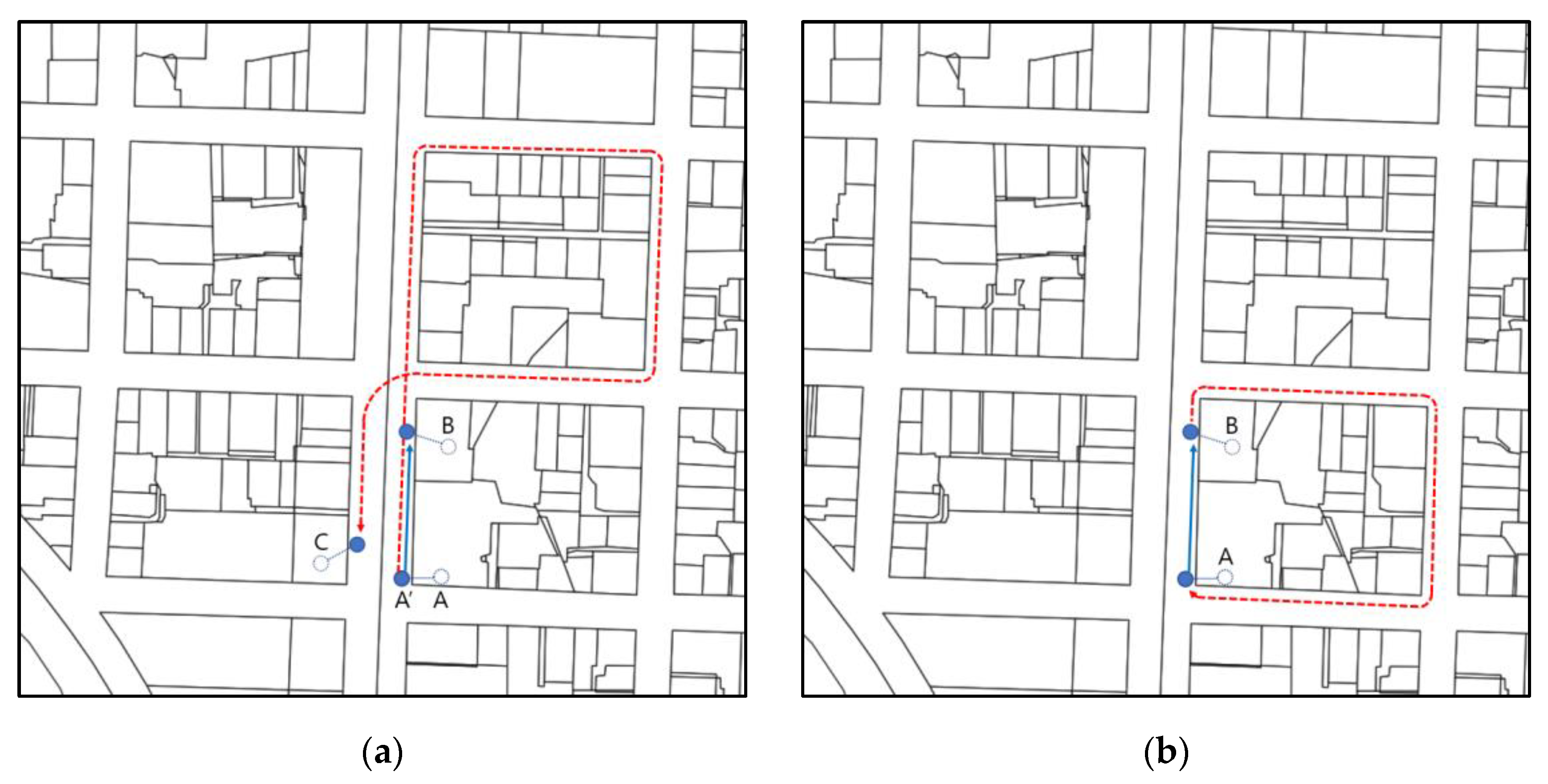
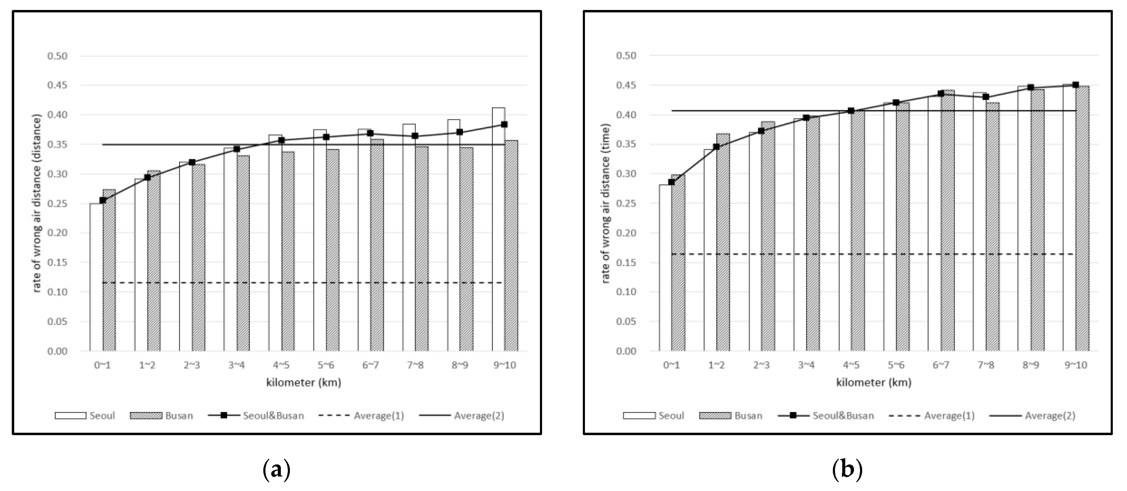
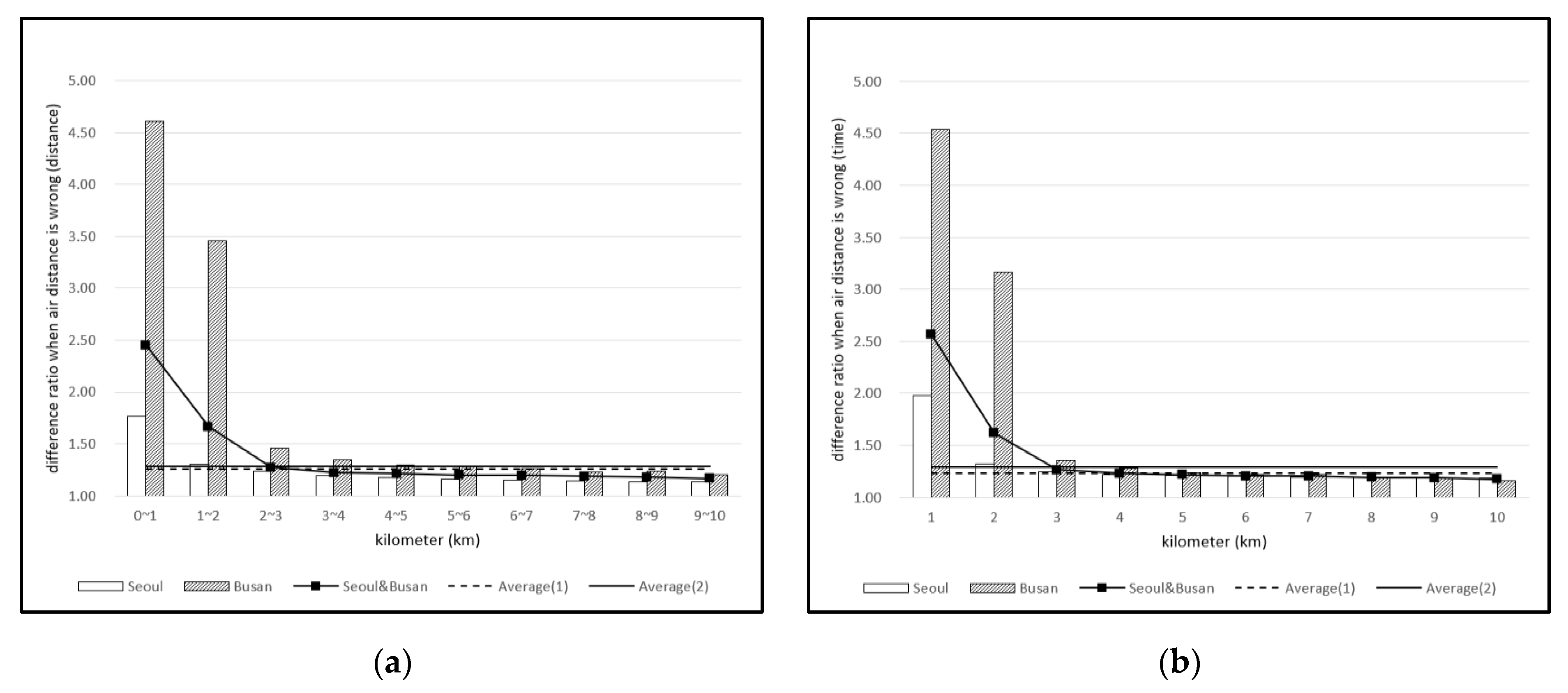
4.1. Closeness Deceived by Air Distance

There is no doubt that air distance can be deceiving when measuring closeness in transportation networks. However, the question of how often and how much has rarely been studied.

Figure 8 and Figure 9 highlight the frequency and magnitude, respectively. More specifically, Figure 8 presents the rate at which the use of air distances and road distances produce different results. Suppose there are three nodes, A, B, and C. The air distances from A to B and from A to C are measured and compared. This same comparison is subsequently carried out using road distance or road time. If the comparison using air distance versus road distance or road time creates different winners, it is assumed that the air distances are inaccurate. Ten distance range boundaries are set for the analyses. The boundaries are based on air distances. For a boundary of {0~1}, the air distances from A to B and from A to C are both within 1 km. Two different average values are displayed in the figure. In a nutshell, average (1) is calculated with nodes with similar air distances, while average (2) also includes cases with dissimilar air distances. The average (1) refers to the average value from all boundaries {0~1, 1~2, …, 9~10}. On the other hand, average (2) is the average value from a different boundary, which is {0~10}. It is natural that average (2) has a lower rate than average (1), since average (2) includes cases where differences in the air distance from A to B and from A to C are within 10 km, while average (1) only includes cases where the differences are within 1 km.

As shown in Figure 8, within the boundaries of 1 km, there is a 34.9% chance that the air distance is wrong for the distance measurement, and a 40.6% chance that it is wrong for the time measurement. Even if the boundary is set to be within 10 km, there still exists a high chance that the air distance will be wrong: 11.6% for distance and 16.4% for time.

In Figure 8, it is noted that using air distance in a time measurement is more likely to be inaccurate than for a distance measurement. This is true because the criterion used is the air distance rather than the air time. It is also noted that as the distance range increases, the rate at which air distance produces inaccurate results also increases.

However, as illustrated in Figure 9, the magnitude of inaccuracy decreases when the distance range increases. For example, in a short distance rage of {0~1} km, the average difference is as high as 2.5 times. That is, if the air distance measurement from A to B is smaller than from A to C, there is about a 25% chance the measurement will be wrong, as shown in Figure 8a. In addition, the road distance measurement (with respect to cost) from A to B will, in fact, be larger than from A to C by 2.5 times. As provided in Figure 9, within the range {0~10}, the average differences are calculated as 27.9% for road distance and 29% for road time.

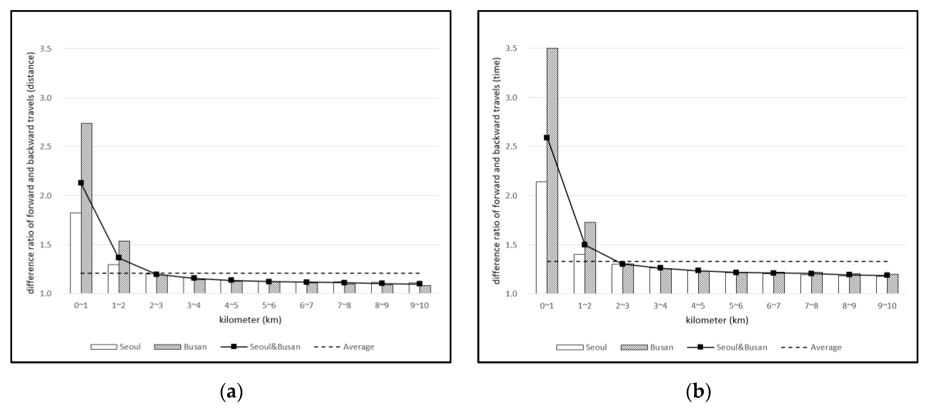
4.2. Assymetric Costs

Another interesting challenge is to determine the differences in costs between the outbound and return trips. The cost differences of the outbound trip from A to B and the return trip from B to A are measured. The difference ratio is calculated, dividing the larger cost by the smaller cost. The results are provided in Figure 10.

As expected, the difference ratio decreases when the distance range increases. In the shortest range where the distance range is only within 1 km, the average difference ratio can be as high as 2.13 times for road distance and 2.59 times for road time. Within the range of {0~10}, there exists a 20.6% difference in distance and a 32.9% difference in time, on average. The difference ratio in road time is computed to be larger than road distance across all boundaries, cities, and averages.

Figure 9 and Figure 10 illuminate the point that different cities, or different areas in a city, can have different road network characteristics. In the analyses, Busan tends to produce higher difference rates than Seoul, especially within smaller boundaries. As can be seen in Figure 5 and Figure 6, Busan is covered with more forested areas, fields and farmlands than Seoul. In addition, the difference in the number of one-way streets can be a factor.

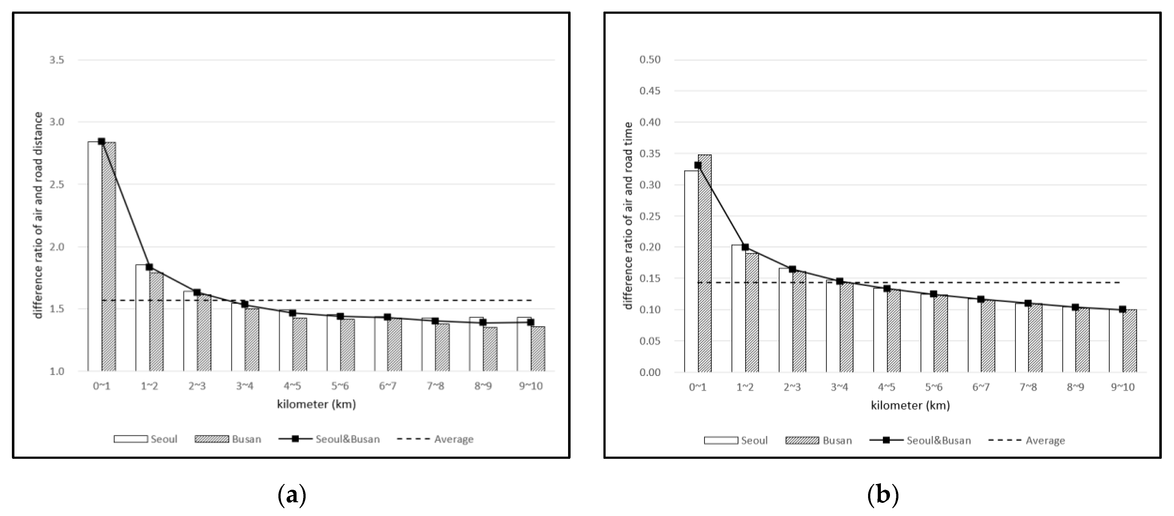
4.3. Air Distance to Road Distance and Road Time Multiplier

Although imprecise, a simple but rough multiplier for transforming air distances into a road distances or road times can be useful. For instance, when solving a vehicle routing problem, the cost of traveling between nodes that are very far apart from each other does not have to be exact. Many of the exceedingly long links are rarely considered or highlighted in problem-solving processes. When employing map APIs, precisely acquiring every single road distance or road time can be costly. It can be costly not only in terms of purchasing costs, but also response times. For this reason, it is attractive to estimate road distances or road times using rough multipliers for those links that exceed a pre-set threshold.

For the general conversion ratio, Figure 11 can provide some guidelines. It is noted that the y-axis in Figure 11a ranges from 1.0 to 3.0. In Figure 11b, it ranges from 0.0 to 0.5. This is because Figure 11a indicates meter-to-meter conversion ratios, while Figure 11b indicates meter-to-second conversion ratios. Road distances are always larger than, or sometimes equal to, the air distances, which causes the ratio to exceed 1.0. However, distance and time are in different scales, and a meter-to-second conversion ratio should only be larger than zero. The conversion ratio decreases with increasing distance ranges. The differences derive from the road network structure, as well as from the speed of the vehicle. In general, average vehicle speed in a long haul is faster than a short one. Arterial roads, trunk lines or expressways are more likely to be used in a long haul. Within 10 km of air distance, the average rough multipliers for road distance and road time are calculated as 1.57 and 0.14, respectively.

5. Discussion

As explained in Section 3.2.3 and Section 4.2, different areas can have different characteristics with respect to road networks. Some areas are covered with more forested areas, fields and farmlands than others. In addition, some areas can include a greater number of one-way streets than others. The proposed benchmark sets and the corresponding analyses may not represent the entire picture and characteristics of a country, or even a city. Although they only provide partial images, the fact that the benchmark instances are realistic remains unchanged.

The analyses in Section 4 are constrained to the maximum distance range of 10 km. This is because when creating road distance and road time matrices, the cost of links that exceed 10 km in terms of air distance are estimated rather than precisely defined, as noted in Section 4.3 using the values of boundary {9~10} in Figure 11. Asymmetry is applied to the estimated road distance and road time using the ratio values of boundary {9~10} provided in Figure 10. We believe this is applicable since we are focused on creating benchmark instances for last-mile deliveries and the distribution of goods in urban settings. Additionally, since 72.6% of the four million pairs are within 10 km of air distance, and 27.4% are not, we are able to conclude that using the majority to assume the remainder is reasonable. More detailed information on the number of cases and the ratios for pairs of nodes within individual air distance ranges are provided in Figure 12.

Road distances and road times between nodes change over the time of day and over the day of the week. This is because the distance or time from the map APIs are based on the shortest or fastest path between nodes, and the greedy paths in the road network change over periods. This is also because there are peak hours and off-peak hours in urban transportation environments. Road distance and road time matrix creation is based on a random time of day to ensure that we accommodate both peak and off-peak hour characteristics in the new benchmark instances and in the analysis.

Even with the limitations discussed above, the newly proposed benchmark instances have merit for a number of reasons. The previously available Fischetti [18], De Smet [22] and Rodríguez [20] instances are all based on European regions. The new instances are the first to be based on an Asian country. In addition, for the purpose of testing cutting-edge VRP solving algorithms on single or multi-objective real-life problems, the new instances are the first to satisfy multiple important qualities simultaneously. Specifically, there are sufficient numbers and dimensions of problem instances, real data are used in the generation of depot and customer node locations, both road time and road distance matrices are present, and best-known solutions (BKS) are available. With these qualities in mind, a comprehensive comparison of the existing and new benchmark instances is provided in

Table 4. Comparison of ACVRP benchmark instances.

Benchmark	Number	Dimensions	Depot and Customer Nodes	Road Distance	Road Time	Reported BKS ***
Fischetti	32 *	34~74	Real data of pharmaceutical product delivery	O	X	O
De Smet	10 **	50~2750	Administrative districts	O	O	X
Rodríguez	2700	50~500	Random, grid, and radial	O	X	X
Proposed instances	648	50~500	Real data of UDCs, postal hubs, large malls, residential complexes, restaurants, and convenience stores	O	O	O

* The original number was eight, but the instances grew in terms of population by modifying vehicle capacity. ** The number of instances is 50, but after netting only the ACVRP instances, 10 instances are available. *** The availability of best-known solutions.

below.

6. Conclusions

Recognizing the lack of benchmark instances in VRPs with asymmetric costs, or ACVRPs, this paper supplemented the instances with new and more realistic ones. The instances were generated with the help of a wide range of publicly shared data and advanced map API services in Korea. They were created using publicly shared spatial data for depot and customer locations. The locations included UDCs, regional hubs for postal services, shopping malls, restaurant businesses, residential facilities, and convenience stores. For road distance and road time matrices, T map, a map API renowned for its accuracy in Korea, was used. A total of 648 ACVRP benchmark instances are now available online.

The proposed benchmark instances contribute to the research community since they carefully and realistically reflect urban transportation environments. Real road distance and road time matrices are asymmetric, and this asymmetry has a large effect over the solution methods and quality in a VRP [4]. The benchmark instances will be useful in the development of routing algorithms. In addition, the proposed instances are based on cities in Korea, which makes them the first benchmarks based on any region outside of Europe. Additionally, this paper is the first to present instances that satisfy all of the following criteria: be large in number, include instances of large dimension, include both road time and road distance matrices, reflect the realities of urban transportation, and provide records on best-known solutions.

Using the benchmark instances’ abundant road distance and road time matrices, this paper analyzed and answered three important questions in urban transportation planning that have rarely been considered: (i) the frequency and magnitude in which air distance differs from reality when measuring closeness, (ii) the differences in distance and time for outgoing and return trips, and (iii) rough conversion ratios from air distance to road distance and road time. The analyses were carried out for each boundary of 1 km within 10 km of air distance.

Overall, using air distance results in inaccurate decisions when measuring closeness. For distance measurements, it is wrong 34.9% of the time by a magnitude of 27.9%. For time measurements, it is wrong 40.6% of the time by 29%. On average, the outbound and return trips differ by 20.6% in distance and 32.9% in time. The value 1.57 may be multiplied to air distance when estimating road distance, and 0.14 may be used when converting air distance in meters into road time in seconds.

The analyses contribute to the research community by highlighting characteristics of urban transportation environments. Furthermore, this paper can be referenced when emphasizing the necessity of using map APIs instead of air distances in transportation planning. This paper provides some managerial implications. Accurate planning can only be conducted with accurate distance and time measurements. It is important to have reliable sources for road distance and road time estimations, particularly in the distribution of goods or in last mile deliveries. Additionally, when distances increase, the inaccuracies incurred by relying on air distances decrease in magnitude, as do the cost differences between the outbound and return trips. For distant node pairs, it is plausible to use rough estimations using the suggested conversion ratio in this paper.

Future research can be directed to overcome some of the limitations discussed in Section 5. The maximum distance range for the analyses in this research was 10 km. Beyond this perimeter, further distances can be explored and analyzed in future research. Moreover, since road distances and road times between nodes can change across the day, peak and off-peak hours can be separated to discover their differences in a future analysis. Finally, and most importantly, ACVRP solving algorithms should be tested using the new benchmark instances. The experiments should focus on the differences in the following two solutions and objective function values (OFVs). The first solution is obtained by using a symmetric air distance matrix, and then corresponding asymmetric road distances or time-matrices are applied to the solution to calculate the total cost. For the second solution, asymmetric road distances or road times are used in the first place. The two solutions can be compared for analysis.

References

1. Eksioglu, B.; Vural, A.V.; Reisman, A. The vehicle routing problem: A taxonomic review. Comput. Ind. Eng. 2009, 57, 1472–1483. [Google Scholar] [CrossRef]
2. Braekers, K.; Ramaekers, K.; Van Nieuwenhuyse, I. The vehicle routing problem: State of the art classification and review. Comput. Ind. Eng. 2016, 99, 300–313. [Google Scholar] [CrossRef]
3. Smet, G. De OptaPlanner—Vehicle Routing with Real Road Distances. Available online: https://www.optaplanner.org/blog/2014/09/02/VehicleRoutingWithRealRoadDistances.html (accessed on 28 December 2020).
4. Rodríguez, A.; Ruiz, R. A study on the effect of the asymmetry on real capacitated vehicle routing problems. Comput. Oper. Res. 2012, 39, 2142–2151. [Google Scholar] [CrossRef] [Green Version]
5. Cho, H.J.; Park, C. The leadership competition of smart platforms in the ICT ecosystem: Comparative analysis of samsung electronics and SK telecom in the appcessory market. Asia Pac. J. Bus. Ventur. Entrep. 2015, 10, 187–202. [Google Scholar]
6. Lee, H.; Park, H.C.; Kho, S.Y.; Kim, D.K. Assessing transit competitiveness in Seoul considering actual transit travel times based on smart card data. J. Transp. Geogr. 2019, 80, 102546. [Google Scholar] [CrossRef]
7. Caceres-Cruz, J.; Arias, P.; Guimarans, D.; Riera, D.; Juan, A.A. Rich vehicle routing problem: Survey. ACM Comput. Surv. 2014, 47. [Google Scholar] [CrossRef]
8. Rodríguez, A.; Ruiz, R. The effect of the asymmetry of road transportation networks on the traveling salesman problem. Comput. Oper. Res. 2012, 39, 1566–1576. [Google Scholar] [CrossRef] [Green Version]
9. Cáceres-Cruz, J.; Riera, D.; Buil, R.; Juan, A.A.; Herrero, R. Multi-start approach for solving an asymmetric heterogeneous vehicle routing problem in a real urban context. In Proceedings of the 2nd International Conference on Operations Research and Enterprise Systems (ICORES-2013), Barcelona, Spain, 16–18 February 2013; pp. 168–174. [Google Scholar] [CrossRef]
10. Herrero, R.; Rodríguez, A.; Cáceres-Cruz, J.; Juan, A.A. Solving vehicle routing problems with asymmetric costs and heterogeneous fleets. Int. J. Adv. Oper. Manag. 2015, 6, 58–80. [Google Scholar] [CrossRef] [Green Version]
11. Laporte, G.; Mercure, H.; Nobert, Y. An exact algorithm for the asymmetrical capacitated vehicle routing problem. Networks 1986, 16, 33–46. [Google Scholar] [CrossRef]
12. Laporte, G.; Nobert, Y.; Taillefer, S. A branch-and-bound algorithm for the asymmetrical distance-constrained vehicle routing problem. Math. Model. 1987, 9, 857–868. [Google Scholar] [CrossRef] [Green Version]
13. Toth, P.; Vigo, D. A heuristic algorithm for the symmetric and asymmetric vehicle routing problems with backhauls. Eur. J. Oper. Res. 1999, 113, 528–543. [Google Scholar] [CrossRef]
14. Osaba, E.; Yang, X.S.; Diaz, F.; Onieva, E.; Masegosa, A.D.; Perallos, A. A discrete firefly algorithm to solve a rich vehicle routing problem modelling a newspaper distribution system with recycling policy. Soft Comput. 2017, 21, 5295–5308. [Google Scholar] [CrossRef] [Green Version]
15. Lee, K.; Chae, J.; Song, B.; Choi, D. A model for sustainable courier services: Vehicle routing with exclusive lanes. Sustainability 2020, 12, 1077. [Google Scholar] [CrossRef] [Green Version]
16. Calvet, L.; Pagès-Bernaus, A.; Travesset-Baro, O.; Juan, A.A. A simheuristic for the heterogeneous site-dependent asymmetric VRP with stochastic demands. In Lecture Notes Computer Science; Spring: Cham, Switzerland, 2016; Volume 9868, pp. 408–417. [Google Scholar] [CrossRef]
17. Ilin, V.; Matijević, L.; Davidović, T.; Pardalos, P. Asymmetric Capacitated Vehicle Routing Problem with Time Window. In Proceedings of the XLV Symposium on Operational Research (SYM-OP-IS 2018), Zlatibor, Serbia, 16–18 September 2018; pp. 174–179. Available online: http://researchrepository.mi.sanu.ac.rs/handle/123456789/3174 (accessed on 22 May 2021).
18. Fischetti, M.; Toth, P.; Vigo, D. A branch-and-bound algorithm for the capacitated vehicle routing problem on directed graphs. Oper. Res. 1994, 42, 846–859. [Google Scholar] [CrossRef]
19. Pessoa, A.; de Aragao, M.P.; Uchoa, E. Robust Branch-Cut-and-Price Algorithms for Vehicle Routing Problems; Springer: Boston, MA, USA, 2008; Volume 43, ISBN 9780387777788. [Google Scholar]
20. Rodríguez, A.; Ruiz, R. ACVRP_Depot Problem Instances. Available online: http://soa.iti.es/problem-instances (accessed on 28 December 2020).
21. Distance Matrix API. Available online: https://developers.google.com/maps/documentation/distance-matrix/overview (accessed on 11 March 2021).
22. Smet, G. De VRP-REP_the Vehicle Routing Problem Repository. Available online: http://www.vrp-rep.org/datasets/item/2017-0001.html (accessed on 6 January 2021).
23. Routing—OpenStreetMap. Available online: https://wiki.openstreetmap.org/wiki/Routing (accessed on 24 March 2021).
24. Li, R.; Cheng, C.; Qi, M.; Lai, W. Design of dynamic vehicle routing system based on online map service. In Proceedings of the 2016 13th International Conference on Service Systems and Service Management (ICSSSM), Kunming, China, 24–26 June 2016; pp. 1–5. [Google Scholar] [CrossRef]
25. Hashi, E.K.; Hasan, M.R.; Zaman, M.S.U. GIS based heuristic solution of the vehicle routing problem to optimize the school bus routing and scheduling. In Proceedings of the 2016 19th International Conference on Computer and Information Technology (ICCIT), Dhaka, Bangladesh, 18–20 December 2016; pp. 56–60. [Google Scholar] [CrossRef]
26. Welch, P. Developing a commercial dynamic vehicle routing system—a case study. Open Door Logist. 2017. [Google Scholar] [CrossRef]
27. Baidu Map Data Open Platform. Available online: http://lbsyun.baidu.com (accessed on 24 March 2021).
28. Li, Y.; Lim, M.K.; Tseng, M.L. A green vehicle routing model based on modified particle swarm optimization for cold chain logistics. Ind. Manag. Data Syst. 2019, 119, 473–494. [Google Scholar] [CrossRef]
29. Wang, Y.; Assogba, K.; Fan, J.; Xu, M.; Liu, Y.; Wang, H. Multi-Depot green vehicle routing problem with shared transportation resource: Integration of time-dependent speed and piecewise penalty cost. J. Clean. Prod. 2019, 232, 12–29. [Google Scholar] [CrossRef]
30. Qi, C.; Hu, L. Optimization of vehicle routing problem for emergency cold chain logistics based on minimum loss. Phys. Commun. 2020, 40, 101085. [Google Scholar] [CrossRef]
31. Lee, K.; Chae, J.; Kim, J. A courier service with electric bicycles in an Urban Area: The case in Seoul. Sustainability 2019, 11, 1255. [Google Scholar] [CrossRef] [Green Version]
32. Lee, K.; Chae, J.; Cha, H.; Song, J. Mendeley Data—New Realistic Sets of Benchmark Instances for Vehicle Routing Problem with Asymmetric Costs. Available online: http://dx.doi.org/10.17632/5db8mtw4wg.2 (accessed on 22 May 2021).
33. Seoul Districts. Available online: https://en.wikipedia.org/wiki/File:Map_Seoul_districts_de.png (accessed on 28 March 2021).
34. Busan Districts. Available online: https://en.wikipedia.org/wiki/Busan (accessed on 28 March 2021).
35. Average Load Factor by Freight Vehicle Capacity. Available online: https://kosis.kr/statHtml/statHtml.do?orgId=116&tblId=DT_MLTM_5414&conn_path=I2 (accessed on 30 March 2021).
36. Diana, M.; Pirra, M.; Woodcock, A. Freight distribution in urban areas: A method to select the most important loading and unloading areas and a survey tool to investigate related demand patterns. Eur. Transp. Res. Rev. 2020, 12. [Google Scholar] [CrossRef]
37. Gillett, B.E.; Miller, L.R. A Heuristic Algorithm for the Vehicle-Dispatch Problem. Oper. Res. 1974, 22, 340–349. [Google Scholar] [CrossRef]
38. Kirkpatrick, S.; Gelatt, C.D.; Vecchi, M.P. Optimization by simulated annealing. Science 1983, 220, 671–680. [Google Scholar] [CrossRef] [PubMed]
Figure 1. A figurative explanation on using map APIs: (a) The air distance underrepresents the actual travel distance; (b) the outbound and return trip costs are different.
Applsci 11 04790 g001
Figure 2. Examples of locations in random (left), grid (middle) and radial (right) distributions [8].
Applsci 11 04790 g002
Figure 3. Map of Seoul, Korea: (a) Administrative districts [33]; (b) vector image on a GIS application.
Applsci 11 04790 g003
Figure 4. Map of Busan, Korea: (a) Administrative districts [34]; (b) vector image on a GIS application.
Applsci 11 04790 g004
Figure 5. An area in Seoul marked with entities of interest (red circles: restaurant businesses; green diamonds: residential complexes; yellow triangles: convenience stores; blue squares: large shopping malls).
Applsci 11 04790 g005
Figure 6. An area in Busan marked with entities of interest (red circles: restaurant businesses; green diamonds: residential complexes; yellow triangles: convenience stores; blue squares: large shopping malls).
Applsci 11 04790 g006
Figure 7. Distribution of delivery weight and volume for an order: (a) Delivery weight; (b) delivery volume.
Applsci 11 04790 g007
Figure 8. The ratio of closeness deceived by air distance: (a) Road distance; (b) road time.
Applsci 11 04790 g008
Figure 9. The magnitude of closeness deceived by air distance: (a) Road distance; (b) road time.
Applsci 11 04790 g009
Figure 10. Cost difference between outbound and return trips: (a) Road distance; (b) road time.
Applsci 11 04790 g010
Figure 11. General conversion ratio for air distance: (a) to road distance; (b) to road time.
Applsci 11 04790 g011
Figure 12. The number and ratio for node pairs regarding air distance.
Applsci 11 04790 g012