
Design of a Multimodal Imaging System and Its First Application to Distinguish Grey and White Matter of Brain Tissue. A Proof-of-Concept-Study

 , , , and
Abstract
1. Introduction
2. Materials and Methods
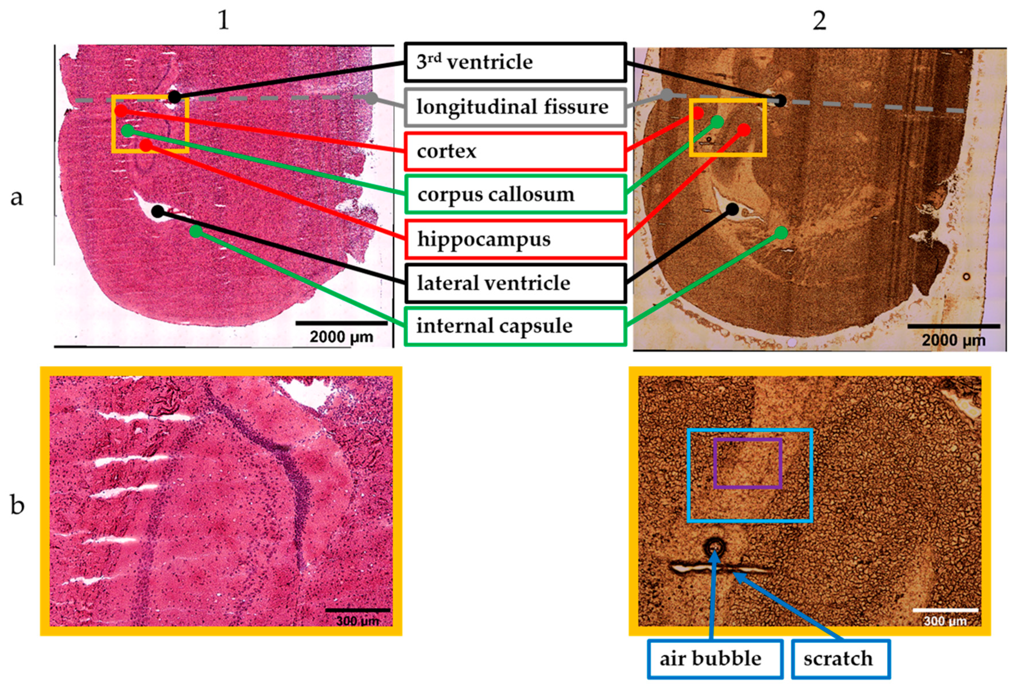
2.1. Sample Preparation
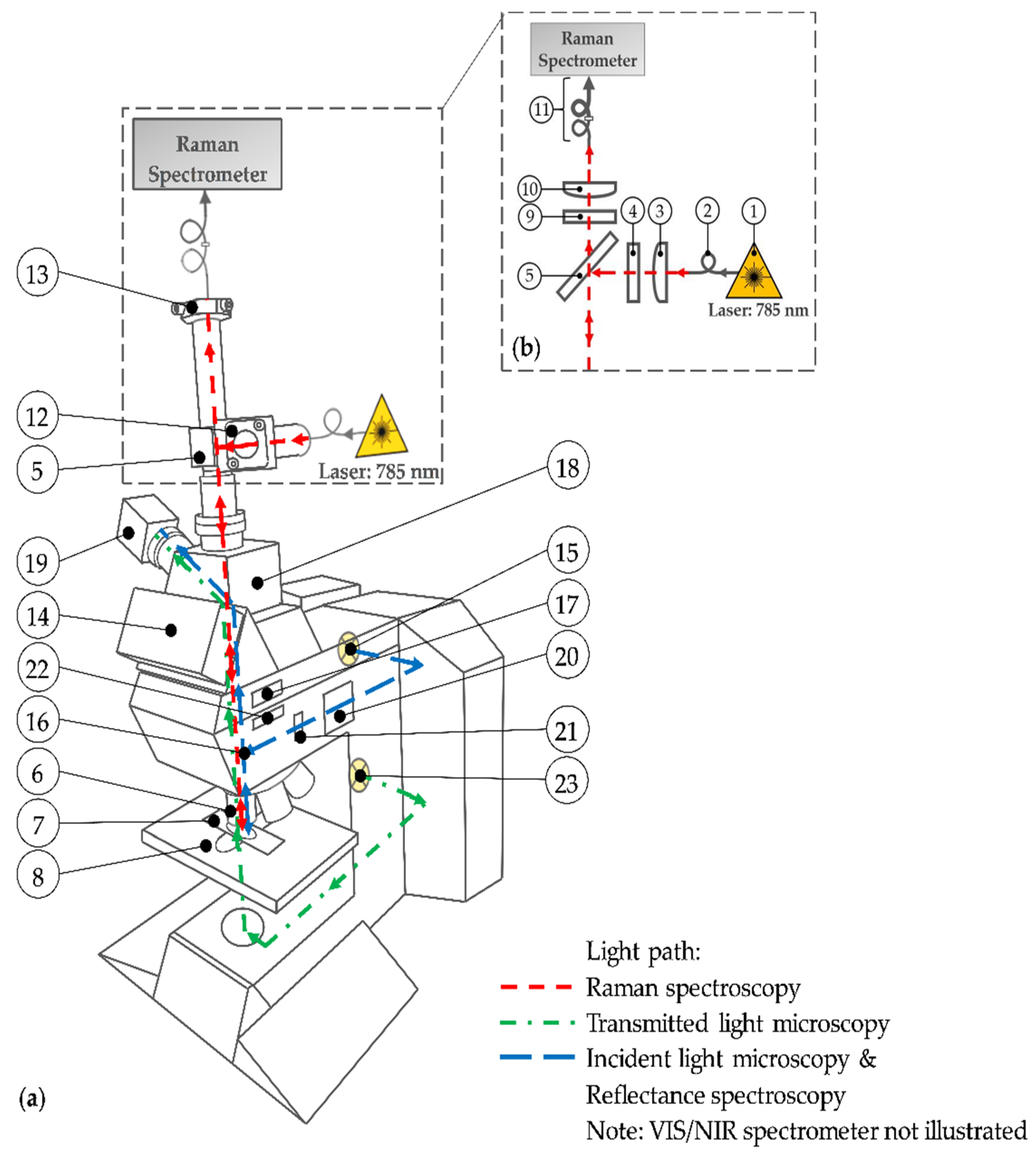
2.2. Multimodal Imaging System
2.3. Data Acquisition
2.4. Image Creation and Spectra Processing
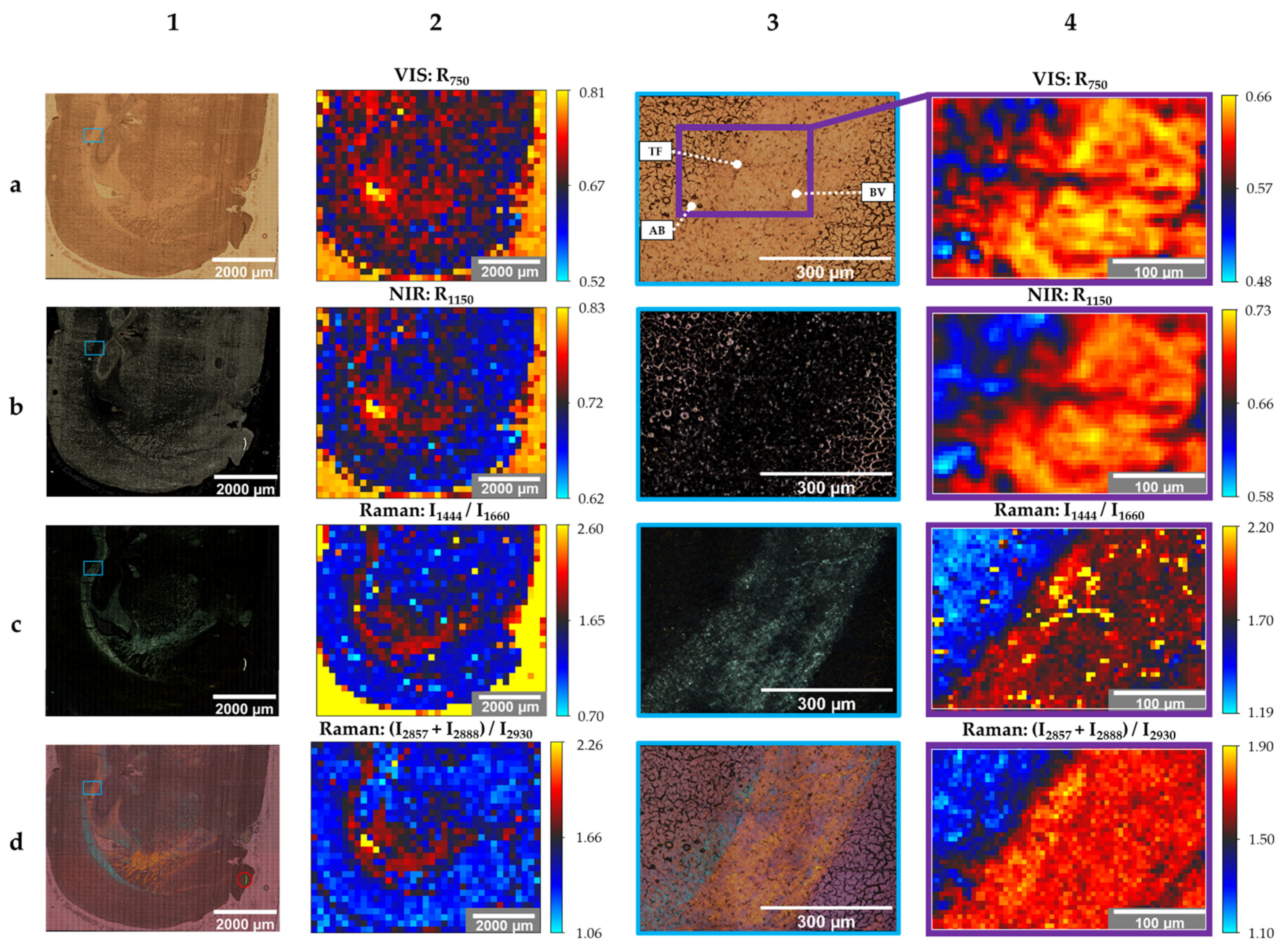
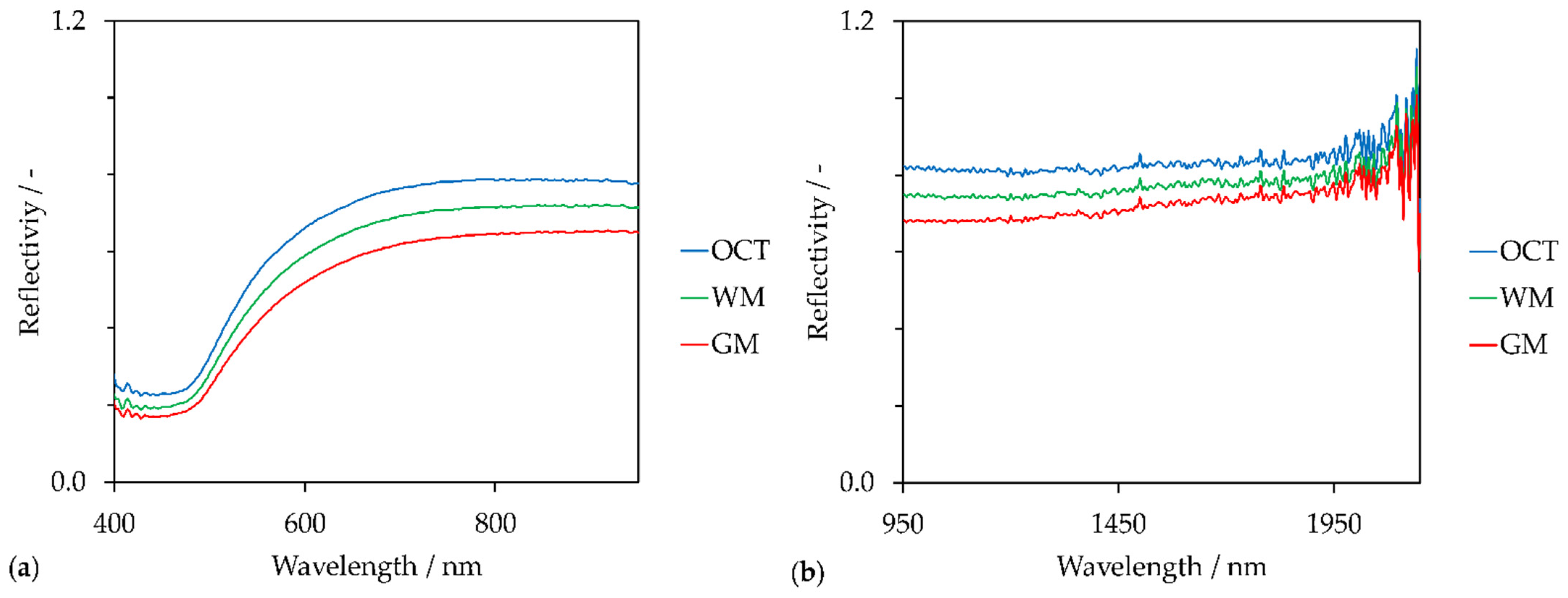
3. Results
4. Discussion
5. Conclusions
Author Contributions
Funding
Institutional Review Board Statement
Informed Consent Statement
Conflicts of Interest
Appendix A


References
- Paramitha, D.; Ulum, M.; Purnama, A.; Wicaksono, D.; Noviana, D.; Hermawan, H. Monitoring degradation products and metal ions in vivo. In Monitoring and Evaluation of Biomaterials and their Performance In Vivo; Narayan, R., Ed.; Elsevier: Amsterdam, The Netherlands, 2017; pp. 19–38. [Google Scholar]
- Krafft, C.; Jürgen, P. Vibrational Spectroscopic Imaging of Soft Tissue. In Infrared and Raman Spectroscopic Imaging; 2nd Completely Revised and Updated Edition; Salzer, R., Siesler, H.W., Eds.; Wiley-VCH: Weinheim, Germany, 2014; pp. 113–152. ISBN 978-3-527-33652-4. [Google Scholar]
- Mireskandari, M.; Petersen, I. Clinical Pathology. In Ex-vivo and In-vivo Optical Molecular Pathology; Popp, J., Ed.; Wiley: Weinheim, Germany, 2014; pp. 1–26. ISBN 978-3-527-33513-8. [Google Scholar]
- Vogler, N.; Heuke, S.; Bocklitz, T.W.; Schmitt, M.; Popp, J. Multimodal Imaging Spectroscopy of Tissue. Annu. Rev. Anal. Chem. (Palo Alto California) 2015, 8, 359–387. [Google Scholar] [CrossRef]
- Schäfer, L. Histologische Techniken. In Histopathologie der Haut; Cerroni, L., Garbe, C., Metze, D., Kutzner, H., Kerl, H., Eds.; Springer: Berlin/Heidelberg, Germany, 2016; pp. 3–13. ISBN 978-3-662-45132-8. [Google Scholar]
- Baumann, B. Optical Coherence Tomotgraphy for Brain Imaging. In Advanced Optical Methods for Brain Imaging; Kao, F.-J., Keiser, G., Gogoi, A., Eds.; Springer: Singapore, 2019; pp. 49–68. ISBN 978-981-10-9019-6. [Google Scholar]
- Pfister, M.; Schützenberger, K.; Schäfer, B.J.; Puchner, S.; Stegmann, H.; Hohenadl, C.; Mildner, M.; Garhöfer, G.; Schmetterer, L.; Werkmeister, R.M. Optical Coherence Tomography Angiography Monitors Cutaneous Wound Healing under Angio-genesis-Promoting Treatment in Diabetic and Non-Diabetic Mice. Appl. Sci. 2021, 11, 2447. [Google Scholar] [CrossRef]
- Liu, G.; Chen, Z. Optical Coherence Tomography for Brain Imaging. In Optical Methods and Instrumentation in Brain Imaging and Therapy; Madsen, S.J., Ed.; Springer: New York, NY, USA, 2013; pp. 157–172. ISBN 978-1-4614-4977-5. [Google Scholar]
- Zysk, A.M.; Boppart, S.A. Optical Coherence Tomography. In Optical Imaging and Microscopy: Techniques and Advanced Systems; 2nd Revised Edition; Török, P., Kao, F.-J., Eds.; Springer: Berlin, Germany, 2007; pp. 401–436. ISBN 978-3-540-69563-9. [Google Scholar]
- Guthoff, R.F.; Baudouin, C.; Stave, J. Atlas of Confocal Laser Scanning In-Vivo Microscopy in Ophthalmology: Principles and Applications in Diagnostic and Therapeutic Ophthalmology; Springer: Berlin, Germany, 2006; ISBN 978-3-540-32705-9. [Google Scholar]
- Hofmann-Wellenhof, R.; Pellacani, G.; Malvehy, J.; Soyer, H.P. Reflectance Confocal Microscopy for Skin Diseases; Springer: Berlin, Germany, 2012; ISBN 978-3-642-21996-2. [Google Scholar]
- Bağcı, I.S.; Aoki, R.; Krammer, S.; Ruzicka, T.; Sárdy, M.; Hartmann, D. Ex vivo confocal laser scanning microscopy: An in-novative method for direct immunofluorescence of cutaneous vasculitis. J. Biophotonics 2019, 12, e201800425. [Google Scholar] [CrossRef] [PubMed]
- Yildirim, M.; Quinn, K.P.; Kobler, J.B.; Zeitels, S.M.; Georgakoudi, I.; Ben-Yakar, A. Quantitative differentiation of normal and scarred tissues using second-harmonic generation microscopy. Scanning 2016, 38, 684–693. [Google Scholar] [CrossRef] [PubMed]
- Tan, H.-Y.; Chang, Y.-L.; Lo, W.; Hsueh, C.-M.; Chen, W.-L.; Ghazaryan, A.A.; Hu, P.-S.; Young, T.-H.; Chen, S.-J.; Dong, C.-Y. Characterizing the morphologic changes in collagen crosslinked-treated corneas by Fourier transform-second harmonic generation imaging. J. Cataract Refract. Surg. 2013, 39, 779–788. [Google Scholar] [CrossRef]
- Kawakami, R.; Nemoto, T. In Vivo Imaging of All Cortical Layers and Hippocampal CA1 Pyramidal Cells by Two-Photon Excitation Microscopy. In Advanced Optical Methods for Brain Imaging; Kao, F.-J., Keiser, G., Gogoi, A., Eds.; Springer: Singapore, 2019; pp. 113–122. ISBN 978-981-10-9019-6. [Google Scholar]
- Piston, D.W. Two-Photon Excitation Microscopy for Three-Dimensional Imaging of Living Intact Tissues. In Fluorescence Microscopy: From Principles to Biological Applications, Second Edition; Kubitscheck, U., Ed.; Wiley-VCH: Weinheim, Germany, 2017; pp. 203–242. ISBN 978-3-527-33837-5. [Google Scholar]
- Delhaye, M.; Dhamelincourt, P. Raman microprobe and microscope with laser excitation. J. Raman Spectrosc. 1975, 3, 33–43. [Google Scholar] [CrossRef]
- Hollricher, O. Raman Instrumentation for Confocal Raman Microscopy. In Confocal Raman Microscopy; Dieing, T., Ed.; Springer: Berlin, Germany, 2010; pp. 43–60. ISBN 978-3-642-12522-5. [Google Scholar]
- Smekal, A. Zur Quantentheorie der Dispersion. Naturwissenschaften 1923, 11, 873–875. [Google Scholar] [CrossRef]
- Raman, C.V.; Krishnan, K.S. A New Type of Secondary Radiation. Nature 1928, 121, 501–502. [Google Scholar] [CrossRef]
- Butler, H.J.; Ashton, L.; Bird, B.; Cinque, G.; Curtis, K.; Dorney, J.; Esmonde-White, K.; Fullwood, N.J.; Gardner, B.; Martin-Hirsch, P.L.; et al. Using Raman spectroscopy to characterize biological materials. Nat. Protoc. 2016, 11, 664–687. [Google Scholar] [CrossRef]
- Petry, R.; Schmitt, M.; Popp, J. Raman spectroscopy--a prospective tool in the life sciences. Chemphyschem 2003, 4, 14–30. [Google Scholar] [CrossRef]
- Kiselev, R.; Schie, I.W.; Aškrabić, S.; Krafft, C.; Popp, J. Design and first applications of a flexible Raman micro-spectroscopic system for biological imaging. BSI 2016, 5, 115–127. [Google Scholar] [CrossRef]
- Vandenabeele, P. Practical Raman Spectroscopy: An Introduction; Wiley: Chichester, UK, 2013; ISBN 978-0-470-68319-4. [Google Scholar]
- Schalk, R.; Heintz, A.; Braun, F.; Iacono, G.; Rädle, M.; Gretz, N.; Methner, F.-J.; Beuermann, T. Comparison of Raman and Mid-Infrared Spectroscopy for Real-Time Monitoring of Yeast Fermentations: A Proof-of-Concept for Multi-Channel Photometric Sensors. Appl. Sci. 2019, 9, 2472. [Google Scholar] [CrossRef]
- Hollricher, O.; Ibach, W. High-Resolution Optical and Confocal Microscopy. In Confocal Raman Microscopy; Dieing, T., Ed.; Springer: Berlin, Germany, 2010; pp. 1–20. ISBN 978-3-642-12522-5. [Google Scholar]
- Tuschel, D. Selecting an Excitation Wavelength for Raman Spectroscopy. Spectroscopy 2016, 31, 14–23. [Google Scholar]
- Cui, L.; Butler, H.J.; Martin-Hirsch, P.L.; Martin, F.L. Aluminium foil as a potential substrate for ATR-FTIR, transflection FTIR or Raman spectrochemical analysis of biological specimens. Anal. Methods 2016, 8, 481–487. [Google Scholar] [CrossRef]
- Fullwood, L.M.; Griffiths, D.; Ashton, K.; Dawson, T.; Lea, R.W.; Davis, C.; Bonnier, F.; Byrne, H.J.; Baker, M.J. Effect of sub-strate choice and tissue type on tissue preparation for spectral histopathology by Raman microspectroscopy. Analyst 2014, 139, 446–454. [Google Scholar] [CrossRef]
- Jones, R.R.; Hooper, D.C.; Zhang, L.; Wolverson, D.; Valev, V.K. Raman Techniques: Fundamentals and Frontiers. Nanoscale Res. Lett. 2019, 14, 231. [Google Scholar] [CrossRef] [PubMed]
- Brozek-Pluska, B.; Kopec, M. Raman microspectroscopy of Hematoporphyrins. Imaging of the noncancerous and the cancerous human breast tissues with photosensitizers. Spectrochim. Acta A Mol. Biomol. Spectrosc. 2016, 169, 182–191. [Google Scholar] [CrossRef] [PubMed]
- Abramczyk, H.; Brozek-Pluska, B.; Kopec, M. Polarized Raman microscopy imaging: Capabilities and challenges for cancer research. J. Mol. Liq. 2018, 259, 102–111. [Google Scholar] [CrossRef]
- Mizuno, A.; Hayashi, T.; Tashibu, K.; Maraishi, S.; Kawauchi, K.; Ozaki, Y. Near-infrared FT-Raman spectra of the rat brain tissues. Neurosci. Lett. 1992, 141, 47–52. [Google Scholar] [CrossRef]
- Kast, R.E.; Auner, G.W.; Rosenblum, M.L.; Mikkelsen, T.; Yurgelevic, S.M.; Raghunathan, A.; Poisson, L.M.; Kalkanis, S.N. Raman molecular imaging of brain frozen tissue sections. J. Neurooncol. 2014, 120, 55–62. [Google Scholar] [CrossRef]
- Kast, R.; Auner, G.; Yurgelevic, S.; Broadbent, B.; Raghunathan, A.; Poisson, L.M.; Mikkelsen, T.; Rosenblum, M.L.; Kalkanis, S.N. Identification of regions of normal grey matter and white matter from pathologic glioblastoma and necrosis in frozen sections using Raman imaging. J. Neurooncol. 2015, 125, 287–295. [Google Scholar] [CrossRef]
- Kalkanis, S.N.; Kast, R.E.; Rosenblum, M.L.; Mikkelsen, T.; Yurgelevic, S.M.; Nelson, K.M.; Raghunathan, A.; Poisson, L.M.; Auner, G.W. Raman spectroscopy to distinguish grey matter, necrosis, and glioblastoma multiforme in frozen tissue sections. J. Neurooncol. 2014, 116, 477–485. [Google Scholar] [CrossRef] [PubMed]
- Brozek-Pluska, B.; Musial, J.; Kordek, R.; Abramczyk, H. Analysis of Human Colon by Raman Spectroscopy and Imaging-Elucidation of Biochemical Changes in Carcinogenesis. Int. J. Mol. Sci. 2019, 20, 3398. [Google Scholar] [CrossRef] [PubMed]
- Ali, S.M.; Bonnier, F.; Tfayli, A.; Lambkin, H.; Flynn, K.; McDonagh, V.; Healy, C.; Clive Lee, T.; Lyng, F.M.; Byrne, H.J. Raman spectroscopic analysis of human skin tissue sections ex-vivo: Evaluation of the effects of tissue processing and dewaxing. J. Biomed. Opt. 2013, 18, 61202. [Google Scholar] [CrossRef] [PubMed]
- Bonnier, F.; Ali, S.M.; Knief, P.; Lambkin, H.; Flynn, K.; McDonagh, V.; Healy, C.; Lee, T.C.; Lyng, F.M.; Byrne, H.J. Analysis of human skin tissue by Raman microspectroscopy: Dealing with the background. Vib. Spectrosc. 2012, 61, 124–132. [Google Scholar] [CrossRef]
- Bonnier, F.; Mehmood, A.; Knief, P.; Meade, A.D.; Hornebeck, W.; Lambkin, H.; Flynn, K.; McDonagh, V.; Healy, C.; Lee, T.C.; et al. In vitro analysis of immersed human tissues by Raman microspectroscopy. J. Raman Spectrosc. 2011, 42, 888–896. [Google Scholar] [CrossRef]
- Wang, S.; Liang, Z.; Gong, Y.; Yin, Y.; Wang, K.; He, Q.; Wang, Z.; Bai, J. Confocal raman microspectral imaging of ex vivo human spinal cord tissue. J. Photochem. Photobiol. B 2016, 163, 177–184. [Google Scholar] [CrossRef]
- Li, J.; Liang, Z.; Wang, S.; Wang, Z.; Zhang, X.; Hu, X.; Wang, K.; He, Q.; Bai, J. Study on the pathological and biomedical characteristics of spinal cord injury by confocal Raman microspectral imaging. Spectrochim. Acta A Mol. Biomol. Spectrosc. 2019, 210, 148–158. [Google Scholar] [CrossRef]
- Tuck, M.; Blanc, L.; Touti, R.; Patterson, N.H.; van Nuffel, S.; Villette, S.; Taveau, J.-C.; Römpp, A.; Brunelle, A.; Lecomte, S.; et al. Multimodal Imaging Based on Vibrational Spectroscopies and Mass Spectrometry Imaging Applied to Biological Tissue: A Multiscale and Multiomics Review. Anal. Chem. 2021, 93, 445–477. [Google Scholar] [CrossRef]
- De Bettignies, P. Optics/instrumentation. Phys. Sci. Rev. 2020, 5. [Google Scholar] [CrossRef]
- Bashkatov, A.N.; Zakharov, V.P.; Bucharskaya, A.B.; Borisova, E.G.; Khristoforova, Y.A.; Genina, E.A.; Tuchin, V.V. Malignant Tissue Optical Properties. In Multimodal Optical Diagnostics of Cancer; Tuchin, V.V., Popp, J., Zakharov, V., Eds.; Springer International Publishing: Cham, Switzerland, 2020; pp. 3–43. ISBN 978-3-030-44593-5. [Google Scholar]
- Kochan, K.; Chrabaszcz, K.; Szczur, B.; Maslak, E.; Dybas, J.; Marzec, K.M. IR and Raman imaging of murine brains from control and ApoE/LDLR(−/−) mice with advanced atherosclerosis. Analyst 2016, 141, 5329–5338. [Google Scholar] [CrossRef] [PubMed]
- Bunaciu, A.A.; Hoang, V.D.; Aboul-Enein, H.Y. Vibrational Micro-Spectroscopy of Human Tissues Analysis: Review. Crit. Rev. Anal. Chem. 2017, 47, 194–203. [Google Scholar] [CrossRef] [PubMed]
- Lyng, F.; Ramos, I.; Ibrahim, O.; Byrne, H. Vibrational Microspectroscopy for Cancer Screening. Appl. Sci. 2015, 5, 23–35. [Google Scholar] [CrossRef]
- Lasch, P.; Noda, I. Two-Dimensional Correlation Spectroscopy for Multimodal Analysis of FT-IR, Raman, and MALDI-TOF MS Hyperspectral Images with Hamster Brain Tissue. Anal. Chem. 2017, 89, 5008–5016. [Google Scholar] [CrossRef] [PubMed]
- Bovenkamp, D.; Sentosa, R.; Rank, E.; Erkkilä, M.; Placzek, F.; Püls, J.; Drexler, W.; Leitgeb, R.; Garstka, N.; Shariat, S.; et al. Combination of High-Resolution Optical Coherence Tomography and Raman Spectroscopy for Improved Staging and Grading in Bladder Cancer. Appl. Sci. 2018, 8, 2371. [Google Scholar] [CrossRef]
- Egodage, K.; Dochow, S.; Bocklitz, T.; Chernavskaia, O.; Matthaeus, C.; Schmitt, M.; Popp, J. The combination of optical co-herence tomography and Raman spectroscopy for tissue characterization. JBPE 2015, 169–177. [Google Scholar] [CrossRef]
- Bocklitz, T.W.; Salah, F.S.; Vogler, N.; Heuke, S.; Chernavskaia, O.; Schmidt, C.; Waldner, M.J.; Greten, F.R.; Bräuer, R.; Schmitt, M.; et al. Pseudo-HE images derived from CARS/TPEF/SHG multimodal imaging in combination with Raman-spectroscopy as a pathological screening tool. BMC Cancer 2016, 16, 534. [Google Scholar] [CrossRef]
- Das, N.K.; Dai, Y.; Liu, P.; Hu, C.; Tong, L.; Chen, X.; Smith, Z.J. Raman Plus X: Biomedical Applications of Multimodal Raman Spectroscopy. Sensors 2017, 17, 1592. [Google Scholar] [CrossRef]
- Sanchez-Molina, P.; Kreuzer, M.; Benseny-Cases, N.; Valente, T.; Almolda, B.; González, B.; Castellano, B.; Perálvarez-Marín, A. From Mouse to Human: Comparative Analysis between Grey and White Matter by Synchrotron-Fourier Transformed Infrared Microspectroscopy. Biomolecules 2020, 10, 1099. [Google Scholar] [CrossRef]
- Beljebbar, A.; Dukic, S.; Amharref, N.; Manfait, M. Ex vivo and in vivo diagnosis of C6 glioblastoma development by Ra-man spectroscopy coupled to a microprobe. Anal. Bioanal. Chem. 2010, 398, 477–487. [Google Scholar] [CrossRef] [PubMed]
- Ji, M.; Orringer, D.A.; Freudiger, C.W.; Ramkissoon, S.; Liu, X.; Lau, D.; Golby, A.J.; Norton, I.; Hayashi, M.; Agar, N.Y.R.; et al. Rapid, label-free detection of brain tumors with stimulated Raman scattering microscopy. Sci. Transl. Med. 2013, 5, 201ra119. [Google Scholar] [CrossRef]
- Leica Microsystems Wetzlar GmbH. Leica DM R: Instructions; Leica Microsystems: Wetzlar, Germany, 2000. [Google Scholar]
- Zoubir, A. Raman Imaging: Techniques and Applications; Springer: Berlin/Heidelberg, Germany, 2012; ISBN 978-3-642-28251-5. [Google Scholar]
- Preibisch, S.; Saalfeld, S.; Tomancak, P. Globally optimal stitching of tiled 3D microscopic image acquisitions. Bioinformatics 2009, 25, 1463–1465. [Google Scholar] [CrossRef] [PubMed]
- Otto, M. Analytische Chemie; VCH: Weinheim, Germany, 1995; ISBN 9783527286911. [Google Scholar]
- Byrne, H.J.; Knief, P.; Keating, M.E.; Bonnier, F. Spectral pre and post processing for infrared and Raman spectroscopy of biological tissues and cells. Chem. Soc. Rev. 2016, 45, 1865–1878. [Google Scholar] [CrossRef] [PubMed]
- Bocklitz, T.; Walter, A.; Hartmann, K.; Rösch, P.; Popp, J. How to pre-process Raman spectra for reliable and stable models? Anal. Chim. Acta 2011, 704, 47–56. [Google Scholar] [CrossRef] [PubMed]
- Whitaker, D.; Hayes, K. A Simple Algorithm for Despiking Raman Spectra. Chemom. Intell. Lab. Syst. 2018, 179, 82–84. [Google Scholar] [CrossRef]
- He, S.; Zhang, W.; Liu, L.; Huang, Y.; He, J.; Xie, W.; Wu, P.; Du, C. Baseline correction for Raman spectra using an improved asymmetric least squares method. Anal. Methods 2014, 6, 4402–4407. [Google Scholar] [CrossRef]
- Savitzky, A.; Golay, M.J.E. Smoothing and Differentiation of Data by Simplified Least Squares Procedures. Anal. Chem. 1964, 36, 1627–1639. [Google Scholar] [CrossRef]
- © 2004 Allen Institute for Brain Science. Allen Mouse Brain Atlas. Available online: https://mouse.brain-map.org/experiment/thumbnails/100048576?image_type=atlas (accessed on 15 May 2021).
- Lein, E.S.; Hawrylycz, M.J.; Ao, N.; Ayres, M.; Bensinger, A.; Bernard, A.; Boe, A.F.; Boguski, M.S.; Brockway, K.S.; Byrnes, E.J.; et al. Genome-wide atlas of gene expression in the adult mouse brain. Nature 2007, 445, 168–176. [Google Scholar] [CrossRef]
- Schröder, H.; Moser, N.; Huggenberger, S. Neuroanatomy of the Mouse; Springer International Publishing: Cham, Switzerland, 2020; ISBN 978-3-030-19897-8. [Google Scholar]
- Braun, F.; Schalk, R.; Heintz, A.; Feike, P.; Firmowski, S.; Beuermann, T.; Methner, F.-J.; Kränzlin, B.; Gretz, N.; Rädle, M. NADH-fluorescence scattering correction for absolute concentration determination in a liquid tissue phantom using a novel multispectral magnetic-resonance-imaging-compatible needle probe. Meas. Sci. Technol. 2017, 28, 75903. [Google Scholar] [CrossRef]
- Sikurova, L.; Balis, P.; Zvarik, M. Penetration of laser light through red blood cell ghosts. J. Photochem. Photobiol. B 2011, 103, 230–233. [Google Scholar] [CrossRef]
- Golovynskyi, S.; Golovynska, I.; Stepanova, L.I.; Datsenko, O.I.; Liu, L.; Qu, J.; Ohulchanskyy, T.Y. Optical windows for head tissues in near-infrared and short-wave infrared regions: Approaching transcranial light applications. J. Biophotonics 2018, 11, e201800141. [Google Scholar] [CrossRef] [PubMed]
- Shim, M.G.; Wilson, B.C. The effects of ex vivo handling procedures on the near-infrared Raman spectra of normal mamma-lian tissues. Photochem. Photobiol. 1996, 63, 662–671. [Google Scholar] [CrossRef]
- Ong, C.W.; Shen, Z.X.; He, Y.; Lee, T.; Tang, S.H. Raman microspectroscopy of the brain tissues in the substantia nigra and MPTP-induced Parkinson’s disease. J. Raman Spectrosc. 1999, 30, 91–96. [Google Scholar] [CrossRef]
- Dybas, J.; Marzec, K.M.; Pacia, M.Z.; Kochan, K.; Czamara, K.; Chrabaszcz, K.; Staniszewska-Slezak, E.; Malek, K.; Baranska, M.; Kaczor, A. Raman spectroscopy as a sensitive probe of soft tissue composition-Imaging of cross-sections of various organs vs. single spectra of tissue homogenates. TrAC Trends Anal. Chem. 2016, 85, 117–127. [Google Scholar] [CrossRef]
- Diem, M.; Mazur, A.; Lenau, K.; Schubert, J.; Bird, B.; Miljković, M.; Krafft, C.; Popp, J. Molecular pathology via IR and Raman spectral imaging. J. Biophotonics 2013, 6, 855–886. [Google Scholar] [CrossRef] [PubMed]
- Aubertin, K.; Desroches, J.; Jermyn, M.; Trinh, V.Q.; Saad, F.; Trudel, D.; Leblond, F. Combining high wavenumber and fin-gerprint Raman spectroscopy for the detection of prostate cancer during radical prostatectomy. Biomed. Opt. Express 2018, 9, 4294–4305. [Google Scholar] [CrossRef] [PubMed]
- Xia, F.; Wu, C.; Sinefeld, D.; Li, B.; Qin, Y.; Xu, C. In vivo label-free confocal imaging of the deep mouse brain with long-wavelength illumination. Biomed. Opt. Express 2018, 9, 6545–6555. [Google Scholar] [CrossRef]
- Sanchez-Cano, A.; Saldaña-Díaz, J.E.; Perdices, L.; Pinilla, I.; Salgado-Remacha, F.J.; Jarabo, S. Measurement method of optical properties of ex vivo biological tissues of rats in the near-infrared range. Appl. Opt. 2020, 59, D111–D117. [Google Scholar] [CrossRef]
- Kirsch, M.; Schackert, G.; Salzer, R.; Krafft, C. Raman spectroscopic imaging for in vivo detection of cerebral brain metastases. Anal. Bioanal. Chem. 2010, 398, 1707–1713. [Google Scholar] [CrossRef]
- Everall, N.J. Confocal Raman Microscopy: Why the Depth Resolution and Spatial Accuracy Can Be Much Worse Than You Think. Appl. Spectrosc. 2000, 54, 1515–1520. [Google Scholar] [CrossRef]
- Everall, N.; Lapham, J.; Adar, F.; Whitley, A.; Lee, E.; Mamedov, S. Optimizing depth resolution in confocal Raman micros-copy: A comparison of metallurgical, dry corrected, and oil immersion objectives. Appl. Spectrosc. 2007, 61, 251–259. [Google Scholar] [CrossRef] [PubMed]
- Everall, N.J. Confocal Raman microscopy: Performance, pitfalls, and best practice. Appl. Spectrosc. 2009, 63, 245A–262A. [Google Scholar] [CrossRef] [PubMed]
- Everall, N.J. Confocal Raman microscopy: Common errors and artefacts. Analyst 2010, 135, 2512–2522. [Google Scholar] [CrossRef] [PubMed]
- Ji, M.; Arbel, M.; Zhang, L.; Freudiger, C.W.; Hou, S.S.; Lin, D.; Yang, X.; Bacskai, B.J.; Xie, X.S. Label-free imaging of amyloid plaques in Alzheimer’s disease with stimulated Raman scattering microscopy. Sci. Adv. 2018, 4, eaat7715. [Google Scholar] [CrossRef] [PubMed]
- Küper, M.; Rabe, K.; Esser, S.; Gizewski, E.R.; Husstedt, I.W.; Maschke, M.; Obermann, M. Structural grey and white matter changes in patients with HIV. J. Neurol. 2011, 258, 1066–1075. [Google Scholar] [CrossRef]
- Singh, S.; Tench, C.R.; Tanasescu, R.; Constantinescu, C.S. Localised Grey Matter Atrophy in Multiple Sclerosis and Clinically Isolated Syndrome-A Coordinate-Based Meta-Analysis, Meta-Analysis of Networks, and Meta-Regression of Voxel-Based Morphometry Studies. Brain Sci. 2020, 10, 798. [Google Scholar] [CrossRef]
- Lama, R.K.; Lee, S.-W. White Matter Network Alterations in Alzheimer’s Disease Patients. Appl. Sci. 2020, 10, 919. [Google Scholar] [CrossRef]
- Michael, R.; Lenferink, A.; Vrensen, G.F.J.M.; Gelpi, E.; Barraquer, R.I.; Otto, C. Hyperspectral Raman imaging of neuritic plaques and neurofibrillary tangles in brain tissue from Alzheimer’s disease patients. Sci. Rep. 2017, 7, 15603. [Google Scholar] [CrossRef]


| No. | Specification |
|---|---|
| 1 | 785 nm diode laser, adjustable laser power (50–500 mW) | tec5 AG, Steinbach, Germany |
| 2 | Multimode optical fiber with 100 µm core diameter and FC/PC ferrules | Prinz Energietechnik GmbH, Stromberg, Germany |
| 3 | Plano-convex lens, f = 25 mm, LA1951-B | Thorlabs Inc., Newton, NJ, USA |
| 4 | Laser line filter, FWHM = 3.0 nm, #68–947 | Edmund Optics, Barrington, NJ, USA |
| 5 | Dichroic mirror, HC BS R785 | AHF analysentechnik AG, Tübingen, Germany |
| 6 | Microscope objectives: 5×, NA: 0.12, N-PLAN; BD20×, NA: 0.50, HC PL FLUORTAR;BD50×, NA: 0.85, PL APO | Leica Microsystems, Wetzlar, Germany |
| 7 | Gold-coated slide: BioGold®, E63479-AS | Science Services GmbH, München, GermanyGlass slide: SuperFrost® slide | VWR, Radnor, PA, USA |
| 8 | Motorized microscope stage, EK 14 mot, travel range “3 × 2” | Märzhäuser Wetzlar GmbH & Co. KG |
| 9 | Longpass filter, 785 LP Edge Basic Longpass Filter | AHF analysentechnik AG, Tübingen, Germany |
| 10 | Achromatic lens, f = 30 mm, AC254-030-B | Thorlabs Inc., Newton, NJ, USA |
| 11 | Multimode optical fibers with 100 µm (FC/PC ferrules) + 600 µm (FC/PC–SMA ferrules) core diameter | Prinz Energietechnik GmbH, Stromberg, Germany;FC/PC to FC/PC Mating Sleeve (ADAFC2) | Thorlabs Inc., Newton, NJ, USA |
| 12 | Right-angle kinematic mirror mount (KCB/M) + dielectric mirror (BB1-E03) | Thorlabs Inc., Newton, NJ, USA), |
| 13 | Translating mount (CXY1) + fiber adapter (SM1FC) | Thorlabs Inc., Newton, NJ, USA |
| 14 | Trinocular, microscope tube | Leica Microsystems, Wetzlar, Germany |
| 15 + 23 | Halogen lamp, HLX GY6.35, 12 V, 100 W | Osram Licht AG, München, Germany |
| 16 | Reflector: brightfield, darkfield or Smith | Leica Microsystems, Wetzlar, Germany |
| 17 | Tube lens, 1.25× | Leica Microsystems, Wetzlar, Germany |
| 18 | Interchangeable photo adapter tube | Leica Microsystems, Wetzlar, Germany |
| 19 | Color camera, DFK 41AF02, 8-bit | The Imaging Source Europe GmbH, Bremen, Germany |
| 20 | Diaphragm module RF | Leica Microsystems, Wetzlar, Germany |
| 21 | Polarizer | Leica Microsystems, Wetzlar, Germany |
| 22 | Analyzer IC/P with whole-wave compensator | Leica Microsystems, Wetzlar, Germany |
| Scan No. | Modality | Microscope Objective | Voltage/Power Light Source | Step Size x | y | Integration Time | Tissue Sample |
|---|---|---|---|---|---|---|
| 1 | Incident light brightfield microscopy | 5× | 5 V | 720 µm | 540 µm | 10 ms | Unstained sample on a gold-coated slide |
| 2 | Incident light brightfield microscopy | BD20× | 5 V | 180 µm | 135 µm | 10 ms | |
| 3 | Incident light darkfield microscopy | BD20× | 12 V | 180 µm | 135 µm | 15 ms | |
| 4 | Incident light polarization microscopy | BD20× | 12 V | 180 µm | 135 µm | 150 ms | |
| 5 | Incident light polarization (with WWC) microscopy | BD20× | 12 V | 180 µm | 135 µm | 50 ms | |
| 6 | Raman spectroscopy | BD50× | 500 mW | 200 µm | 200 µm a 5 µm | 5 µm b | 4000 ms | |
| * | Incident light brightfield microscopy | BD20× | 5 V | 180 µm | 135 µm | 10 ms | |
| 7 | VIS spectroscopy | BD50× | 5 V | 200 µm | 200 µm a 5 µm | 5 µm b | 100 ms | |
| 8 | NIR spectroscopy | BD50× | 12 V | 200 µm | 200 µm a 5 µm | 5 µm b | 200 ms | |
| 9 | Transmitted light brightfield microscopy | 5× | 12 V | 720 µm | 540 µm | 10 ms | H&E stained sample on glass slide |
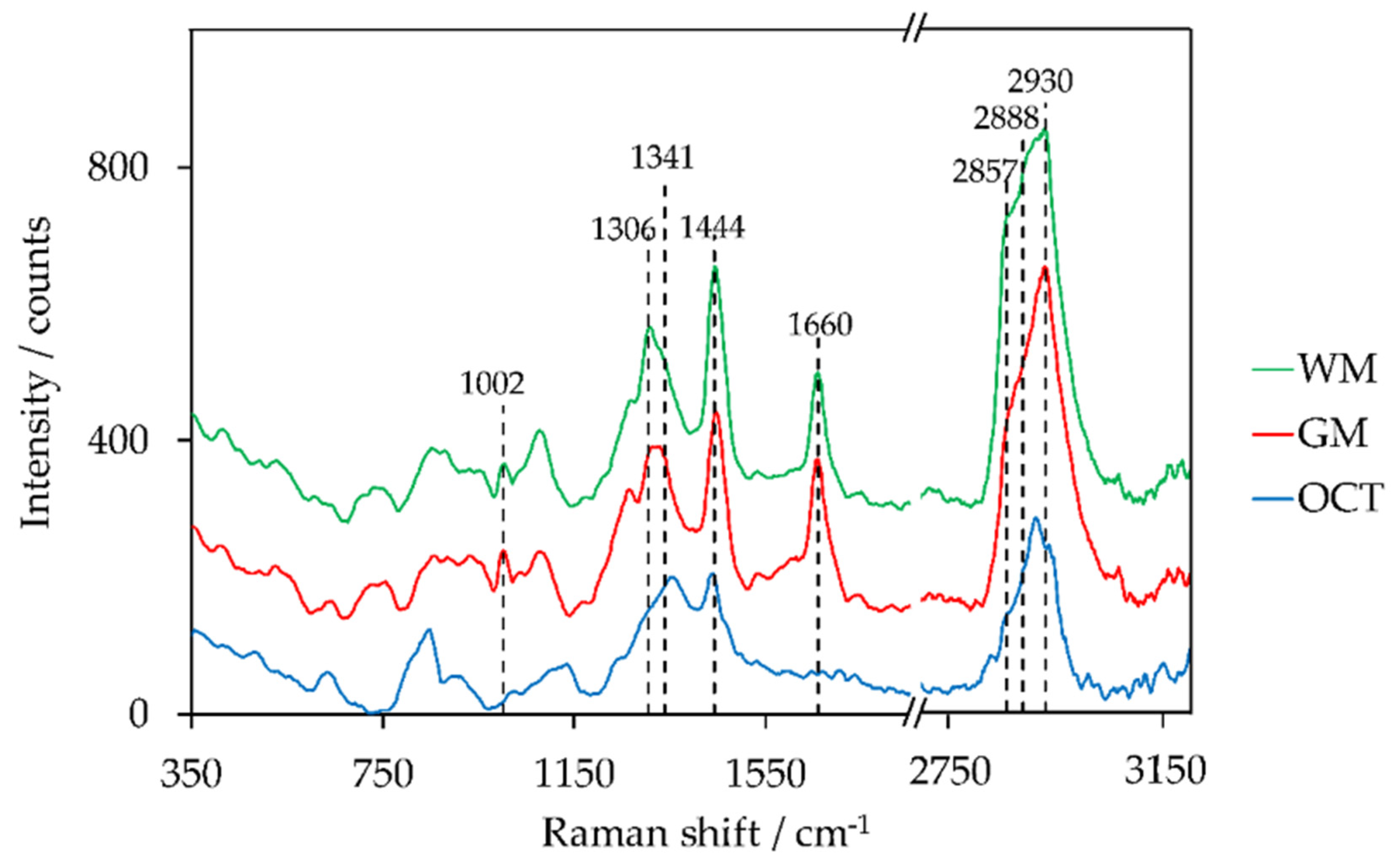
| Peak Position/cm−1 | Lipid Assignments | Protein Assignments | References |
|---|---|---|---|
| 1001–1008 | C-C ring breathing of phenylalanine | [34,46,72] | |
| 1296–1308 | CH2 twisting and wagging | [35,55,73] | |
| 1337–1344 | C-H deformation, C-H bending | [35,73] | |
| 1438–1452 | CH2 bending and scissoring CH3 bending | CH2 bending and scissoring CH3 bending | [34,72,74] |
| 1659–1664 | C=C stretching | Amide I (C=O stretching) | [33,34,46] |
| 2850–2860 | CH2 symmetric stretching | CH2 symmetric stretching | [46,72,73] |
| 2880–2895 | CH2 asymmetric stretching | CH2 asymmetric stretching | [46,72,73] |
| 2929–2937 | CH3 stretching | CH3 stretching | [46,72,73] |
Publisher’s Note: MDPI stays neutral with regard to jurisdictional claims in published maps and institutional affiliations. |
© 2021 by the authors. Licensee MDPI, Basel, Switzerland. This article is an open access article distributed under the terms and conditions of the Creative Commons Attribution (CC BY) license (https://creativecommons.org/licenses/by/4.0/).
Share and Cite
Heintz, A.; Sold, S.; Wühler, F.; Dyckow, J.; Schirmer, L.; Beuermann, T.; Rädle, M. Design of a Multimodal Imaging System and Its First Application to Distinguish Grey and White Matter of Brain Tissue. A Proof-of-Concept-Study. Appl. Sci. 2021, 11, 4777. https://doi.org/10.3390/app11114777
Heintz A, Sold S, Wühler F, Dyckow J, Schirmer L, Beuermann T, Rädle M. Design of a Multimodal Imaging System and Its First Application to Distinguish Grey and White Matter of Brain Tissue. A Proof-of-Concept-Study. Applied Sciences. 2021; 11(11):4777. https://doi.org/10.3390/app11114777
Chicago/Turabian StyleHeintz, Annabell, Sebastian Sold, Felix Wühler, Julia Dyckow, Lucas Schirmer, Thomas Beuermann, and Matthias Rädle. 2021. "Design of a Multimodal Imaging System and Its First Application to Distinguish Grey and White Matter of Brain Tissue. A Proof-of-Concept-Study" Applied Sciences 11, no. 11: 4777. https://doi.org/10.3390/app11114777
APA StyleHeintz, A., Sold, S., Wühler, F., Dyckow, J., Schirmer, L., Beuermann, T., & Rädle, M. (2021). Design of a Multimodal Imaging System and Its First Application to Distinguish Grey and White Matter of Brain Tissue. A Proof-of-Concept-Study. Applied Sciences, 11(11), 4777. https://doi.org/10.3390/app11114777