Design of an On-Grid Microinverter Control Technique for Managing Active and Reactive Power in a Microgrid

Abstract

This paper presents the design and implementation of an on-grid microinverter control technique for managing active and reactive power based on a dq transformation. The system was implemented in a solar microinverter development kit (Texas Instruments—TMDSSOLARUINVKIT). This microinverter has two stages: DC-DC and DC-AC. The DC-DC stage contains an active clamp flyback converter, where the maximum power point tracking (MPPT) of the solar panel is obtained with a current-based incremental conductance algorithm. The DC-AC stage comprises a dual-buck inverter in which voltage-, current-, and phase-tracking control loops are implemented to control the active and reactive power. These techniques were simulated in MATLAB using the proposed mathematical model and experimentally validated in the solar development kit. The results show that the simulated model behaved similarly to the real system, and the control techniques presented good performance. The maximum power point (MPP) of the solar panel was monitored in the DC-DC stage using a current reference provided by the incremental conductance MPPT algorithm and was regulated by a 2P2Z control. The algorithm is robust against continuous changes in irradiance, as it quickly follows the ideal power and continually operates at a point close to the MPP. In addition, the active and reactive power control in the DC-AC stage enables the microinverter to supply the maximum active power. Moreover, the microinverter supplies reactive power according to a defined reference and within the established limits. The proposed mathematical model of the microinverter can be used to design new control techniques and other microinverter topologies. In addition, this active and reactive power-control technique can be implemented in low-power and low-cost microinverters to successfully maintain power quality in small microgrids.

1. Introduction

The depletion of natural resources and environmental degradation are current research topics that have generated great concern today due to their accelerating impacts on climate change. Part of the issue is that the primary generation units that supply the increasing power demand are dependent on non-renewable resources, such as coal, oil, and natural gas. This is why the use of renewable energies close to the loads must be rapidly promoted in order to mitigate the effects of climate change.

Microgrids have been proposed as a way to address this transformation by maximizing the efficiency and flexibility of renewable energy resources. A microgrid is an integrated energy system consisting of interconnected loads and energy resources that are distributed within clearly defined electrical limits, acting as a single controllable entity for the power grid [1,2].

Microgrids are made up of different elements, and distributed generators are essential for their correct operation. These present a challenge in terms of interaction with the grid, where power electronics are vital for the proper operation. Furthermore, distributed generators are usually controlled and connected to the grid through electronic inverters and converters. Thus, the control loop for these devices must guarantee the stability of the system, satisfy the load of the microgrid, and maintain the power quality, such as by controlling the voltage magnitudes and active and reactive power.

In the commercial environment, some microinverters only deliver active power to the electrical grid. However, loads demand active and reactive power, which is essential for some electrical devices, such as motors, as well as inductive and capacitive loads. Consequently, by not performing reactive power compensation, adverse effects are generated for the microgrid, such as high currents and voltage magnitude variations, which may require more electrical infrastructure. Therefore, distributed generators are needed to compensate these effects.

Some examples of active and reactive power control using distributed generation have been proposed in the literature. For instance, in [3], the development of a two-stage control was presented. The first stage was the MPPT strategy, which was based on variable steps with predictive current control. The second stage was an active and reactive power control used to control an on-grid multilevel inverter, which was validated in MATLAB. In [4], an intelligent control algorithm with artificial neural networks was presented for an active and reactive power controller in a photovoltaic generation system connected to the grid. The system consisted of two devices: a DC-DC converter with a maximum power point tracking algorithm and a DC-AC hysteresis inverter; thus, independent control of the active and reactive power was required.

An on-grid photovoltaic inverter installed on the low-voltage side of a distribution network was proposed in [5]. The architecture considered its operation and robustness against network faults. In addition, a two-stage predictive control for the DC link and the inverter was proposed. These controllers were evaluated with mathematical analyses and simulations.

Another study related to active and reactive power control techniques for two-stage on-grid inverters in a photovoltaic system was presented in [6]. In this case, the DC link voltage, active power, and reactive power were successfully controlled with an adaptive-PI and adaptive-sliding-mode controller. The voltage magnitude, voltage phase, and frequency of the power grid were provided by a phase-locked loop (PLL) based on a second-order general integral (SOGI), which presented harmonic immunity, a fast tracking accuracy, and a fast dynamic response.

Other research on power control is found in [7], where a structure was proposed for active and reactive power control in a multi-level modular converter. In this research, the current was decomposed into the $dq$ axes using the Park transform. The components of the $dq$ axes were controlled with a sliding-mode controller (SMC). The q axis component was used to control the active power, and the d axis was used to control the reactive power.

Furthermore, in [8], a control strategy for active and reactive power was proposed for a renewable energy system with an on-grid inverter. The main objective was always to inject the greatest amount of active power and generate sufficient reactive power to maintain stability in the grid. This was achieved with a $dq$ transformation and by determining the current amplitude Iq, which was translated into the amount of reactive power that defined the angle between the voltage and the current of the grid.

More recent research, such as that of [9,10,11], addressed the application of techniques based on the $dq$ transform. The authors of [9] proposed an intelligent controller that used a radial basis function artificial neural network in a single-phase direct quadrant $dq$ frame to control the active and reactive power generated by a nine-level packed E-cell (PEC9) inverter. In [10], simulation results that considered high-power solar and wind generation systems were presented to validate the proposed control. This allowed the regulation of power, voltage, and frequency, as well as the coordination of multiple generation units in microgrids. In [11], a novel $dq$ droop control technique was discussed, which applied DC techniques to AC microgrids based on fixed-frequency inverters using the $dq$ transformation. This control technique allowed accurate active and reactive power sharing without alteration of the frequency of the microgrid. Simulations and hardware in the loop (HIL) were used to demonstrate the effectiveness of the control.

On the other hand, an investigation carried out with a microinverter from Texas Instruments (TI) is found in [12]. In this research, a computational model was made and a description of the microinverter’s hardware was provided, in addition to the calculations used by the flyback and dual-buck controllers.

Additionally, some investigations, such as those of [13,14,15], were based on using an active clamp flyback converter in the DC-DC stage and a dual-buck inverter in the DC-AC stage of the TI microinverter. In [13], the main features were presented, and the performance of the active clamp flyback converter was analyzed; this also showed that this converter could provide zero-voltage switching (ZVS). In [14], problems with the dual-buck inverter were discussed, such as the use of more inductors than in a traditional full-bridge inverter, the decreased power density, and the increased system cost. For this reason, a modified cascade full-bridge dual-buck inverter was proposed. In [15], a new circuit structure and a control method were proposed for a high-power interleaved dual-buck inverter, where zero-cross distortion was eliminated, the current stress of the switch was reduced, and the total harmonic distortion at low output power was decreased.

In this research, a control strategy for managing active and reactive power is implemented based on the $dq$ transformation. The modeling and simulation of the complete system were carried out in MATLAB, and the necessary controllers for the two stages of the microinverter were designed. In the DC-DC stage, the maximum power point of the solar panels is monitored, together with the generation of the current reference, which is given by the incremental conductance algorithm and regulated by a 2P2Z control.

In the DC-AC stage, an anti-windup PI controller is implemented for the DC bus voltage, which follows the desired reference and regulates the active power supplied by the microinverter. Then, a phase-locked loop based on a generalized second-order integrator is used, which is fundamental for calculating the P and Q control. In addition, a 3P3Z current controller is proposed, which follows the reference given by the P and Q control. Finally, a feedback linearization strategy is implemented, which compensates disturbances caused by the grid voltages in the 3P3Z control.

The P and Q control is implemented in the TI solar microinverter development kit (TMDSSOLARUINVKIT). The control delivers the maximum active power and supplies reactive power according to the defined reference and within the established limits. In addition, with the possibility of changing the reference values of the voltage in the DC bus and the power, it allows easy integration with a secondary control in order to carry out the correct power management in a microgrid. The performance of the system is evaluated through different case studies.

The main contributions of this paper can be defined as follows. (1) The mathematical model of the commercial microinverter (TMDSSOLARUINVKIT) allows the design of control techniques in simulations and obtains a similar behavior to that of the dynamics of real equipment, thus ensuring its correct functioning during implementation. (2) Our research demonstrates that the proposed active and reactive power control technique may be used in this experimental microinverter (TMDSSOLARUINVKIT), allowing future research on low-cost commercial microinverters. (3) The implementation of an active- and reactive-power-control technique in a low-power microinverter opens up the prospect of using these controls to maintain power quality in small microgrids.

This paper is organized as follows. The preliminaries and descriptions of the models are presented in Section 2, the numerical simulations and experimental tests are presented in Section 3, and the conclusions and future work are presented in Section 4.

2. Materials and Methods

In this section, the injection system model, which includes a solar panel system and two microinverter stages, is presented. In addition, the design of the DC-DC and DC-AC controllers is included. Finally, the programming tasks are implemented in the microcontroller’s card with all the steps necessary for the proper operation of the system.

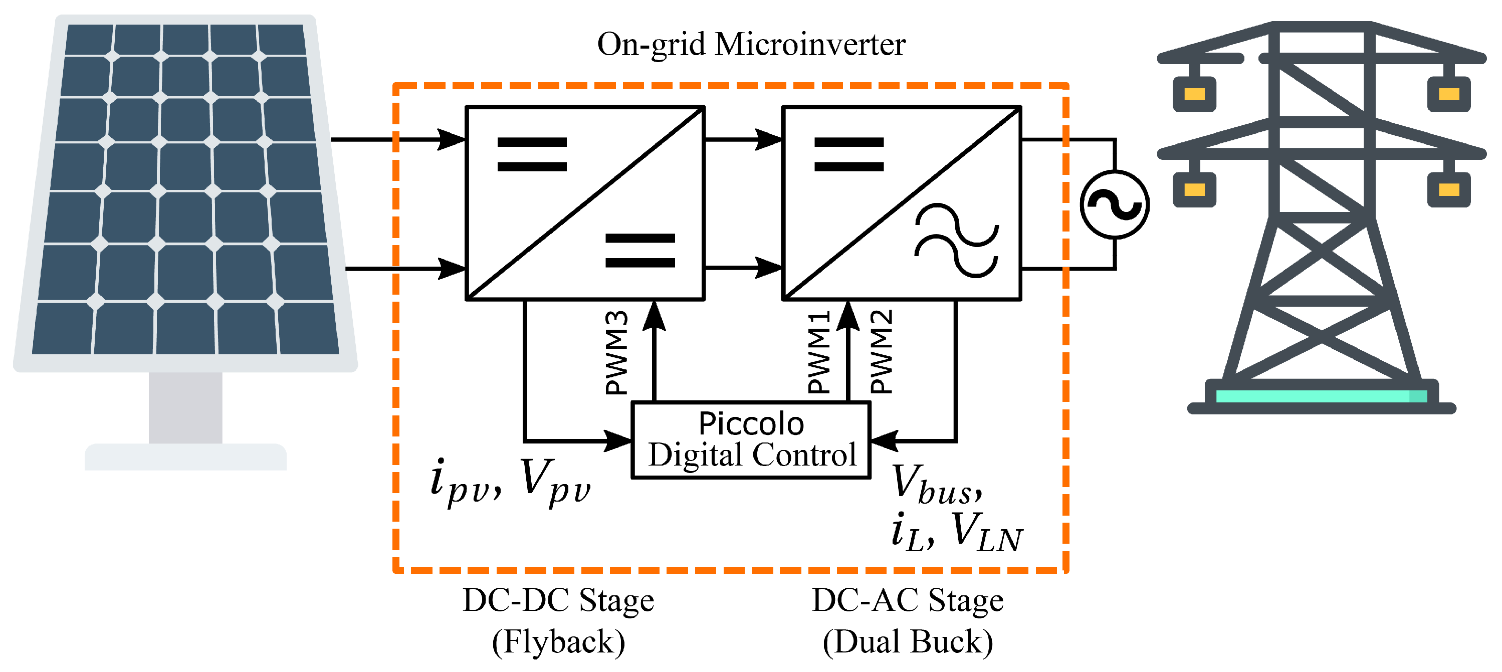
2.1. Model of the Injection System

The design and implementation of the control techniques for managing the active and reactive power were performed with the TI solar microinverter development kit (TMDSSOLARUINVKIT). Figure 1 shows the general diagram of this system. This on-grid microinverter can be divided into two main stages: DC-DC and DC-AC.

In this section, the mathematical formulation of the system is presented in three main parts: solar panel, active clamp flyback, and dual-buck inverter.

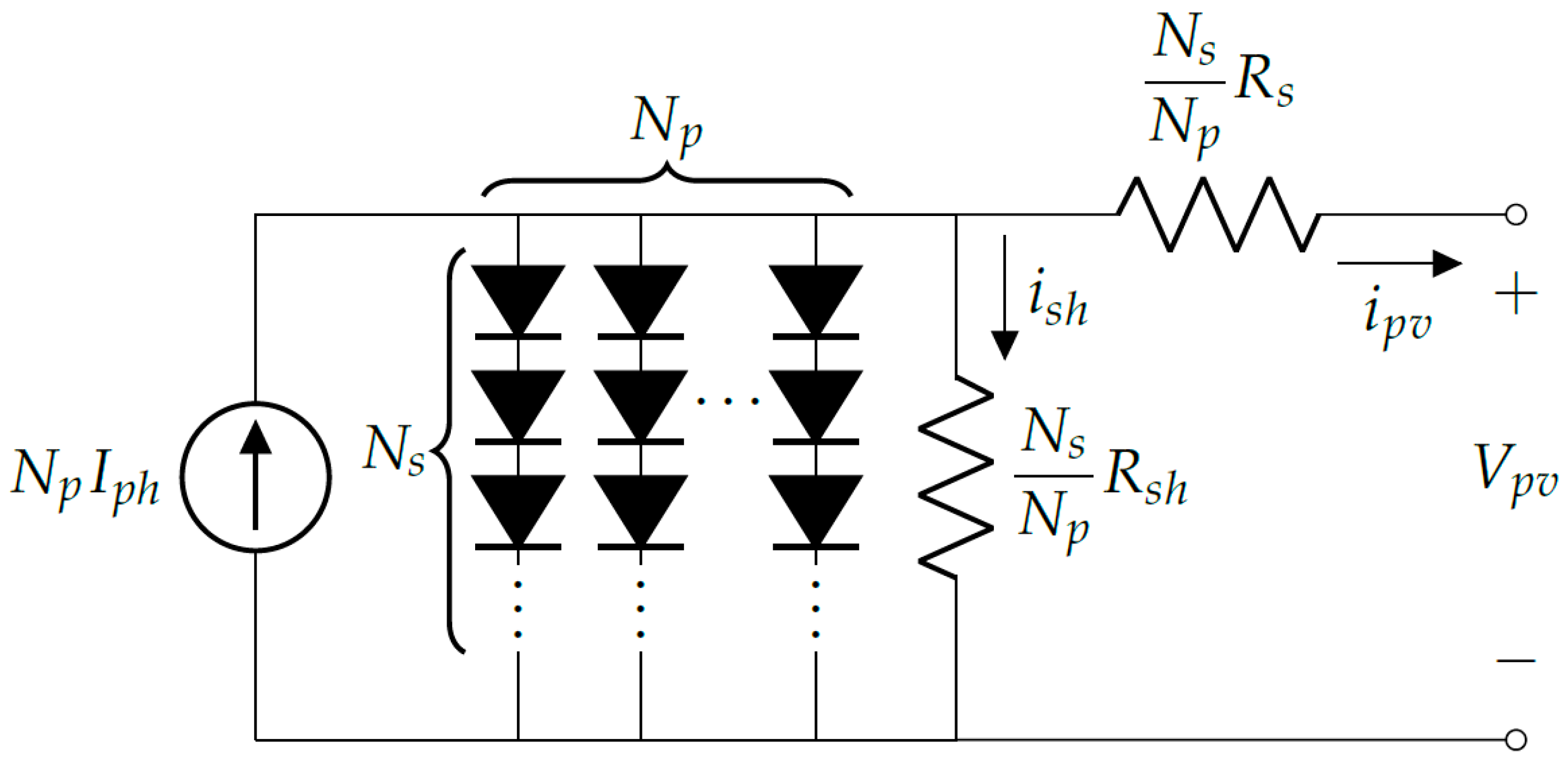
2.1.1. Solar Panel Model

A solar panel is made up of photovoltaic cells in series and in parallel. A model of the equivalent circuit can be seen in Figure 2. Its components are a set of classic pn-junction diodes, which, through the photoelectric effect, convert solar radiation into electrical energy, a current source, and resistive elements that emulate the losses that occur in a real environment [16].

The source $I_{ph}$ is the photogenerated current at a fixed value of solar radiation, the shunt resistance ($R_{sh}$) represents the current loss due to leakage, and the series resistance ($R_s$) is used to represent the voltage drop at the output. Moreover, $N_s$ is the number of cells in series, and $N_p$ is the number of modules in parallel.

The diode current can be written as:

$$I_D=I_s\left[e^{\mathit{\alpha }\left(V_{pv}+R_s{i}_{pv}\right)}-1\right],$$

(1)

where

$$\mathit{\alpha }={\displaystyle \frac{q}{Ak{T}_C}},$$

(2)

where, $k=1.3807\times {10}^{-23}$ JK${}^{-1}$ is the constant of Boltzmann, $q=1.6022\times {10}^{-19}$ C is the charge of the electron, $T_C$ is the operating temperature of the cell in Kelvin, A is the ideality factor of a p-n junction whose value is between 1 and 5, $I_s$ is the saturation current, and $V_{pv}$ is the output voltage of the panel [17]. By applying Kirchhoff’s law and using Equation (1) in the equivalent circuit (Figure 2), the output current ($i_{pv}$) generated by a photovoltaic cell is given by:

$$i_{pv}=I_{ph}-I_s\left[e^{\mathit{\alpha }\left(V_{pv}+R_s{i}_{pv}\right)}-1\right]-{\displaystyle \frac{V_{pv}+R_s{i}_{pv}}{R_{sh}}}.$$

(3)

The photogenerated current $I_{ph}$ depends on the solar irradiance and the cell temperature present in the measurement. It is described by:

$$I_{ph}={\displaystyle \frac{G}{G_{\mathit{ref}}}}\left[I_{sc}+k_i\left(T_C-T_{\mathit{ref}}\right)\right],$$

(4)

where $I_{sc}$ is the short-circuit current, G is the solar irradiance, $G_{\mathit{ref}}=1000$ W/m${}^2$ is the solar irradiance under standard conditions, $k_i$ is the short-circuit current temperature coefficient, and $T_{\mathit{ref}}$ is the working temperature of the cell under normal conditions (298 °K).

The saturation current of the cell $I_s$ changes with temperature [17] according to:

$$I_s=I_{RS}{\left(\frac{T_C}{T_{\mathit{ref}}}\right)}^3{e}^{\frac{q{E}_g}{Ak}\left(\frac{1}{T_{\mathit{ref}}}-\frac{1}{T_C}\right)},$$

(5)

where $E_g$ is the energy of the semiconductor in its forbidden band or bandgap, and $I_{RS}$ is the inverse saturation current of the cell at the reference temperature and solar irradiance, which is given by:

$$I_{RS}={\displaystyle \frac{I_{sc}}{e^{{\displaystyle \frac{v_{oc}}{N_{s}k{T}_{C}A}}}-1}}.$$

(6)

Finally, for $N_s$ photovoltaic cells in series and for $N_p$ modules in parallel, the output current $i_{pv}$ of the panel can be written as:

$$\begin{array}{cc}\hfill i_{pv}& =N_p{I}_{ph}-N_p{I}_s\left[e^{\mathit{\alpha }\left(\frac{V_{pv}}{N_s}+\frac{R_s{i}_{pv}}{N_p}\right)}-1\right]-{\displaystyle \frac{N_p}{R_{sh}}}\left({\displaystyle \frac{V_{pv}}{N_s}}+{\displaystyle \frac{R_s{i}_{pv}}{N_p}}\right).\hfill \end{array}$$

(7)

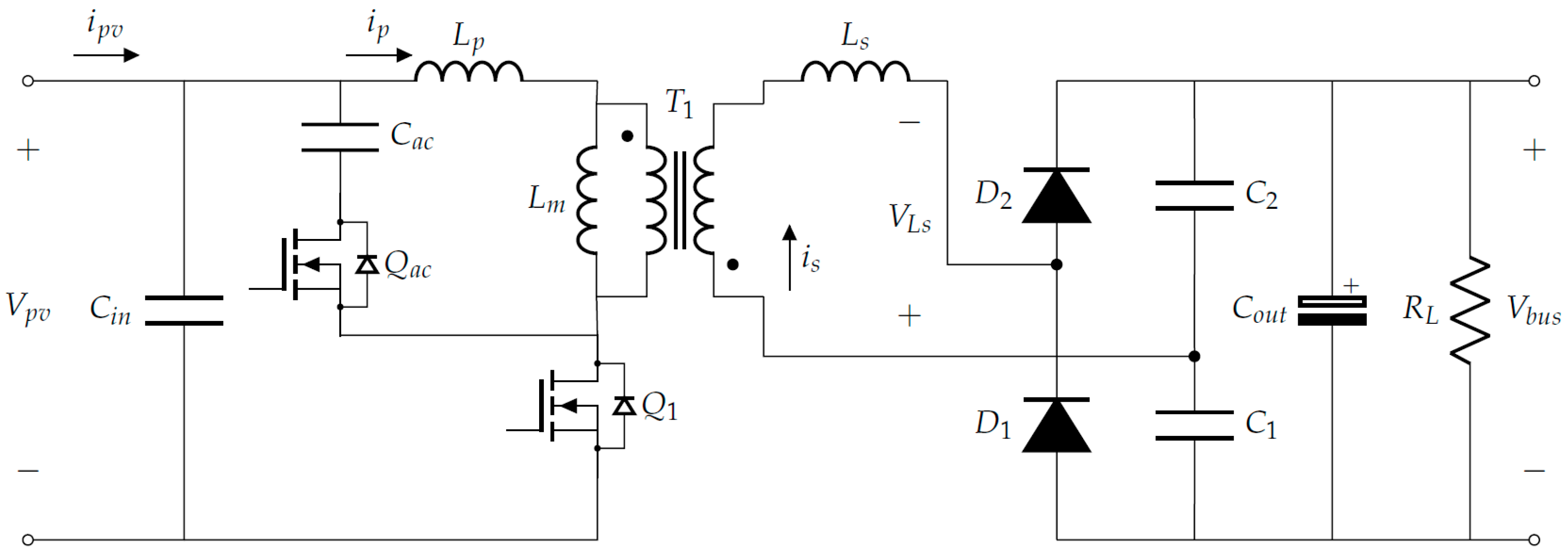
2.1.2. Active Clamp Flyback Model

A DC-DC flyback converter is an isolated version of the buck-boost converter. A transformer is used to eliminate any direct electrical connection (DC) between the input and output of the power converter. Figure 3 shows the active clamp flyback circuit implemented in the TI solar microinverter development kit (TMDSSOLARUINVKIT). The version of the converter with an active clamp (branch $C_{ac}$ and $Q_{ac}$) can provide zero-voltage switching (ZVS), thus reducing switching losses and electromagnetic interference (EMI) and increasing efficiency [13,18].

Furthermore, the capacitor $C_1$ with the diode $D_1$ provides a voltage multiplier circuit at the output of the converter. This multiplier circuit operates in a direct converter mode to transfer energy from the input to the output. From the multiplier, the following is obtained:

$$V_{\mathit{bus}}=-2V_{Ls}.$$

(8)

For modeling, the active clamp stage is omitted, and it is divided into two subintervals.

• Subinterval 1

If $Q_1$ is on, the primary side current increases, the inductance $L_p$ is charged, and energy is stored. On the secondary side, $D_1$ and $D_2$ are off. Therefore, the following equations can be obtained:

$${\displaystyle \frac{d{i}_p}{dt}}={\displaystyle \frac{V_{in}}{L_p+L_m}},$$

(9)

$${\displaystyle \frac{d{V}_{\mathit{bus}}}{dt}}=-{\displaystyle \frac{1}{R_L\left(\frac{C_2}{2}+C_{\mathit{out}}\right)}}{V}_{\mathit{bus}}.$$

(10)

• Subinterval 2

If $Q_1$ is off, power is transferred to the secondary side immediately, and the current $i_p$ decreases to zero. On the secondary side, if $V_{Ls}<0$, the capacitor $C_2$ is charged through the diode $D_2$, and if $V_{Ls}>0$, the capacitor $C_1$ is charged through the diode $D_1$; therefore, $V_{\mathit{Cout}}$ is charged to $2V_{Ls}$. Then:

$${\displaystyle \frac{d{i}_s}{dt}}=-\frac{V_{\mathit{bus}}}{2L_s},$$

(11)

$$i_s={\displaystyle \frac{C_2}{2}}{\displaystyle \frac{d{V}_{\mathit{bus}}}{dt}}+C_{\mathit{out}}{\displaystyle \frac{d{V}_{\mathit{bus}}}{dt}}+{\displaystyle \frac{V_{\mathit{bus}}}{R_L}}.$$

(12)

From the transformation relation n, it is known that $i_s={\displaystyle \frac{i_p}{n}}$. Therefore, Equations (11) and (12) can be written as:

$${\displaystyle \frac{d{i}_p}{dt}}=-{\displaystyle \frac{n}{2L_s}}{V}_{\mathit{bus}},$$

(13)

$${\displaystyle \frac{d{V}_{\mathit{bus}}}{dt}}={\displaystyle \frac{1}{\frac{C_2}{2}+C_{\mathit{out}}}}\left({\displaystyle \frac{i_p}{n}}-{\displaystyle \frac{V_{\mathit{bus}}}{R_L}}\right).$$

(14)

When the input is $u=V_{in}$ and the state variables are

$$x=\left[\begin{array}{c}{i}_p\\ V_{\mathit{bus}}\end{array}\right],$$

(15)

then, with Equations (9) and (10), the state-space system model for subinterval 1 is:

$$\begin{array}{cc}\hfill A_1& =\left[\begin{array}{cc}0& 0\\ 0& -{\displaystyle \frac{1}{R_L\left(\frac{C_2}{2}+C_{out}\right)}}\end{array}\right],B_1=\left[\begin{array}{c}{\displaystyle \frac{1}{L_p+L_m}}\\ 0\end{array}\right],\hfill \\ \hfill C_1& =\left[\begin{array}{cc}1& 0\end{array}\right],D_1=\left[0\right].\hfill \end{array}$$

(16)

Now, considering Equations (13) and (14), the state-space system model for subinterval 2 is:

$$\begin{array}{cc}\hfill A_2& =\left[\begin{array}{cc}0& -{\displaystyle \frac{n}{2L_s}}\\ {\displaystyle \frac{1}{n\left(\frac{C_2}{2}+C_{\mathit{out}}\right)}}& -{\displaystyle \frac{1}{R_L\left(\frac{C_2}{2}+C_{\mathit{out}}\right)}}\end{array}\right],B_2=\left[\begin{array}{c}0\\ 0\end{array}\right],\hfill \\ \hfill C_2& =\left[\begin{array}{cc}1& 0\end{array}\right],D_2=\left[0\right].\hfill \end{array}$$

(17)

The general model of the system is obtained by using the general notation of the state-space averaging technique [20] as follows:

$$\dot{x}=\left(A_{1}d+A_2{d}^{\prime }\right)x+\left(B_{1}d+B_2{d}^{\prime }\right)V_{in},$$

(18)

$$y=\left(C_{1}d+C_2{d}^{\prime }\right)x,$$

(19)

where $d’=1-d$, and d is the duty cycle.

From Equations (18) and (19), the following expression is obtained:

$$\dot{x}=\left[\begin{array}{c}-{\displaystyle \frac{n(1-d)}{2L_s}}{x}_2+{\displaystyle \frac{V_{in}}{L_p+Lm}}d\\ {\displaystyle \frac{1-d}{n\left(\frac{C_2}{2}+C_{\mathit{out}}\right)}}{x}_1-{\displaystyle \frac{1}{R_L\left(\frac{C_2}{2}+C_{\mathit{out}}\right)}}{x}_2\end{array}\right].$$

(20)

The flyback converter’s inputs are $u={\left[dVin\right]}^T$; therefore, the model found in Equation (20) is non-linear. To find the linearized model around the steady-state points of the system, the following expressions are calculated:

$$\begin{array}{cc}\hfill A& ={\left.{\displaystyle \frac{\partial f(x,u)}{\partial x}}\right|}_{\begin{array}{c}x=x_{ss}\\ u=u_{ss}\end{array}}=\left[\begin{array}{cc}0& -{\displaystyle \frac{n(1-u_{1ss})}{2L_s}}\\ {\displaystyle \frac{1-u_{1ss}}{n\left(\frac{C_2}{2}+C_{\mathit{out}}\right)}}& -{\displaystyle \frac{1}{R_L\left(\frac{C_2}{2}+C_{\mathit{out}}\right)}}\end{array}\right],\hfill \\ \hfill B& ={\left.{\displaystyle \frac{\partial f(x,u)}{\partial u}}\right|}_{\begin{array}{c}x=x_{ss}\\ u=u_{ss}\end{array}}=\left[\begin{array}{cc}{\displaystyle \frac{u_{2ss}}{L_m+L_p}}+{\displaystyle \frac{n{x}_{2ss}}{2L_s}}& {\displaystyle \frac{u_{1ss}}{L_p+Lm}}\\ -{\displaystyle \frac{x_{1ss}}{n\left(\frac{C_2}{2}+C_{out}\right)}}& 0\end{array}\right],\hfill \\ \hfill C& =\left[10\right],D=\left[00\right].\hfill \end{array}$$

(21)

Table 1. Parameters for the flyback.

Parameter	Value
$L_s$	4 μH
$L_p$	0.1 μH
$L_m$	0.632 μH
$C_{ac}$	9.4 μF
$C_{out}$	101.5 μF
$C_2$	1.5 μF
n	5.4
$u_{2ss}$	37.4 V
$x_{1ss}$	8.6 A
$x_{2ss}$	275 V
$u_{1ss}$	0.78

shows the parameters used in the model.

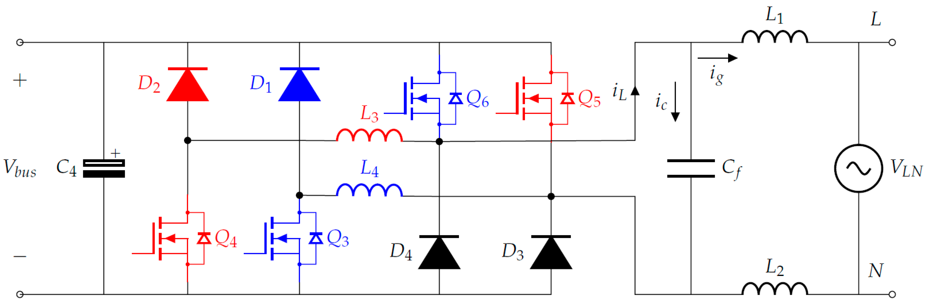
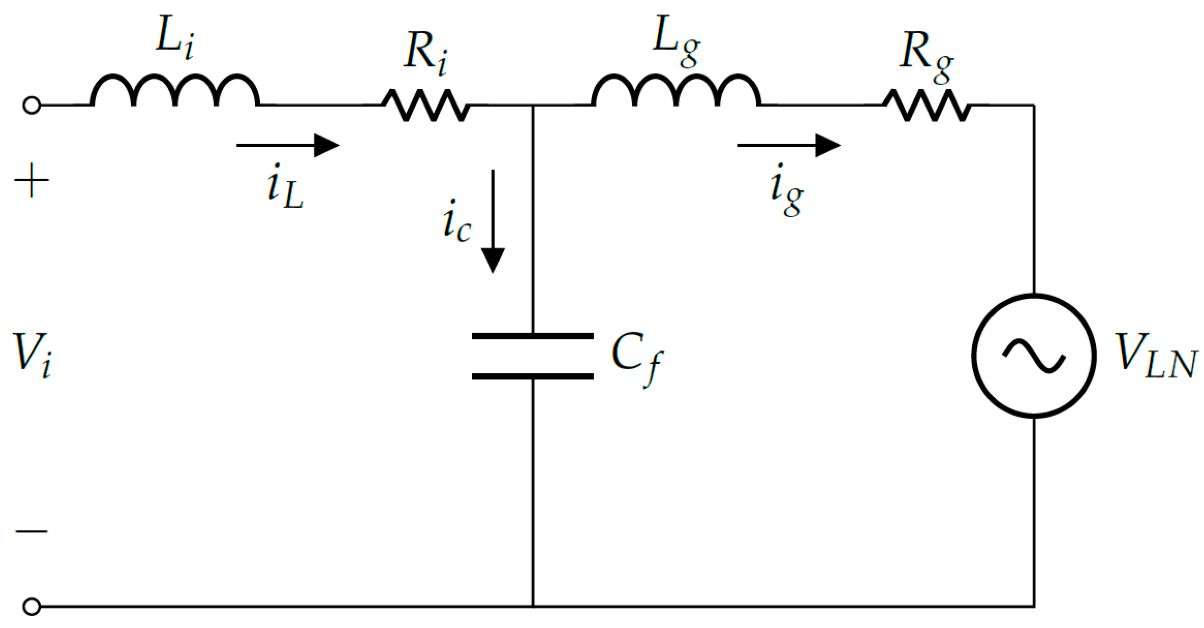
2.1.3. Dual-Buck Inverter Model

The inverter’s output is connected to the electrical grid. The inverter consists of two DC-AC buck converters (Figure 4) operating in one of the half cycles of the line-voltage AC $V_{LN}$. The MOSFETs $Q_6$, $Q_3$, the diode $D_1$, and the inductor $L_4$ make up the first buck converter when $V_{LN}$ is positive. The MOSFETs $Q_5$ and $Q_4$, the diode $D_2$, and the inductor $L_3$ form the second buck converter when $V_{LN}$ is negative. The main inductors, $L_3$ and $L_4$, the capacitor $C_f$, and a second pair of small inductors, $L_1$ and $L_2$, make up an LCL filter at the inverter’s output. In each half cycle, the corresponding upper MOSFET, $Q_6$ or $Q_5$, remains fully on. The lower MOSFETs, $Q_3$ and $Q_4$, operate at a high PWM frequency ($f=50$ kHz) when the buck converter changes in the respective half cycle [19]. Figure 5 summarizes the behavior of the PWMs.

As only one buck converter is active at each half cycle of $V_{LN}$, the model of the circuit can be simplified to that of an LCL filter (Figure 6).

$R_i$ and $R_g$ are the internal resistances of the inductors ($L_i=L_3=L_4$ and $L_g=2L_1$), and $V_{in}$ is the steady-state voltage of the buck converter. Then, $V_i=d{V}_{\mathit{bus}}$, with d as the duty cycle.

Applying Kirchhoff’s voltage and current laws to the LCL filter, the following equations are obtained:

$$V_i=L_i{\displaystyle \frac{d{i}_L}{dt}}+R_i{i}_L+V_C,$$

(22)

$$V_C=L_g{\displaystyle \frac{d{i}_g}{dt}}+R_g{i}_g+V_{LN},$$

(23)

$$i_L=i_c+i_g,$$

(24)

$$i_c=C_f{\displaystyle \frac{d{V}_C}{dt}}.$$

(25)

Therefore, the dynamic behavior of the system is given by:

$${\displaystyle \frac{d{i}_L}{dt}}=-{\displaystyle \frac{R_i}{L_i}}{i}_L-{\displaystyle \frac{1}{L_i}}{V}_C+{\displaystyle \frac{1}{L_i}}Vi,$$

(26)

$${\displaystyle \frac{d{i}_g}{dt}}=-{\displaystyle \frac{R_g}{L_g}}{i}_g+{\displaystyle \frac{1}{L_g}}{V}_C-{\displaystyle \frac{1}{L_g}}{V}_{LN},$$

(27)

$${\displaystyle \frac{d{V}_C}{dt}}={\displaystyle \frac{1}{C_f}}{i}_L-{\displaystyle \frac{1}{C_f}}{i}_g.$$

(28)

Using the following expression as state variables,

$$x=\left[\begin{array}{c}{i}_L\\ i_g\\ V_C\end{array}\right],$$

(29)

and using $u={\left[V_i{V}_{LN}\right]}^T$ as input variables, a linear representation of the system in state space is:

$$\begin{array}{cc}\hfill A& =\left[\begin{array}{ccc}-{\displaystyle \frac{R_i}{L_i}}& 0& -{\displaystyle \frac{1}{L_i}}\\ 0& -{\displaystyle \frac{R_g}{L_g}}& {\displaystyle \frac{1}{L_g}}\\ {\displaystyle \frac{1}{Cf}}& -{\displaystyle \frac{1}{Cf}}& 0\end{array}\right],B=\left[\begin{array}{cc}{\displaystyle \frac{1}{L_i}}& 0\\ 0& -{\displaystyle \frac{1}{L_g}}\\ 0& 0\end{array}\right],\hfill \\ \hfill C& =\left[100\right],D=\left[00\right].\hfill \end{array}$$

(30)

Alternatively, by applying the Laplace transform to Equations (22)–(25), we can obtain the transfer function for $i_L$, which is given by:

$$G_p\left(s\right)={\displaystyle \frac{I_L\left(s\right)}{V_i\left(s\right)-V_{LN}\left(s\right)}}={\displaystyle \frac{b_2{s}^2+b_{1}s+b_0}{a_3{s}^3+a_2{s}^2+a_{1}s+a_0}},$$

(31)

where

$$\begin{array}{cc}\hfill b_0& =1,b_1=C_f{R}_g,b_2=C_f{L}_g,\hfill \\ \hfill a_0& =R_g+R_i,a_1=L_g+C_f{R}_g{R}_i+L_i,\hfill \\ \hfill a_2& =C_f{L}_g{R}_i+C_f{L}_i{R}_g,a_3=C_f{L}_g{L}_i.\hfill \end{array}$$

(32)

Table 2. Parameters of the dual-buck inverter.

Parameter	Value
$L_i$	5.184 mH
$L_g$	940 μH
$R_i$	0.93 $\Omega$
$R_g$	0.26 $\Omega$
$C_f$	0.2 μF

shows the parameters used in the model.

2.2. Design of the DC-DC Controllers

The purpose of the control in the DC-DC stage is to capture the maximum energy from the solar panel. With the solar panel model obtained in Section 2, the power curve at different irradiance points can be obtained (Figure 7). It is observed that the output power is at its maximum only in a single voltage and current point. In addition, this point can change under different atmospheric conditions and solar irradiance.

Therefore, the maximum power point tracking (MPPT) of the panel must be monitored. For this, various MPPT techniques have been developed [21,22,23,24,25,26]. In this research, the incremental conductance algorithm is implemented to achieve this objective, and the scheme is shown in Figure 8. The control loop guarantees that the solar panel current is regulated to the current reference $i_{\mathit{ref}}$ delivered by the MPPT algorithm. This is accomplished by adjusting the duty cycles of the flyback converter’s power MOSFETs. In addition, the proposed scheme includes digital filters for eliminating noise in the current and voltage measurements of the solar panel.

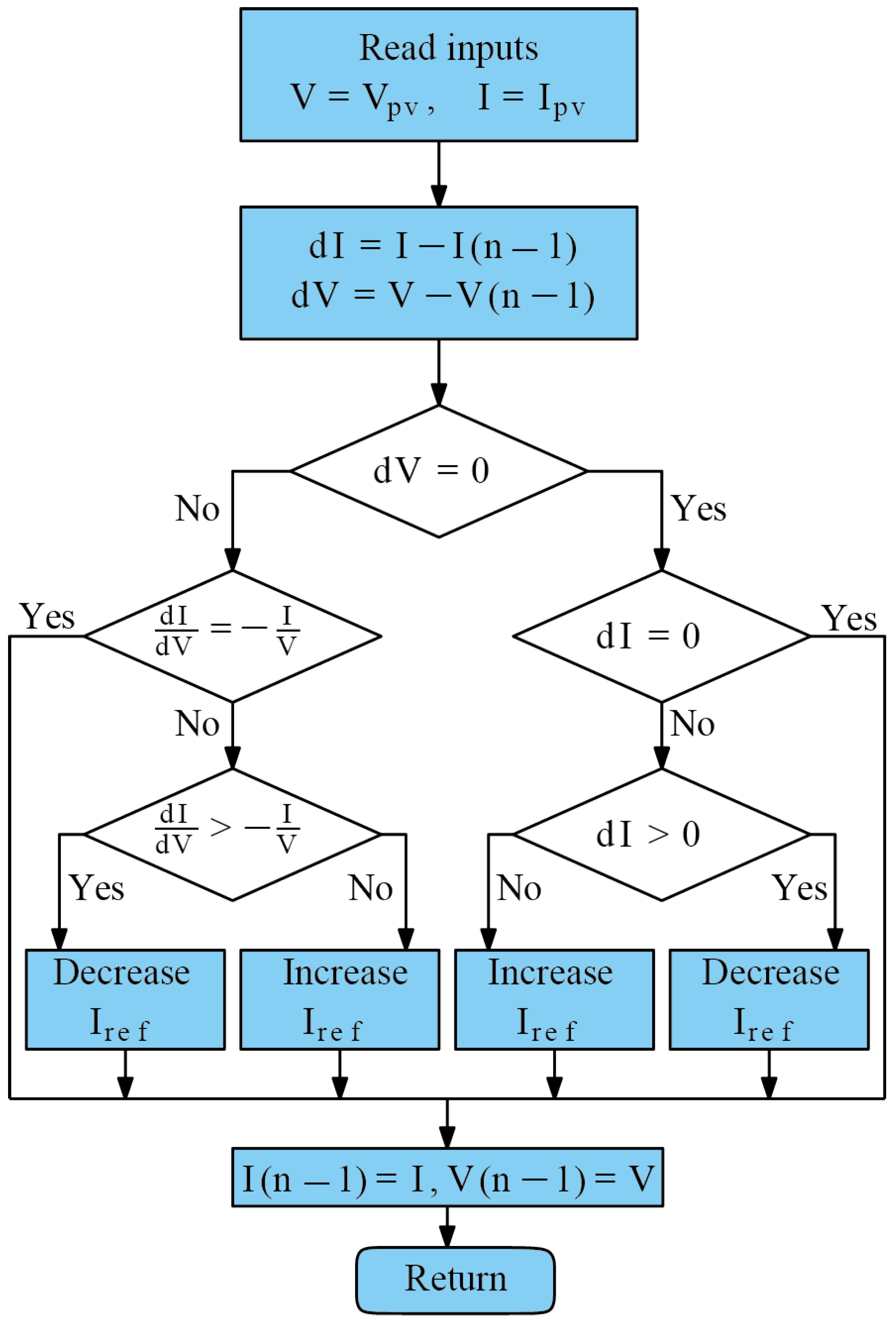
2.2.1. Incremental Conductance MPPT

The incremental conductance algorithm (INCC) shown in Figure 9 takes the voltage $V_{pv}$ and the current $i_{pv}$ of the panel as inputs. Then, it calculates the differentials $dV$ and $dI$. Its operation is based on the fact that the slope of the solar panel power curve is zero at the maximum power point (MPP), positive to the left of the MPP, and negative to the right [27]. From the above, it can be deduced that in the MPP:

$${\displaystyle \frac{dP}{dV}}={\displaystyle \frac{d\left(VI\right)}{dV}}=0,$$

(33)

$$I+V{\displaystyle \frac{dI}{dV}}=0.$$

(34)

Consequently, the following conditions are obtained:

$$\frac{dI}{dV}=-\frac{I}{V},\mathrm{in}\mathrm{MPP};$$

(35)

$$\frac{dI}{dV}<-\frac{I}{V},\mathrm{to}\mathrm{the}\mathrm{right}\mathrm{of}\mathrm{MPP};$$

(36)

$$\frac{dI}{dV}>-\frac{I}{V},\mathrm{to}\mathrm{the}\mathrm{left}\mathrm{of}\mathrm{MPP}.$$

(37)

Therefore, the MPP can be traced by comparing the instantaneous conductance $(I/V)$ with the incremental conductance $(dI/dV)$[19]. Once the MPP is reached, the solar panel’s operation remains at this point unless a change is observed. The algorithm decrements or increments $I_{\mathit{ref}}$ to track the new MPP.

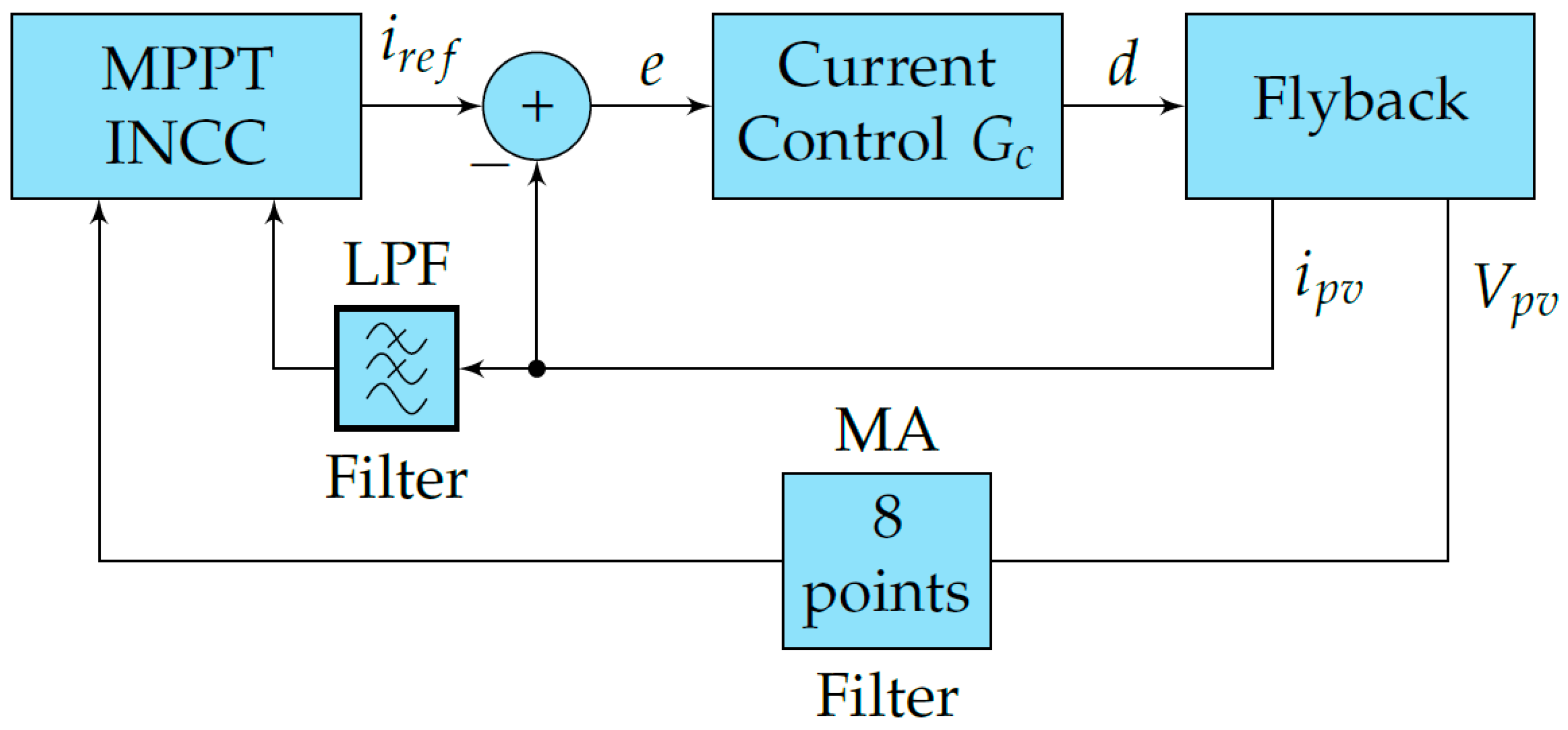
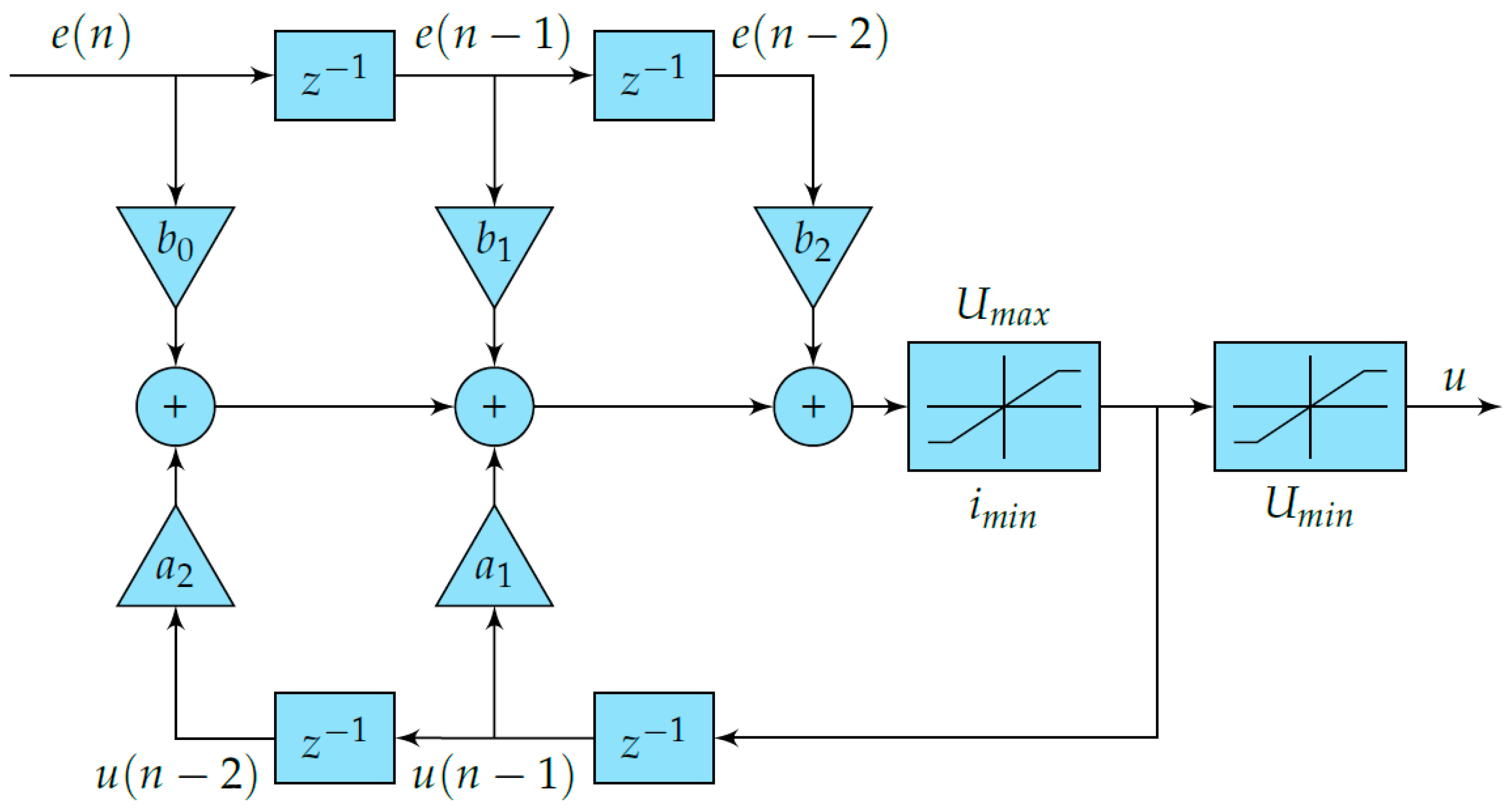
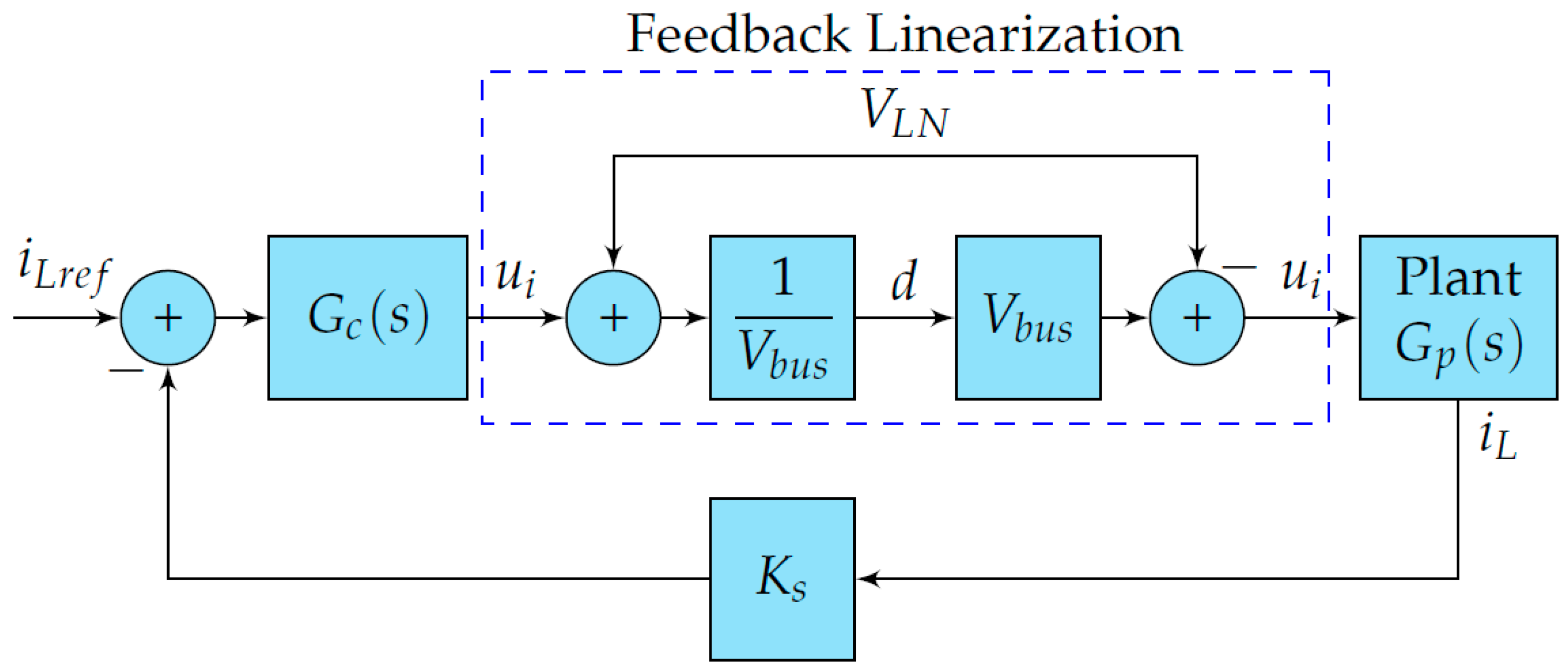
2.2.2. Current Control

For the current control $G_c$, a 2-pole 2-zero compensator (2P2Z) is used. The pulse-transfer function of the 2P2Z control is:

$${\displaystyle \frac{U\left(z\right)}{E\left(z\right)}}={\displaystyle \frac{b_0+b_1{z}^{-1}+b_2{z}^{-2}}{1-a_1{z}^{-1}-a_2{z}^{-2}}}.$$

(38)

If $a_1=1$ and $a_2=0$ are assumed, we can compare them with the pulse-transfer function of a PID, which is given by:

$$\frac{U\left(z\right)}{E\left(z\right)}=\frac{\left(k_P+k_I+k_D\right)-\left(k_P+2k_D\right)z^{-1}+k_D{z}^{-2}}{1-z^{-1}}.$$

(39)

By relating Equations (38) and (39), we obtain:

$$b_0=k_P+k_I+k_D,$$

(40)

$$b_1=-(k_P+2k_D),$$

(41)

$$b_2=k_D.$$

(42)

Using MATLAB and the flyback converter model found in Section 2, the controller is designed, and the constants $k_P=0.0714$, $k_I=0.0203$, and $k_D=0$ are obtained. Therefore,

$$\begin{array}{ccc}{b}_0=0.0917,& b_1=-0.07138,& b_2=0.\end{array}$$

Figure 10 shows the scheme of the 2P2Z controller. $U_{\mathit{max}}=0.8$ and $U_{\mathit{min}}=0$ correspond to the upper and lower limits of the control signal or the duty cycle. The term $i_{\mathit{min}}=-0.05$ is used to have a history of negative values, which can help to avoid oscillations in the output in case there is no load.

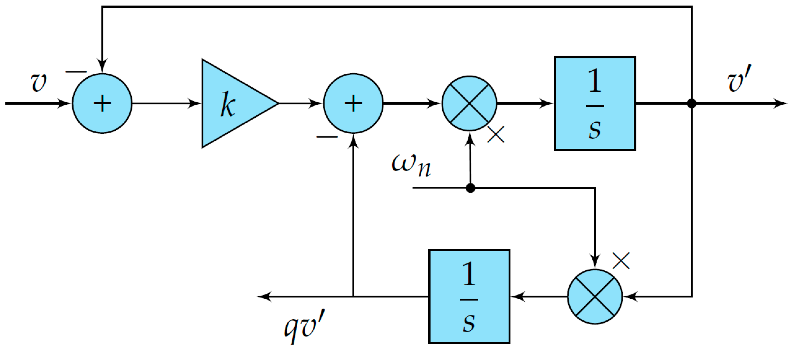
2.2.3. Signal Filtering

The voltage and current values were measured in the solar panel with a SIGLENT SHS1062 oscilloscope and a sampling frequency of 20 kHz at the ADC acquisition points of the microinverter control card.

As the discrete Fourier transform shows that the panel current has high-frequency noise (Figure 11), a Butterworth-type low-pass IIR filter was designed with a cutoff frequency of 115 Hz and order of 2 to eliminate the harmonics from the grid and guarantee high attenuation in high-frequency components. The filter is described by:

$${\displaystyle \frac{U\left(z\right)}{E\left(z\right)}}=k{\displaystyle \frac{b_0+b_1{z}^{-1}+b_2{z}^{-2}}{1+a_1{z}^{-1}+a_2{z}^{-2}}},$$

(43)

where the gain $k=52.25\times {10}^{-6}$ and

$$\begin{array}{cc}\hfill b_0& =1,b_1=2,b_2=1,\hfill \\ \hfill a_0& =1,a_1=-1.97945,a_2=0.97966.\hfill \end{array}$$

An eight-point-average filter was implemented for the panel voltage signal $V_{pv}$ because considerable high-frequency magnitudes were not observed in the Fourier transform. The filter is described by:

$$y\left(n\right)={\displaystyle \frac{1}{8}}\sum _{k=0}^{7}x(n-k).$$

(44)

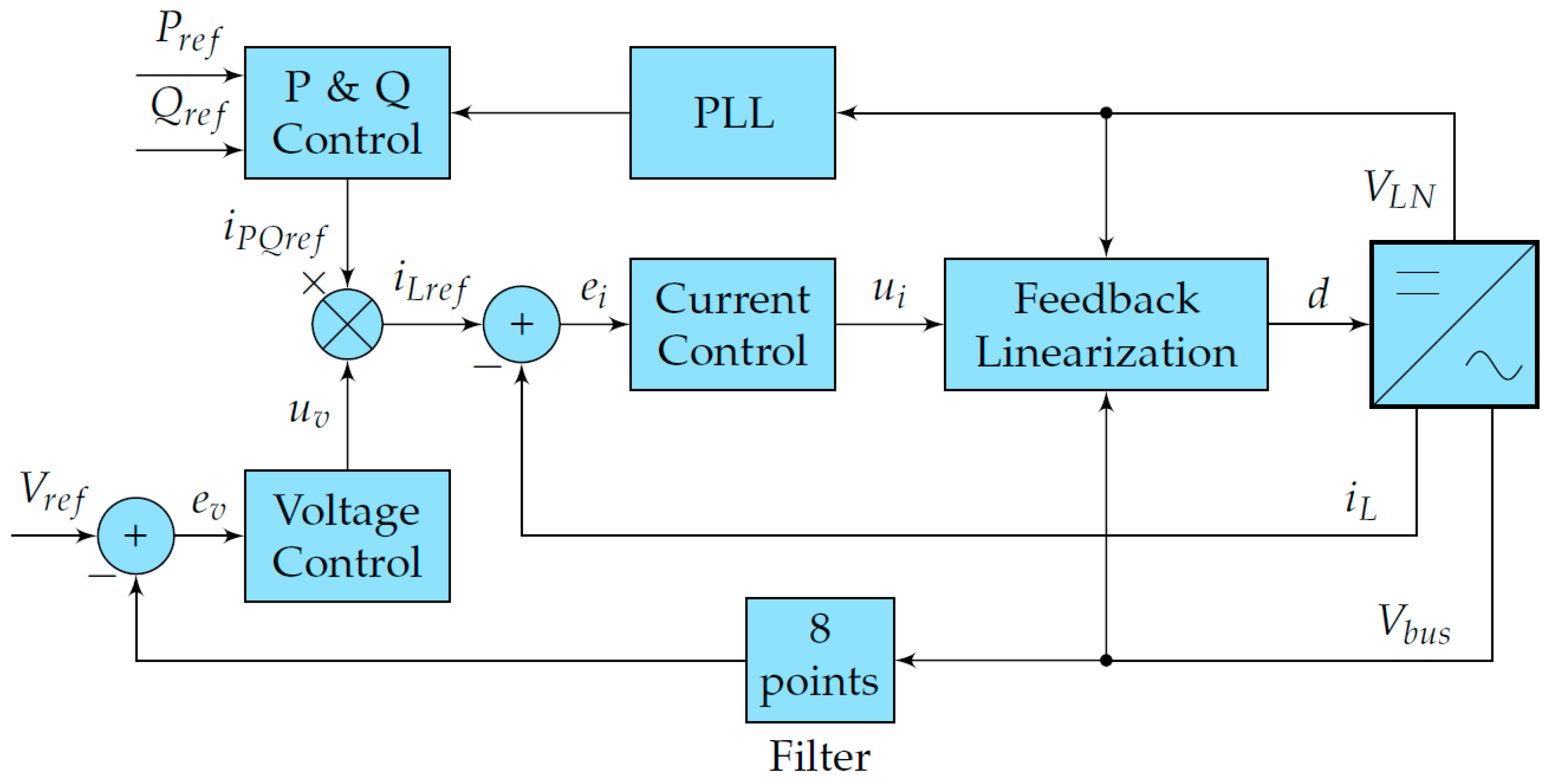
2.3. Design of the DC-AC Controller

The control in the DC-AC stage guarantees synchronization with the electrical grid and the active and reactive power injection with references defined by the user ($V_{\mathit{ref}}$, $P_{\mathit{ref}}$, and $Q_{\mathit{ref}}$). The signals needed to control the DC-AC stage include the line voltage $V_{LN}$, the DC bus voltage $V_{\mathit{bus}}$, and the main inductor current $i_L$. To achieve the effective operation of the inverter, the control scheme in Figure 12 is proposed, where the voltage-control loop is implemented to regulate $V_{\mathit{bus}}$, the current-control loop to regulate $i_L$, and the phase-locked loop (PLL) for active and reactive power control.

2.3.1. Voltage Control (PI)

The voltage-control loop employs an anti-windup PI controller and regulates the input voltage of the DC bus to the reference value $V_{\mathit{ref}}$. The controller output is given by:

$$v_1\left(k\right)=u_p\left(k\right)+u_i\left(k\right),$$

(45)

where $u_p$ and $u_i$ are the proportional part and integral part, respectively. Their values are related in the following way:

$$u_p\left(k\right)=e\left(k\right)=K_p\left[r\left(k\right)-y\left(k\right)\right],$$

(46)

$$u_i\left(k\right)=u_i(k-1)+K_{i}e\left(k\right)w\left(k\right),$$

(47)

where $r\left(k\right)$ is the reference signal, $y\left(k\right)$ is the system output, $K_p$ is the proportional constant, and $K_i$ is the integral constant. The term $w\left(k\right)$ takes values of 1 or 0, providing a means of deactivating the integrator path when output saturation occurs. It prevents the full-term winding up and improves the response time when recovering from saturation [19].

The controller’s output saturates according to the upper ($U_{\mathit{max}}$) and lower ($U_{\mathit{min}}$) limits that are programmable by the user, i.e.:

$$u_v\left(k\right)=\left\{\begin{array}{ccc}{U}_{\mathit{max}}& \mathrm{if}& v_1\left(k\right)>U_{\mathit{max}}\\ U_{\mathit{min}}& \mathrm{if}& v_1\left(k\right)<U_{\mathit{min}}\\ v_1\left(k\right)& \mathrm{if}& U_{\mathit{min}}<v_1\left(k\right)<U_{\mathit{max}}\end{array}\right.$$

(48)

The pre-saturated ($v_1\left(k\right)$) and post-saturated ($u_v\left(k\right)$) terms are compared to determine if saturation is produced, and the following expression finds the value $w\left(k\right)$:

$$w\left(k\right)=\left\{\begin{array}{ccc}0& \mathrm{if}& v_1\left(k\right)\ne u_v\left(k\right)\\ 1& \mathrm{if}& v_1\left(k\right)=u_v\left(k\right)\end{array}\right.$$

(49)

By using MATLAB to implement the inverter model found in Section 2 and adjusting its values with the real system, the constants $K_p=1$ and $K_I=0.001$ are obtained, and the limits $U_{min}=0.025$ and $U_{\mathit{max}}=0.8$ are defined. Additionally, for the voltage signal $V_{\mathit{bus}}$, an eight-point average filter is implemented, as shown in Equation (44).

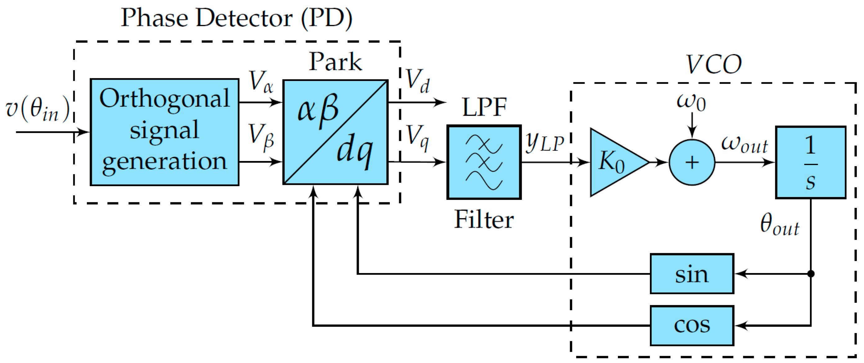
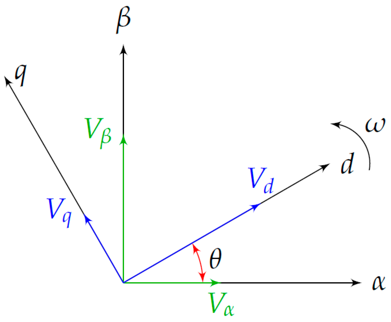
2.3.2. Phase-Locked Loop (PLL)

The PLL is used for synchronizing and monitoring the grid. The phase angle of the grid voltage must be calculated in real time to define the power ratio between the grid and the inverter [28]. In this investigation, the second-order generalized integrator (SOGI)-based phase-locked loop (PLL) is implemented (Figure 13) because it presents harmonic immunity, a fast tracking accuracy, and a rapid dynamic response [6].

The phase detector is composed of an orthogonal signal generator and obtains the Park transform of the waves to detect the components q and d in the rotating reference frame. For the orthogonal signal generator, a second-order generalized integrator (SOGI) [28] is used, as shown in Figure 14. The input signal is the voltage of the power grid. As output signals, two sine waves $v^{\prime }$ and $q{v}^{\prime }$ with a phase shift of $\mathit{\pi }/2$ are generated. The component $v^{\prime }$ has the same phase and amplitude as the input voltage signal $V_{LN}$.

Using the trapezoidal approximation, the closed-loop discrete transfer functions ($Hd\left(z\right)$ and $Hq\left(z\right)$) of the SOGI are:

$$H_d\left(z\right)={\displaystyle \frac{v^{\prime }}{v}}={\displaystyle \frac{b_0-b_0{z}^{-2}}{1-a_1{z}^{-1}-a_2{z}^{-2}}},$$

(50)

$$H_q\left(z\right)={\displaystyle \frac{q{v}^{\prime }}{v}}={\displaystyle \frac{q{b}_0+2q{b}_0{z}^{-1}+q{b}_0{z}^{-2}}{1-a_1{z}^{-1}-a_2{z}^{-2}}},$$

(51)

where

$$\begin{array}{c}\hfill b_0=\frac{x}{x+y+4},q{b}_0=\frac{ky}{x+y+4},\\ \hfill a_1=\frac{2(4-y)}{x+y+4},a_2=\frac{x-y-4}{x+y+4},\end{array}$$

(52)

where $x=2k{\mathit{\omega }}_n{T}_s$, $y={\left({\mathit{\omega }}_n{T}_s\right)}^2$, ${\mathit{\omega }}_n$ is the estimated grid frequency, $T_s$ is the sampling time, and k is the gain that affects the SOGI bandwidth [28].

With the generated orthogonal signal, the Park transform is applied with $V_{\mathit{\alpha }}=v^{\prime }$ and $V_{\mathit{\beta }}=q{v}^{\prime }$ to obtain the components Q and D in the rotating reference frame. The Park transform is given by:

$$\left[\begin{array}{c}{V}_d\\ V_q\end{array}\right]=\left[\begin{array}{cc}cos\left({\mathit{\theta }}_{\mathit{out}}\right)& sin\left({\mathit{\theta }}_{\mathit{out}}\right)\\ -sin\left({\mathit{\theta }}_{\mathit{out}}\right)& cos\left({\mathit{\theta }}_{\mathit{out}}\right)\end{array}\right]\left[\begin{array}{c}{V}_{\mathit{\alpha }}\\ V_{\mathit{\beta }}\end{array}\right].$$

(53)

Defining an arbitrary input signal, $V_{\mathit{\alpha }}=V_{in}cos\left({\mathit{\theta }}_{in}\right)$ and $V_{\mathit{\beta }}=V_{in}sin\left({\mathit{\theta }}_{in}\right)$, the output of the phase detector (PD) is:

$$PD=V_{in}\left[\begin{array}{c}cos({\mathit{\theta }}_{in}-{\mathit{\theta }}_{out})\\ sin({\mathit{\theta }}_{in}-{\mathit{\theta }}_{\mathit{out}})\end{array}\right]=\left[\begin{array}{c}{V}_d\\ V_q\end{array}\right].$$

(54)

Now, assuming that the PLL is synchronized in such a way that ${\mathit{\theta }}_{in}-{\mathit{\theta }}_{\mathit{out}}\approx 0$, then, in $Vq$, we get $sin({\mathit{\theta }}_{in}-\mathit{\theta }\mathit{out})\approx {\mathit{\theta }}_{in}-\mathit{\theta }\mathit{out}$, which is the tracking angle error [19].

Using control theory and using a PI controller as a low-pass filter to keep the error at zero, the closed-loop transfer function of the PLL [28] is given by:

$${\displaystyle \frac{{\mathit{\theta }}_{\mathit{out}}\left(s\right)}{{\mathit{\theta }}_{in}\left(s\right)}}={\displaystyle \frac{k_{p}s+\frac{k_p}{T_i}}{s^2+k_{p}s+\frac{k_p}{T_i}}}.$$

(55)

Now, comparing Equation (55) with the transfer function of a second-order system and defining a settling time of 30 ms, an error band of 5 %, and a damping coefficient of 0.7, we obtain the constants $k_p=166.6$ and $k_i=\mathrm{27,755.55}$.

Finally, using the bilinear transformation, the pulse transfer function of the low-pass filter is given by:

$${\displaystyle \frac{y_{LP}\left(z\right)}{PD\left(z\right)}}={\displaystyle \frac{b_0+b_1{z}^{-1}}{1-z^{-1}}},$$

(56)

where,

$$b_0={\displaystyle \frac{2k_p+k_i{T}_s}{2}}=166.878,$$

(57)

$$b_1={\displaystyle \frac{2k_p-k_i{T}_s}{2}}=-166.322.$$

(58)

2.3.3. Active and Reactive Power Control

For power control, a rotating reference frame is used. Figure 15 shows the stationary and rotating reference frames obtained by performing a $dq$ or Park transformation. The subscripts $d,q$ are components in the rotating reference frame, and $\mathit{\alpha },\mathit{\beta }$ are components in the stationary frame of reference. The term $\mathit{\omega }=\dot{\mathit{\theta }}$ is the angular frequency of the grid [29].

In the rotating reference frame $dq$, the active output power of the inverter [8] can be determined as:

$$P={\displaystyle \frac{1}{2}}\left(V_d{i}_d+V_q{i}_q\right),$$

(59)

where $i_d$, $i_q$, $V_d$, and $V_q$ are the currents and voltages generated on the direct axis (d) and on the quadrature axis (q), respectively. Similarly, the reactive output power injected into the grid is [8]:

$$Q={\displaystyle \frac{1}{2}}\left(V_q{i}_d-V_d{i}_q\right).$$

(60)

From the design of the PLL, it can be deduced that when the rotating frame is synchronized with the grid, $V_q$ is approximately zero. For this reason, the active power control depends on the current component $i_d$ (axis d), while the reactive power control depends on the current component $i_q$ (axis q). Thus, using Equations (59) and (60), we obtain:

$$i_d^{*}={\displaystyle \frac{2P_{ref}}{V_d}},$$

(61)

$$i_q^{*}=-{\displaystyle \frac{2Q_{ref}}{V_d}}.$$

(62)

To guarantee that the maximum active power is always injected into the grid, we define $P_{ref}=P_{\mathit{max}}$ (MPP), assuming that there are no losses [8]. However, the reference voltage $V_{\mathit{ref}}$ of the DC bus can be changed to regulate the active power supplied to the grid.

The current reference in the rotating reference frame, $i_d^{*}$ and $i_q^{*}$, is transformed into the stationary reference frame by using the inverse Park transformation. Furthermore, these variables are regulated by the current control. The inverse Park transform ($dq$⇒$\mathit{\alpha }\mathit{\beta }$) is given by:

$$\left[\begin{array}{c}{i}_{\mathit{\alpha }}\\ i_{\mathit{\beta }}\end{array}\right]=\left[\begin{array}{cc}cos(\mathit{\theta })& -sin(\mathit{\theta })\\ sin(\mathit{\theta })& cos(\mathit{\theta })\end{array}\right]\left[\begin{array}{c}{i}_d\\ i_q\end{array}\right].$$

(63)

In this case, only the real signal needs to be generated, that is, $i_{\mathit{\alpha }}$. Therefore, the current reference given by the active and reactive power control is:

$$i_{\mathit{PQref}}=i_d^{*}cos(\mathit{\theta })-i_q^{*}sin(\mathit{\theta }),$$

(64)

where $\mathit{\theta }$ is the voltage angle of the grid obtained by the PLL.

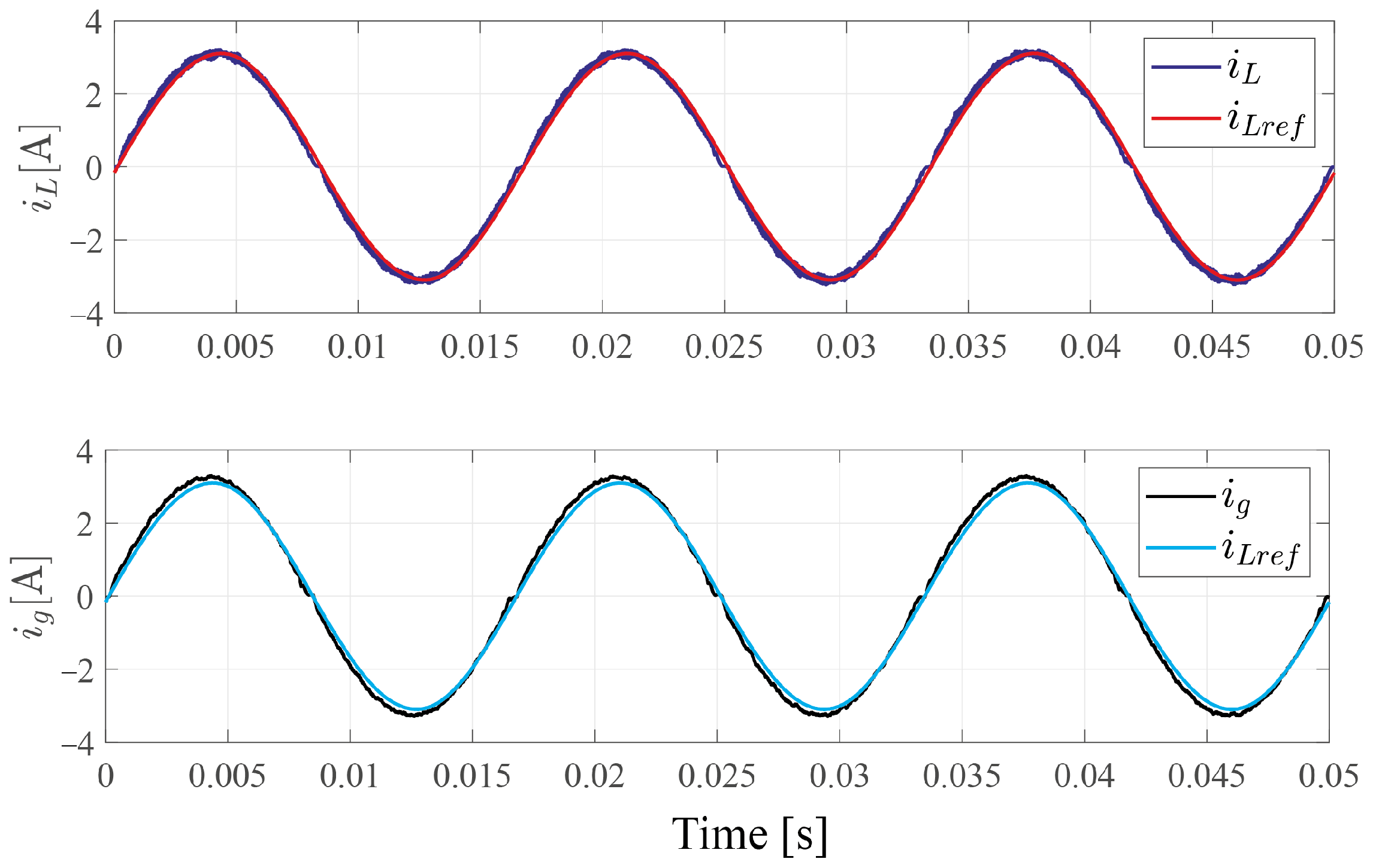
2.3.4. Current Control

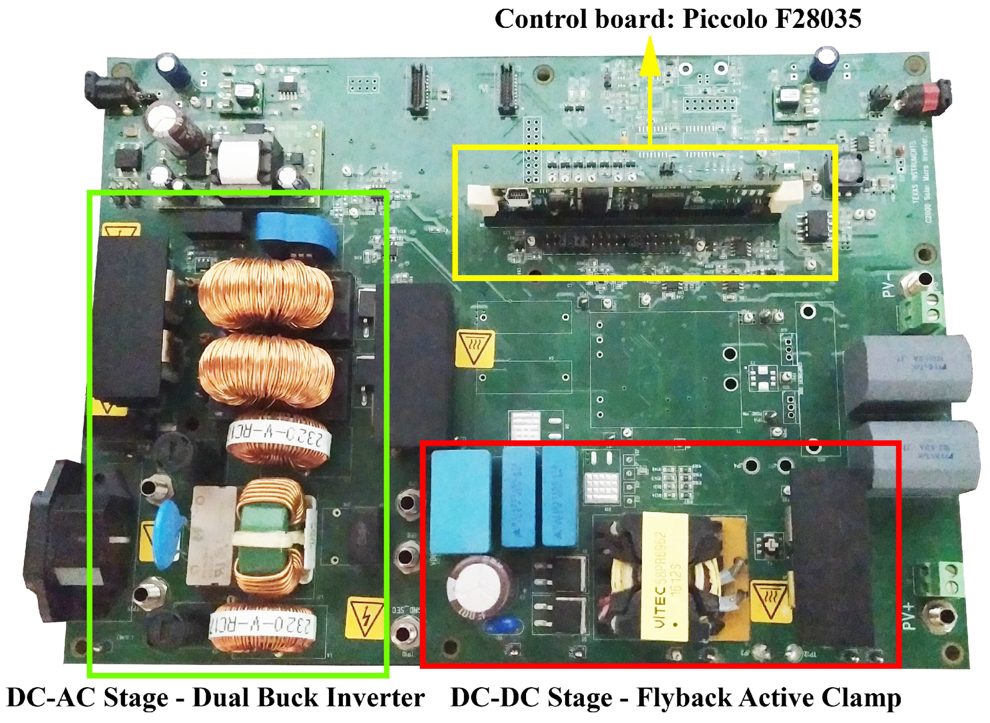
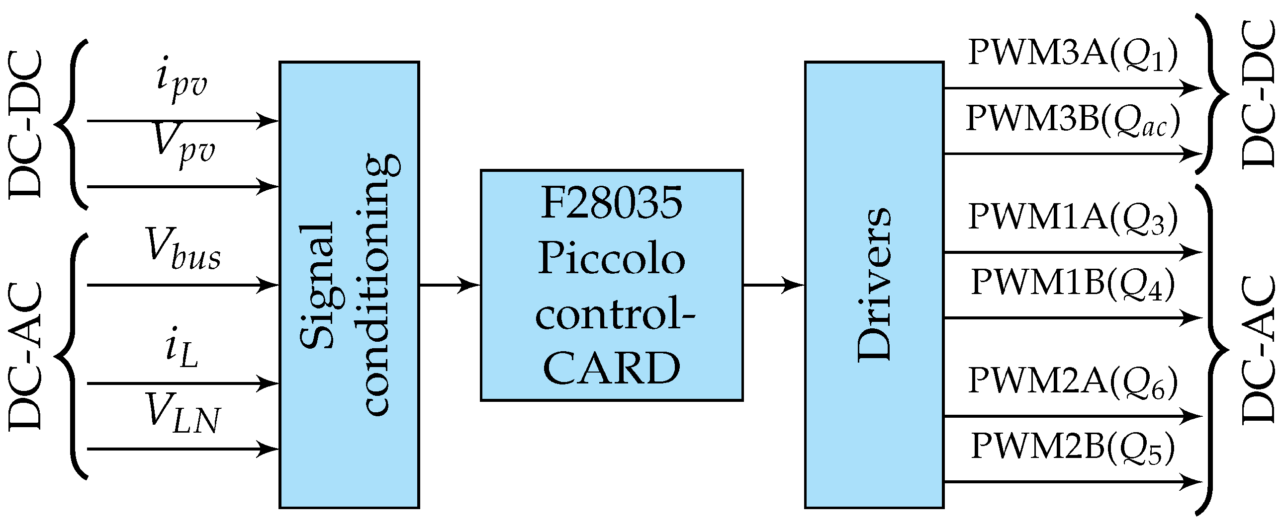
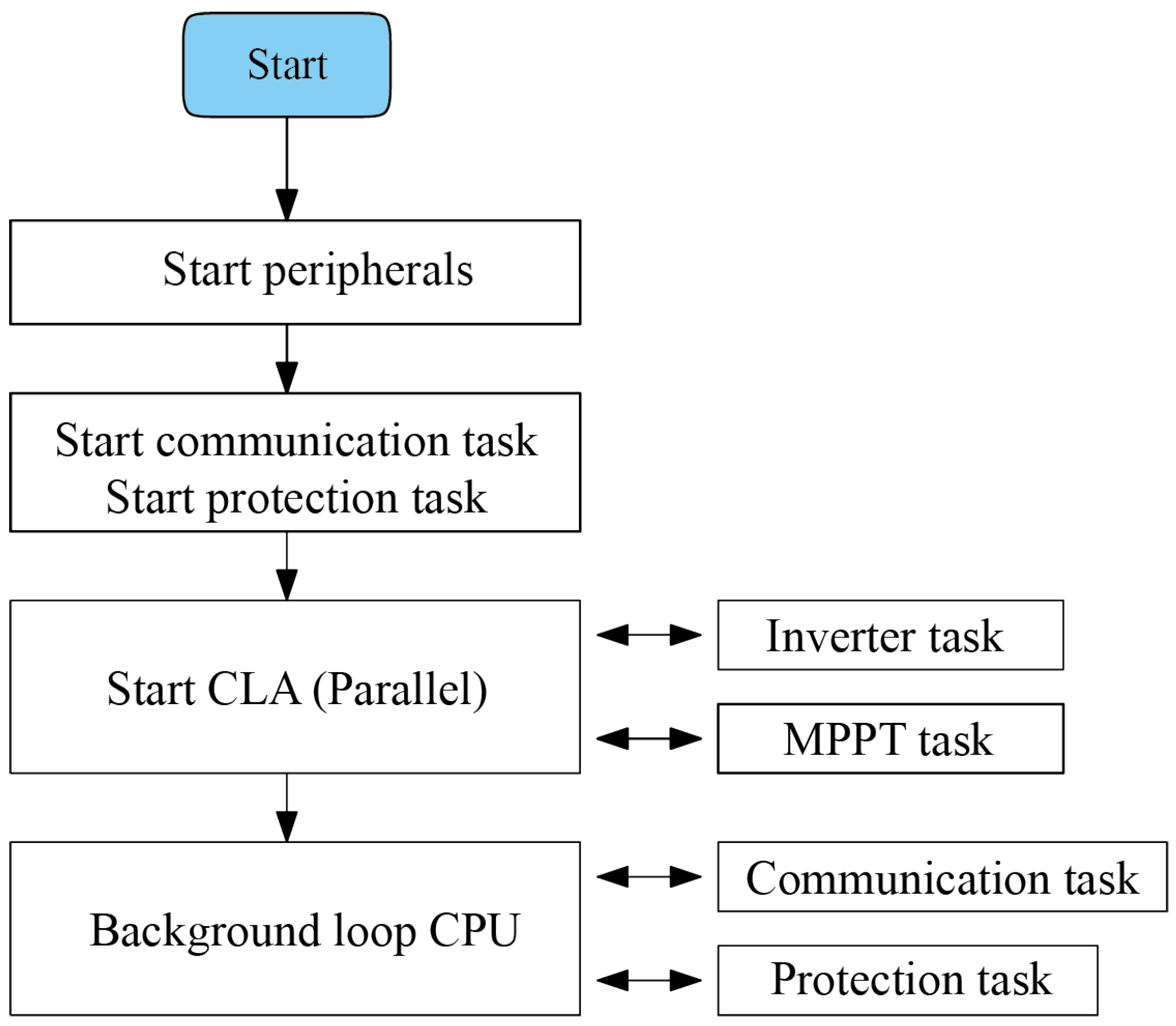
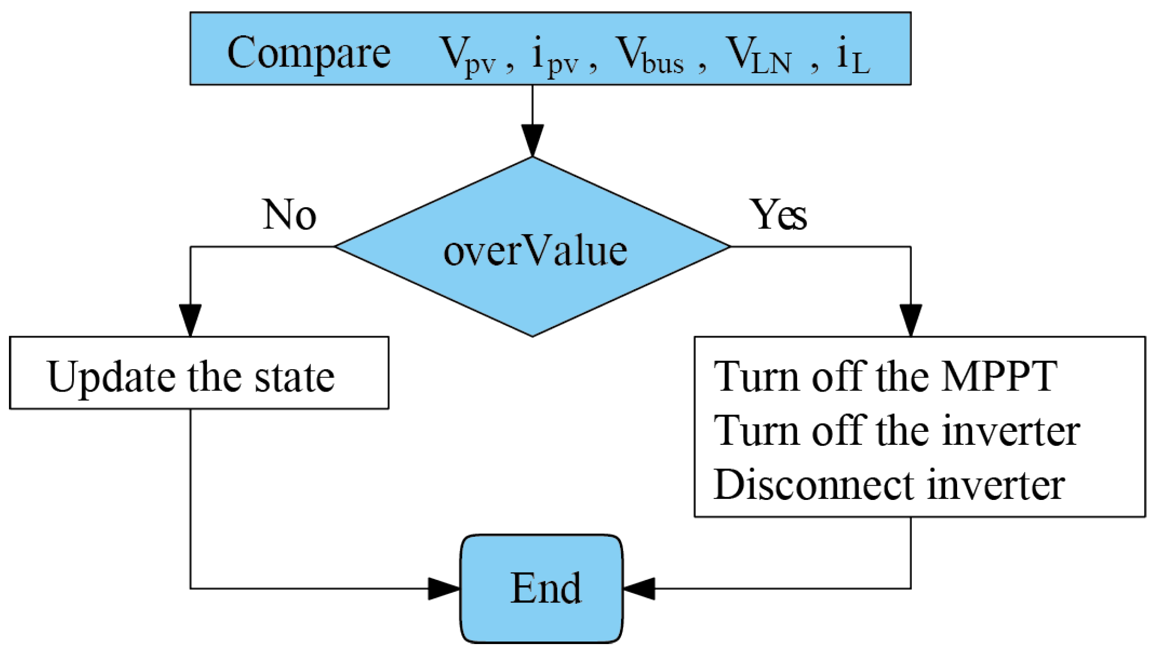
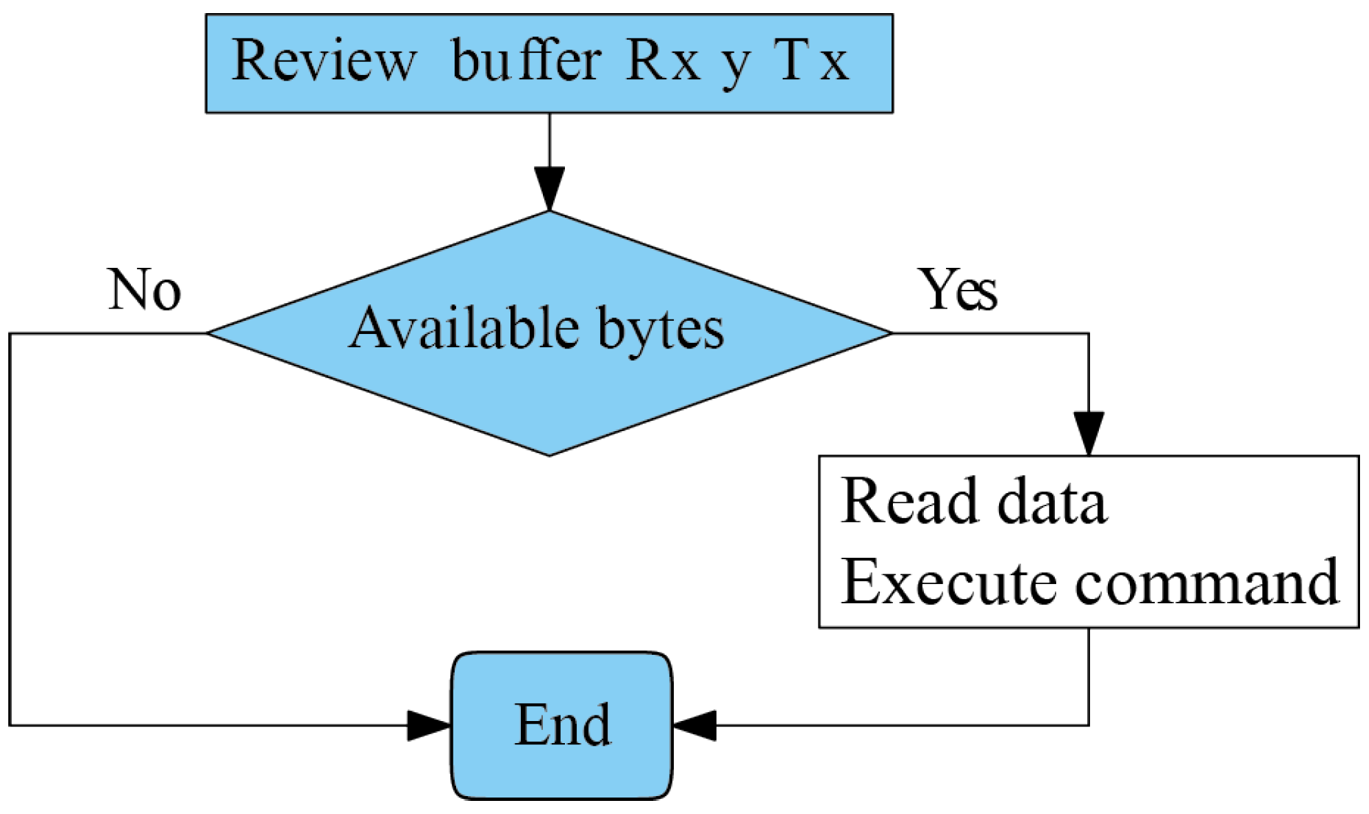
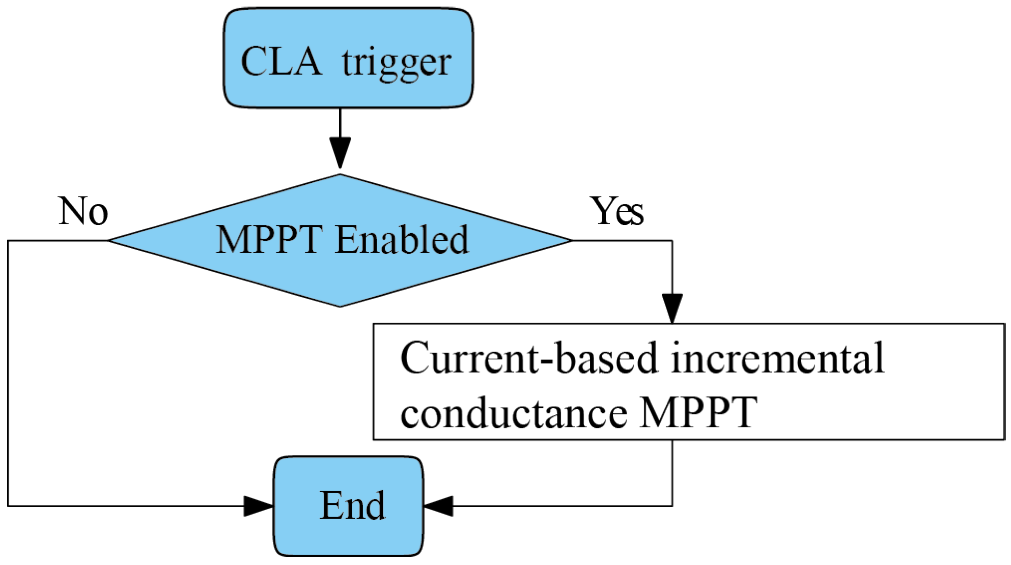
From the transfer function found in Equation (32) of Section 2, it can be seen that the system input is $Vi-V_{LN}=d{V}_{\mathit{bus}}-V_{LN}$, and as $V_{LN}$ is an external input that cannot be controlled, it acts as a disturbance for the current control. To avoid this problem and to be able to calculate the duty cycle (d), a feedback linearization technique is used under the assumption that the cut-off frequency of the current loop is much higher than the grid frequency. Consequently, $V_{LN}$ can be treated as a DC parameter compared to the current dynamics of the inductor $i_L$ [19]. The proposed scheme is shown in Figure 16.

The duty cycle of the PWM that controls the MOSFETs of the inverter is calculated from the feedback linearization as follows:

$$d={\displaystyle \frac{u_i+V_{LN}}{V_{\mathit{bus}}}},$$

(65)

where $u_i$ corresponds to the current control’s output, and $V_{LN}$ and $V_{\mathit{bus}}$ are the measured variables of the inverter.

The following controller is implemented for the $\mathrm{3P3Z}$ current control [19]

$$G_c\left(z\right)={\displaystyle \frac{b_0+b_1{z}^{-1}+b_2{z}^{-2}+b_3{z}^{-3}}{1-a_1{z}^{-1}-a_2{z}^{-2}-a_3{z}^{-3}}},$$

(66)

where

$$\begin{array}{cc}\hfill b_0& =0.2866,b_1=-0.3173,b_2=0.338,b_3=-0.2616,\hfill \\ \hfill a_1& =1.584,a_2=-0.6978,a_3=0.1137.\hfill \end{array}$$

The current reference $i_{\mathit{Lref}}$ is calculated by multiplying the outputs of the PI controllers and the active and reactive power control, that is:

$$i_{\mathit{Lref}}=\left[i_d^{*}cos(\mathit{\theta })-i_q^{*}sin(\mathit{\theta })\right]u_v.$$

(67)

2.4. Implementation

The system was implemented in the TI solar microinverter (Figure 17), which has an active clamp flyback converter, a dual-buck inverter, an F28035 Piccolo controlCARD development board, and conditioning circuits for signal reading. Figure 18 shows the sensed signals and the PWM output necessary to control the microinverter.

The F28035 Piccolo card uses the TMS320F28035 microcontroller from the C2000 line of TI. This card is optimized for processing, sensing, and actuation, thus improving the performance of the control loops for real-time applications, such as industrial motor controllers, solar inverters, electric vehicles, and signal processing. The programming of this card is divided into tasks. In addition, it makes use of parallel processing with a central processing unit (CPU) and the secondary core control law accelerator (CLA), which is a floating-point mathematical accelerator of 32 bits. Figure 19 shows the program initialization process and the creation of tasks that are executed in the CPU and CLA.

One of the essential implementation tasks is protection (Figure 20). This task turns off the microinverter when an overvoltage or overcurrent is presented in any of its sections. This task runs at a frequency of 1 kHz on the main CPU.

When controlling active and reactive power, it is necessary to supply the reference values from an external device, and for this, the UART communication module is used. Figure 21 shows a flow diagram of the communication task.

As current-based MPPT is implemented, it is necessary to run the MPPT algorithm at a lower frequency than that of the 2P2Z compensator to achieve good tracking of the current reference given by the MPPT algorithm. For this case, the MPPT runs at a frequency of 100 Hz, changing the reference of the compensator every 10 ms. Figure 22 shows a flow diagram of the MPPT task.

Finally, the flow diagram of the inverter task is shown in Figure 23; in runs with a 50 kHz frequency to achieve a better control action and synchronize with the grid.

3. Results

With the microinverter and controllers described above, simulation and experimental results were obtained. For power generation, two 150 W solar panels connected in series were used.

Table 3. Parameters of the solar panel (Gi-Power GP-150P).

Parameter	Value
Maximum power, $P_{\mathit{max}}$	150 W
Voltage at maximum power, $V_{mp}$	18.7 V
Current at maximum power, $I_{mp}$	8.02 A
Voltage in open circuit, $V_{oc}$	22.3 V
Short-circuit current, $I_{sc}$	8.51 A

shows the parameters of the solar panel at an irradiance of 1000 W/m${}^2$ and a temperature of 25 ${}^{°}$C [30].

3.1. Simulation Results

The microinverter circuits and components described in Section 2 were simulated using power electronics blocks in MATLAB Simulink. To simulate the solar panel, the “PV-Array” block with the characteristics in Table 3 was used. The controllers were implemented digitally to achieve a better approximation to the real system by using the MATLAB function block. The simulation was carried out in discrete time with a sampling time of 1 $\mathit{\mu }$ s. For the results of the DC-DC stage, the irradiance reference shown in Figure 24 was used to simulate the behavior during the day.

Figure 25 shows the reference generated by the incremental conductance algorithm and the filtered and measured current signals of the panel. It was observed that the 2P2Z control was able to follow the MPPT current reference without steady-state errors, but with some oscillations.

Both the incremental conductance algorithm and current control managed to obtain the maximum power from the solar panel, approaching the ideal power, in the face of continuous irradiance variations. The resulting input power is shown in Figure 26.

In the results of the DC-AC stage, an irradiance reference of 1000 W/m${}^2$ was used. In Figure 27, the response of the 3P3Z current control is shown, where it is evident that the control is capable of following the reference ($i_{\mathit{Lref}}$), but with some oscillations. In addition, the current delivered to the grid—that is, the output current of the LCL filter $i_g$—is shown. The system’s response to the anti-windup PI voltage control (Figure 28) showed oscillations; large parts of these components were eliminated with the digital filter. Furthermore, it was observed that $V_{\mathit{bus}}$ quickly followed the 250 V reference with a settling time of approximately 0.35 s. In this case, the reactive power reference $Q_{\mathit{ref}}$ was set to zero VAR.

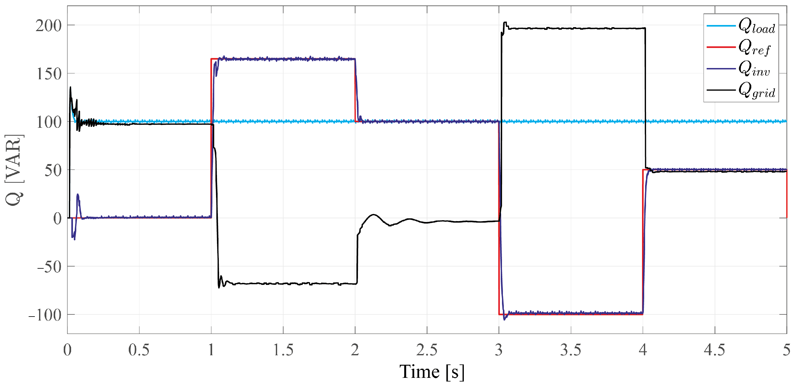
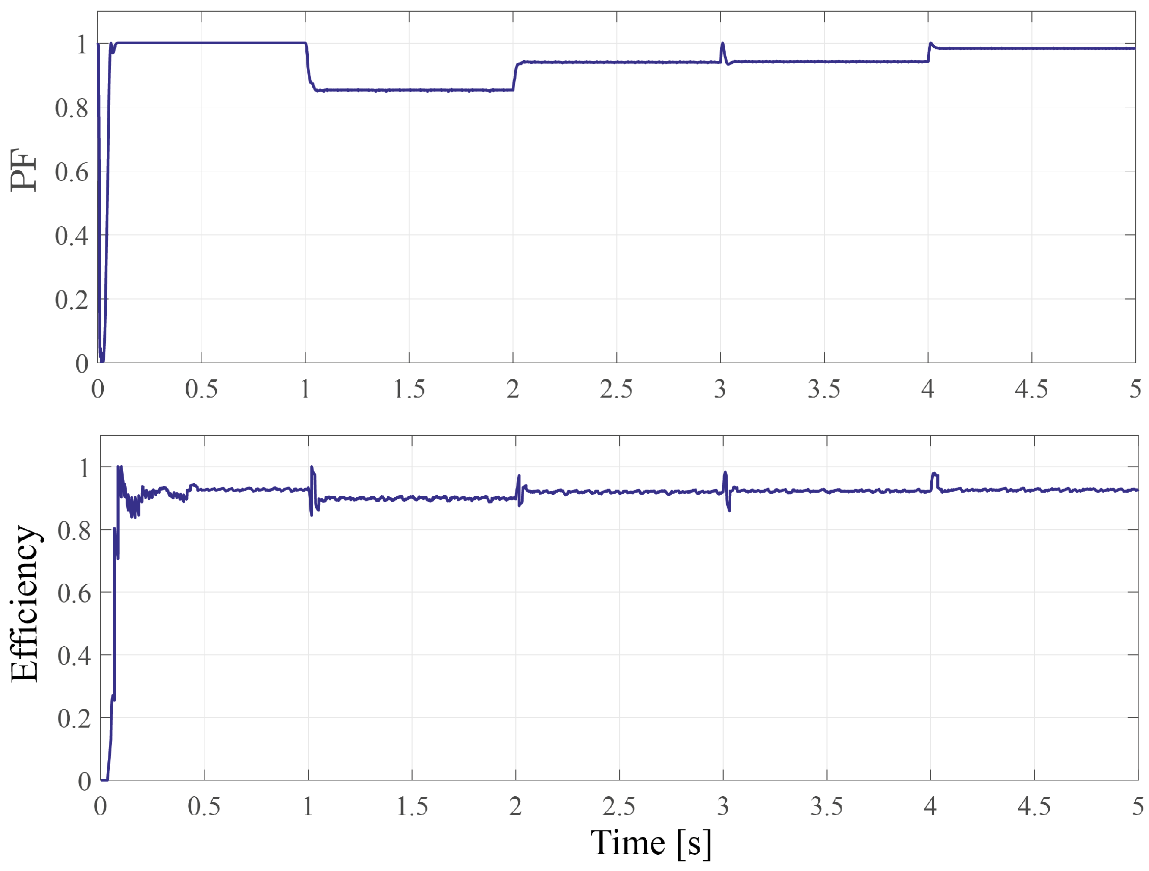
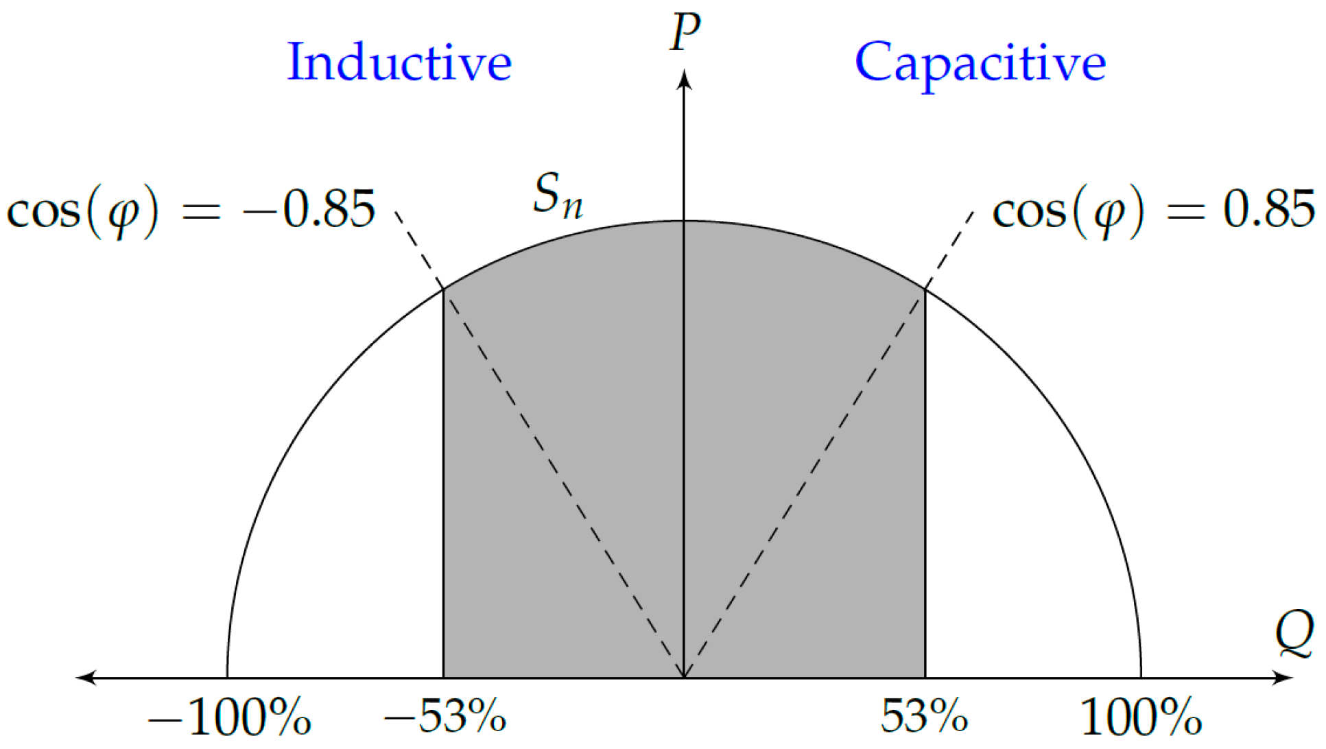
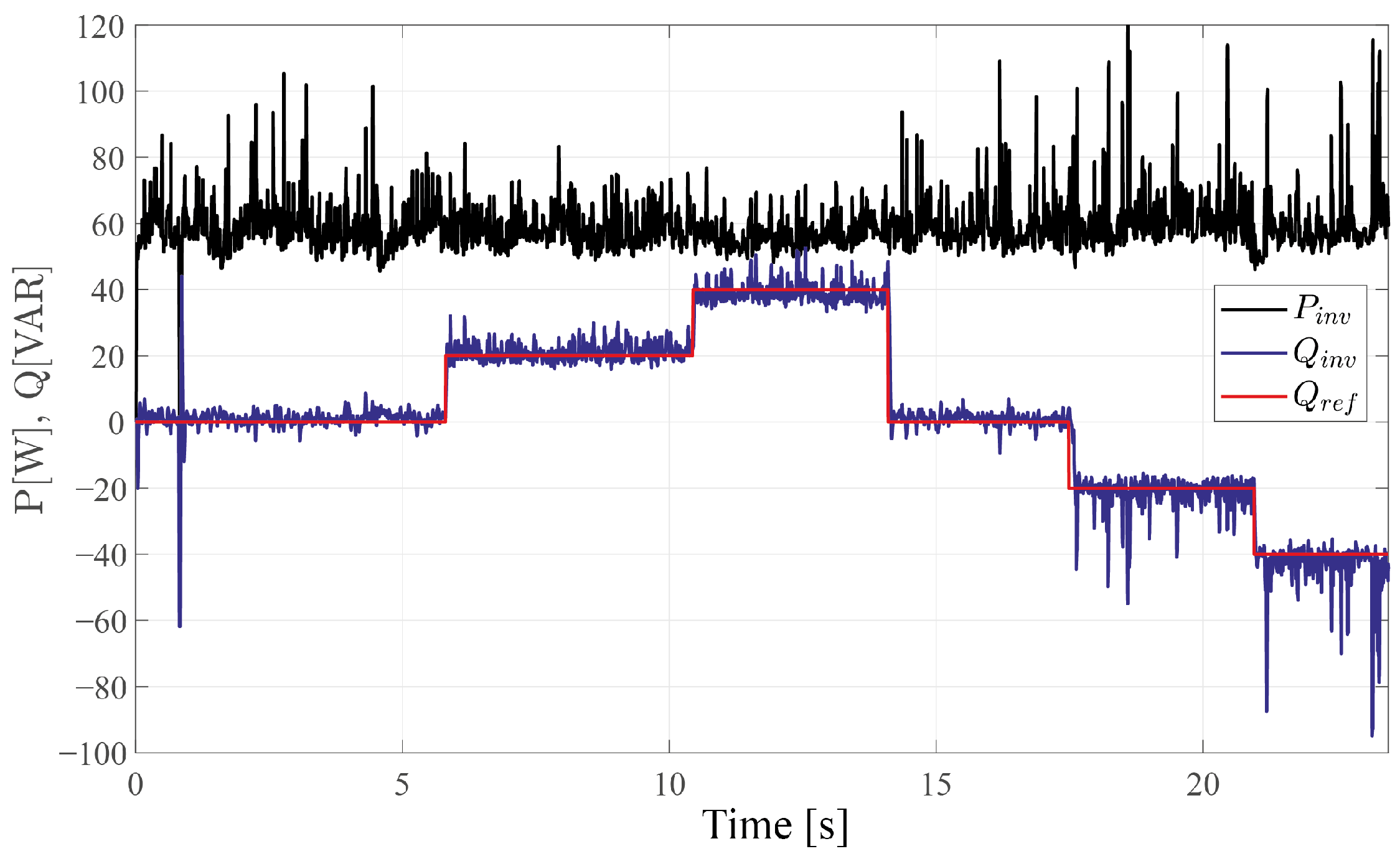
3.1.1. Active and Reactive Power Control

To analyze the process of integrating the inverter with the electrical grid and the active and reactive power control, $P_{\mathit{ref}}$ was established as the power obtained with the MPPT algorithm, and $Q_{\mathit{ref}}$ was set with values of 0, 165, 100, −100, and 50 VAR; the DC bus voltage reference $V_{\mathit{ref}}$ was set to 250 V and was simulated with an irradiance reference of 1000 W/m${}^2$. In addition, a Simulink dynamic load block (single-phase dynamic load) was used, with 280 W and 100 VAR of active and reactive power, respectively.

The maximum possible power was always injected into the grid when $P_{\mathit{ref}}=P_{\mathit{max}}$. In Figure 29, it can be observed that the microinverter was capable of delivering almost all of the power consumed by the load. Therefore, the active power consumption in the grid was reduced to values close to zero. Figure 30 shows the reactive power injected by the microinverter, the reference $Q_{\mathit{ref}}$, the reactive power from the grid, and the reactive power demanded by the load. The P and Q control managed to follow the reference satisfactorily and allowed the generation of both capacitive and inductive reactive power.

Figure 31 shows the phase change of the current with respect to the voltage at the instant in which $Q_{\mathit{ref}}$ changed from 0 to 165 VAR (the power factor changed approximately from 1 to 0.85). It was observed that during the phase shift, there were some oscillations.

In this case, the efficiency and the $TH{D}_i$ were calculated to evaluate the performance of the microinverter. The combined efficiency of the DC-DC and DC-AC stages was, on average, 92 %, which was similar to the efficiency found in [19] and in the experimental results. The minimum $TH{D}_i$ was 2% when $Q_{\mathit{ref}}=0$ VAR, and the maximum $TH{D}_i$ was 5% when $Q_{\mathit{ref}}=165$ VAR (Figure 32). According to the IEEE 1547 standard, the current total harmonic distortion limit for distributed generators is 5% [31]. Therefore, the $TH{D}_i$ values found above were within the suggested range. Furthermore, Figure 33 shows the power factor and the efficiency over time.

On the other hand, it was found that, to guarantee the integrity of the components of the microinverter and maintain the appropriate limits of harmonic distortion, the reactive power reference values must be established within the area shown in Figure 34 with a minimum power factor of ±0.85 or ±53% of the total reactive power.

As these are simulation results, it is possible to define the reactive power reference $Q_{\mathit{ref}}$ that is equal to the measured reactive power of the load to supply the total power demand, as long as it is within the limits defined above. Therefore, the reactive power consumed from the grid is set to zero (Figure 35).

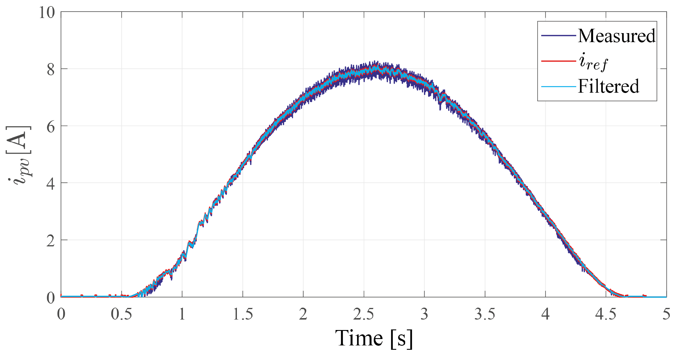
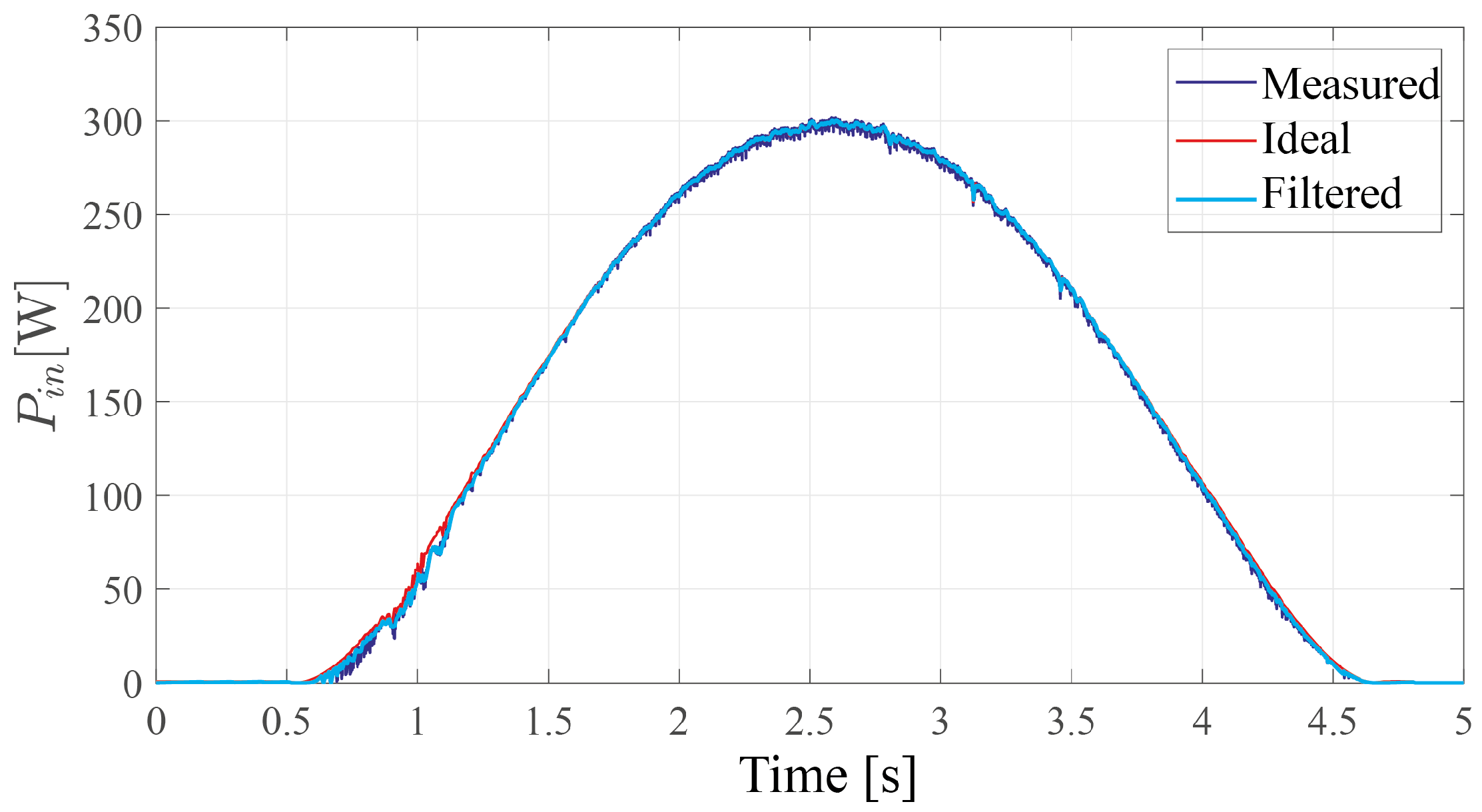
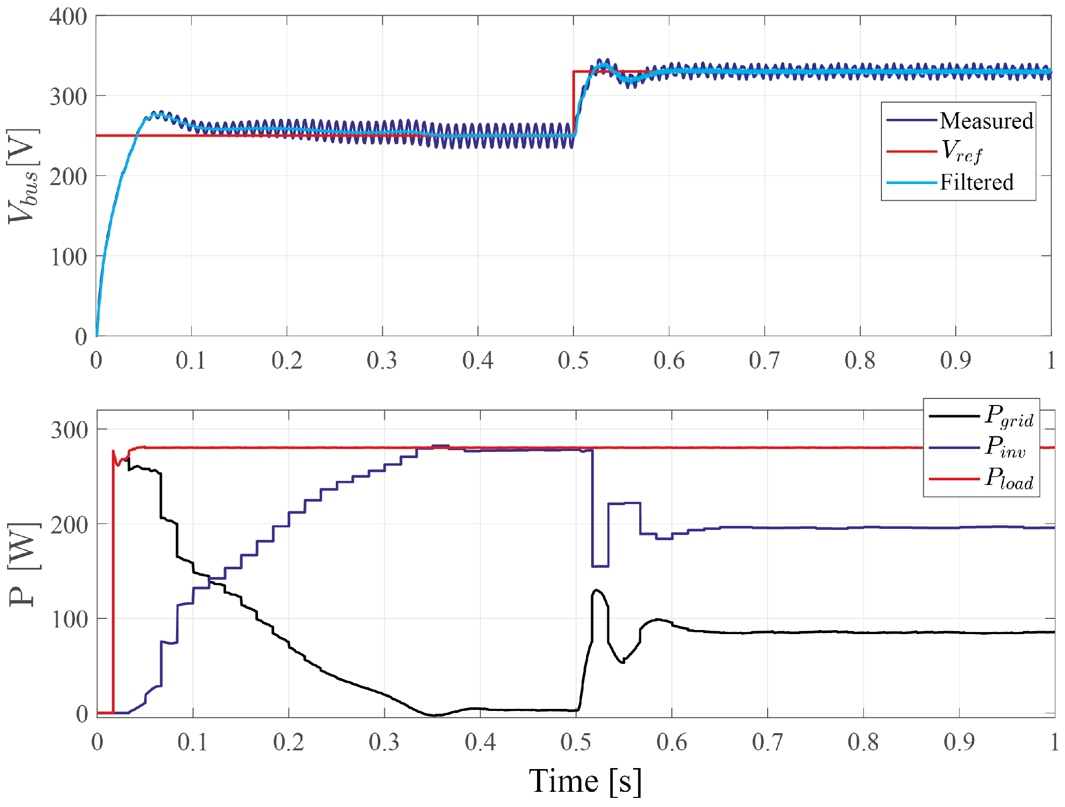
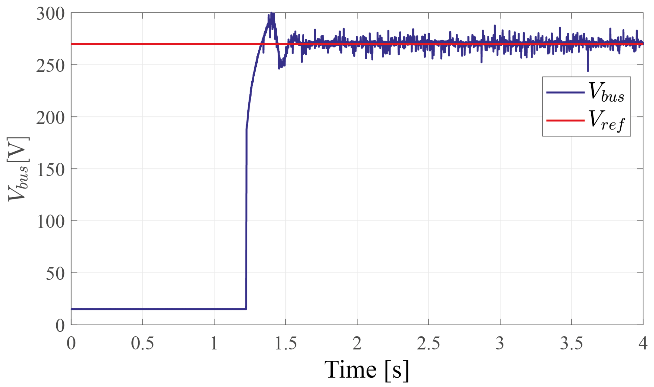
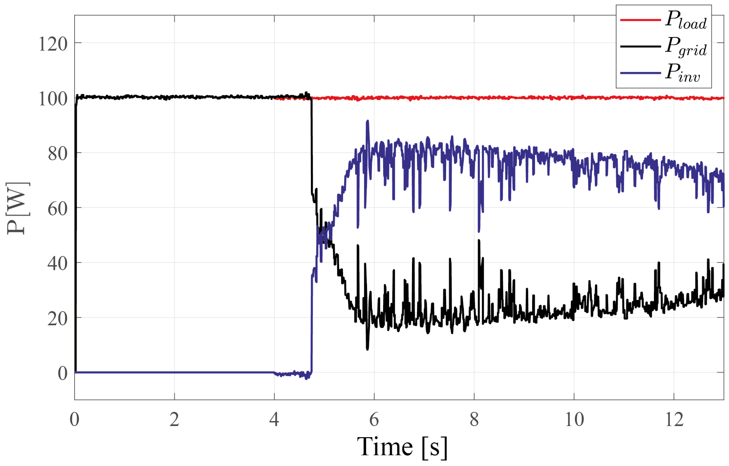
3.1.2. Active Power Regulation

As defined above, $P_{\mathit{ref}}$ must take the value of the maximum power or that obtained by the MPPT. In this case, the maximum power determined was 300 W in order to supply the maximum active power and avoid affecting the dynamics of the reactive power control. However, the active power injected by the microinverter could be regulated by changing the reference voltage of the DC bus $V_{\mathit{ref}}$ within the range of 220 to 380 V (hardware limitations). Figure 36 shows the variation in $V_{\mathit{ref}}$ from 250 to 330 V and the decrease in the active power injected by the microinverter.

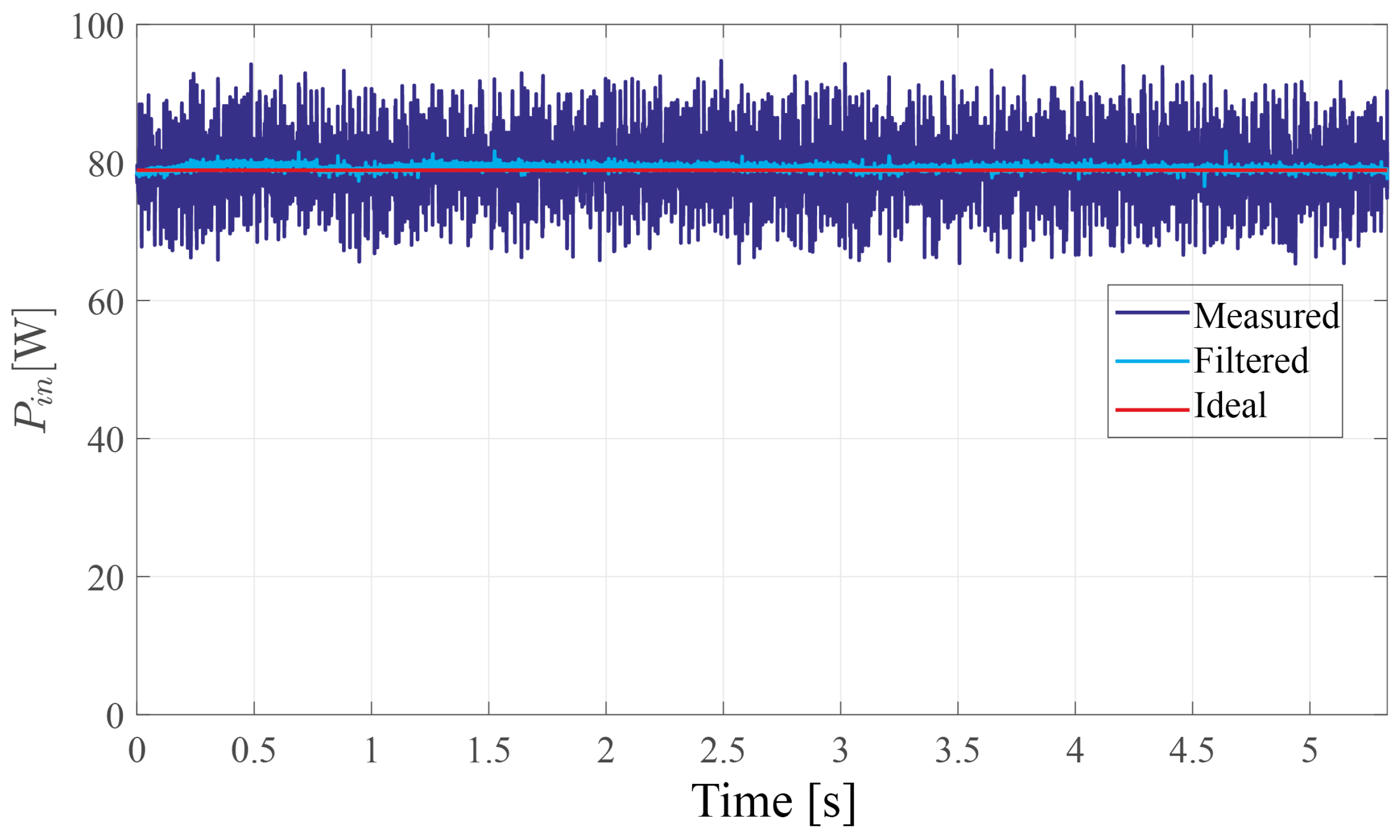
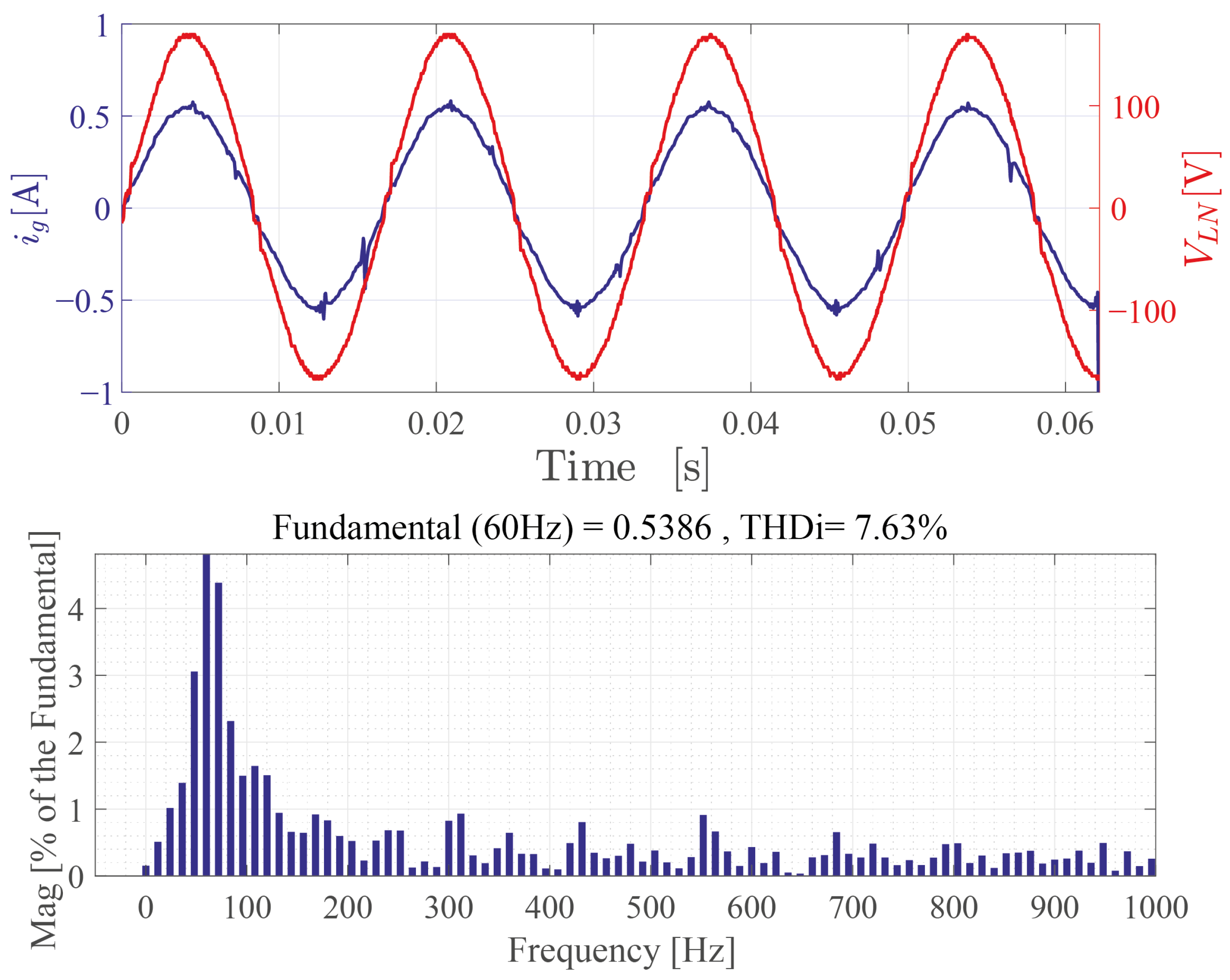
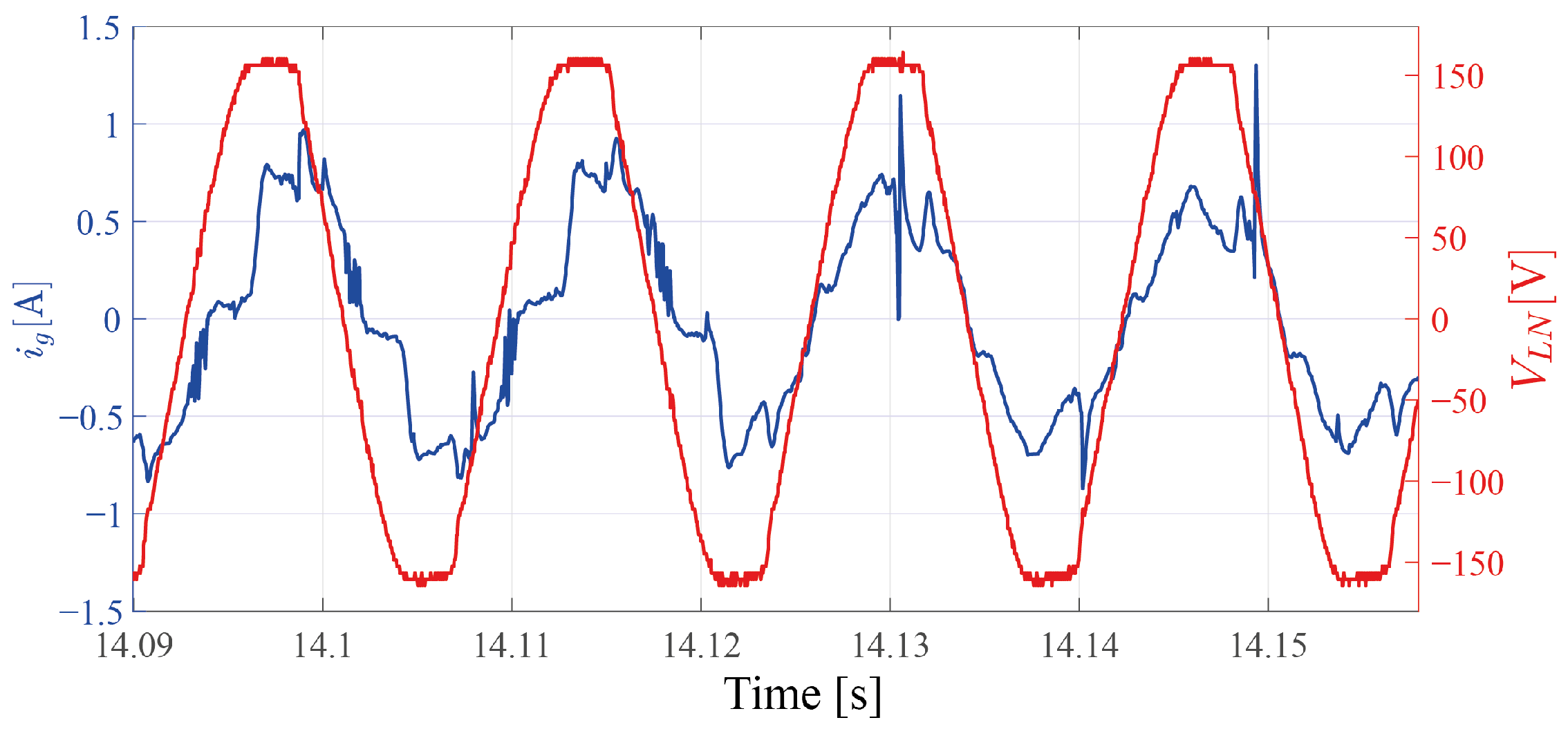
3.2. Experimental Results

As in the simulation results, different case studies are proposed in order to evaluate the behavior of the microinverter in both the DC-DC stage and the DC-AC stage. The data were measured with a SIGLENT SHS1062 oscilloscope and a sampling frequency of 25 kHz.

For the DC-DC stage, the voltage and current values of the solar panel were measured at an irradiance of approximately 263 W/m${}^2$ so that the ideal power was 79 W. In Figure 37, the current and voltage of the panel with filtered and measured data can be observed. In Figure 38, the input power is shown, where it can be deduced that the MPPT algorithm, in conjunction with the 2P2Z control, managed to obtain the maximum power from the panel. However, oscillations occurred, mainly due to high-frequency noise, so they were eliminated with the designed digital filters.

In addition to having an on-grid operating mode, the microinverter can be configured for an off-grid mode. Figure 39 shows the current $i_g$, the output voltage, and the $TH{D}_i=7.63\%$ obtained with this configuration, which were in a range close to that suggested by the IEEE 1547 standard [31]. This case study was carried out to verify the control algorithm, PWM configuration, and microinverter operation before synchronizing with the grid.

After verifying the proper functioning of the microinverter in the off-grid mode, the synchronization stage with the grid and the active and reactive power control were implemented to obtain the results for the DC-AC stage. In Figure 40, the PI voltage control response, which was activated at 1.2 s, is shown. It is evidenced that the DC bus voltage managed to follow the 270 V reference without steady-state error and with a settling time of approximately 0.5 s.

Then, $P_{ref}$ was set to be equal to $P_{\mathit{max}}$, and $Q_{\mathit{ref}}$ was defined with the values of 0, 20, 40, −20, and −40 VAr to analyze the active and reactive power control. Figure 41 shows that the P and Q control supplied capacitive and inductive reactive power according to the defined reference.In addition, the injected active power is presented.

When $Q_{\mathit{ref}}$ changed from 40 to 0 VAR, the injected current of the microinverter $i_g$ and the grid voltage $V_{LN}$ were compared (Figure 42), and a difference in the phase shift between the two waves of approximately 35 ${}^{°}$ a 0${}^{°}$ was shown.

Similarly, the reactive power reference values for the microinverter must be established with a minimum power factor of ±0.85 or ±53% of the total reactive power to function correctly and guarantee the integrity of its components.

A scenario with a 100 W incandescent light bulb was proposed to analyze the interaction of the microinverter with the grid (Figure 43). In the beginning, the microinverter control was off and, after 4.7 s, it was activated. The microinverter managed to partially compensate the active power consumption of the load when the control system was on.

From the previous case studies, some indicators were calculated to evaluate the performance of the microinverter. The combined efficiency of the DC-DC stage and the DC-AC stage was, on average, $88\%$, and the maximum was $91\%$, which was similar to that found in [19]. In addition, the total harmonic distortion was calculated (Figure 44); $TH{D}_v=9.4\%$ and $TH{D}_i=24.9\%$ were obtained, which are values that were outside the range established by the IEEE 1547 standard [31]. However, these effects may be associated with distortions in the data collected because a THD of $7.6\%$ was found in the off-grid configuration.

4. Conclusions

This research presented the design and implementation of an on-grid microinverter control technique for managing active and reactive power based on a dq transformation. The simulated model allowed us to approach the real behavior of the system, and good performance was obtained for the control techniques. In the DC-DC stage, the maximum power point of the panel was monitored with the generation of the current reference, which was given by the incremental conductance MPPT algorithm and regulated by a 2P2Z control. This algorithm is robust against continuous changes in irradiance, as it quickly follows the ideal power and it always operates at a point close to the MPP. In addition, the 2P2Z control allowed the panel current to follow the reference without steady-state error and low oscillations, results that were evidenced in the simulations and experimentally.

Furthermore, In the DC-AC stage, an anti-windup PI controller was implemented for the DC bus voltage; it followed the desired reference to regulate the active power supplied by the microinverter. Furthermore, a second-order generalized integrator (SOGI)-based phase-locked loop (PLL) was employed to calculate the P and Q control. In addition, a 3P3Z current controller was applied, which followed the reference given by the P and Q control. Moreover, a feedback linearization technique was implemented to compensate for disturbances caused by the voltage of the grid in the 3P3Z control.

Moreover, the P and Q control implemented in the TI solar microinverter and simulations delivered the maximum active power. It supplied reactive power according to a defined reference and within the established limits. In addition, the integration of the microinverter into a microgrid could be performed due to the possibility of changing the reference values of the DC bus voltage and P and Q powers supplied by a secondary control.

This research demonstrated that it is possible to simulate control techniques that behave similarly to those of real equipment to ensure proper operation during implementation. Additionally, it was possible to demonstrate the viability of active and reactive power control techniques using a low-cost commercial microinverter. Finally, by implementing an active and reactive power control technique in a low-power microinverter, these controls can be used in small microgrids to maintain power quality.

In future work, the LCL filter and the structure of the dual-buck inverter can be improved in order to obtain lower harmonic distortion levels in the output current of the microinverter. In addition, the PWM control can be improved to reduce oscillations or distortions around the zero-crossing area. Additionally, it is possible to implement other active and reactive power control techniques and integrate the microinverter into a secondary control for a microgrid.

References

1. Meng, L.; Savaghebi, M.; Andrade, F.; Vasquez, J.C.; Guerrero, J.M.; Graells, M. Microgrid central controller development and hierarchical control implementation in the intelligent microgrid lab of Aalborg University. In Proceedings of the 2015 IEEE Applied Power Electronics Conference and Exposition (APEC), Charlotte, NC, USA, 15–19 March 2015; pp. 2585–2592. [Google Scholar] [CrossRef] [Green Version]
2. Ortega, R.; García, V.H.; García-García, A.L.; Rodriguez, J.J.; Vásquez, V.; Sosa-Savedra, J.C. Modeling and Application of Controllers for a Photovoltaic Inverter for Operation in a Microgrid. Sustainability 2021, 13, 5115. [Google Scholar] [CrossRef]
3. Caporal, M.; Magdaleno, J.J.R.; Cruz Vega, I.; Caporal, R.M. Improved grid-photovoltaic system based on variable-step MPPT, predictive control, and active/reactive control. IEEE Lat. Am. Trans. 2017, 15, 2064–2070. [Google Scholar] [CrossRef]
4. Abadlia, I.; Bahi, T.; Lekhchine, S.; Bouzeria, H. Active and reactive power neurocontroller for grid-connected photovoltaic generation system. J. Electr. Syst. 2016, 12, 146–157. [Google Scholar]
5. Talha, M.; Raihan, S.; Rahim, N.A. PV inverter with decoupled active and reactive power control to mitigate grid faults. Renew. Energy 2020, 162, 877–892. [Google Scholar] [CrossRef]
6. Zeb, K.; Nazir, M.S.; Ahmad, I.; Uddin, W.; Kim, H.J. Control of Transformerless Inverter-Based Two-Stage Grid-Connected Photovoltaic System Using Adaptive-PI and Adaptive Sliding Mode Controllers. Energies 2021, 14, 2546. [Google Scholar] [CrossRef]
7. Ishfaq, M.; Uddin, W.; Zeb, K.; Islam, S.U.; Hussain, S.; Khan, I.; Kim, H.J. Active and Reactive Power Control of Modular Multilevel Converter Using Sliding Mode Controller. In Proceedings of the 2019 2nd International Conference on Computing, Mathematics and Engineering Technologies (iCoMET), Sukkur, Pakistan, 30–31 January 2019; pp. 1–5. [Google Scholar] [CrossRef]
8. El Aamri, F.; Maker, H.; Mouhsen, A.; Harmouchi, M. A new strategy to control the active and reactive power for single phase grid-connected PV inverter. In Proceedings of the 2015 3rd International Renewable and Sustainable Energy Conference (IRSEC), Marrakech, Morocco, 10–13 December 2015; pp. 1–6. [Google Scholar] [CrossRef]
9. Babaie, M.; Mehrasa, M.; Sharifzadeh, M.; Melis, G.; Al-Haddad, K. DQ-Based Radial Basis Function Controller for Single-Phase PEC9 Inverter. In Proceedings of the 2020 IEEE 29th International Symposium on Industrial Electronics (ISIE), Delft, The Netherlands, 17–19 June 2020; pp. 701–706. [Google Scholar] [CrossRef]
10. Andrade, I.; Pena, R.; Blasco-Gimenez, R.; Riedemann, J.; Jara, W.; Pesce, C. An Active/Reactive Power Control Strategy for Renewable Generation Systems. Electronics 2021, 10, 1061. [Google Scholar] [CrossRef]
11. Toub, M.; Bijaieh, M.M.; Weaver, W.W.; Robinett, R.D.; Maaroufi, M.; Aniba, G. Droop Control in DQ Coordinates for Fixed Frequency Inverter-Based AC Microgrids. Electronics 2019, 8, 1168. [Google Scholar] [CrossRef] [Green Version]
12. Bolaños-Navarrete, M.A.; Osorio, G.; Bastidas-Rodriguez, J.D.; Revelo-Fuelagan, E.J. Computational Model of a Two-stage Microinverter With Flyback Active Clamp and Dual Buck. In Proceedings of the 2019 IEEE 4th Colombian Conference on Automatic Control (CCAC), Medellin, Colombia, 15–18 October 2019; pp. 1–6. [Google Scholar] [CrossRef]
13. Mo, Q.; Chen, M.; Zhang, Z.; Zhang, Y.; Qian, Z. Digitally controlled active clamp interleaved flyback converters for improving efficiency in photovoltaic grid-connected micro-inverter. In Proceedings of the 2012 Twenty-Seventh Annual IEEE Applied Power Electronics Conference and Exposition (APEC), Orlando, FL, USA, 5–9 February 2012; pp. 555–562. [Google Scholar] [CrossRef]
14. Khan, A.A.; Cha, H.; Lai, J. Cascaded Dual-Buck Inverter With Reduced Number of Inductors. IEEE Trans. Power Electron. 2018, 33, 2847–2856. [Google Scholar] [CrossRef]
15. Cho, M.G.; Lee, S.H.; Lee, H.S.; Choi, Y.G.; Kang, B. Circuit Structure and Control Method to Reduce Size and Harmonic Distortion of Interleaved Dual Buck Inverter. Energies 2020, 13, 1531. [Google Scholar] [CrossRef] [Green Version]
16. Vera-Dávila, A.G.; Delgado-Ariza, J.C.; Sepúlveda-Mora, S.B. Validación del modelo matemático de un panel solar empleando la herramienta Simulink de Matlab. Rev. Investig. Desarro. Innov. 2018, 8, 343–356. [Google Scholar] [CrossRef] [Green Version]
17. Mahmud, M.A.; Pota, H.R.; Hossain, M.J. Nonlinear Current Control Scheme for a Single-Phase Grid-Connected Photovoltaic System. IEEE Trans. Sustain. Energy 2014, 5, 218–227. [Google Scholar] [CrossRef]
18. Kazimierczuk, M.K. Pulse-Width Modulated DC-DC Power Converters; John Wiley & Sons: Hoboken, NJ, USA, 2015; pp. 195–241. [Google Scholar]
19. Bhardwaj, M.; Choudhury, S. Digitally Controlled Solar Micro Inverter Design using C2000 Piccolo Microcontroller; Texas Instruments Inc.: Dallas, TX, USA, 2017. [Google Scholar]
20. Raj, A.S.; Siddeshwar, A.M.; Guruswamy, K.P.; Maheshan, C.M.; Vijay Sanekere, C. Modelling of flyback converter using state space averaging technique. In Proceedings of the 2015 IEEE International Conference on Electronics, Computing and Communication Technologies (CONECCT), Bangalore, India, 10–11 July 2015; pp. 1–5. [Google Scholar] [CrossRef] [Green Version]
21. González-Castaño, C.; Lorente-Leyva, L.L.; Muñoz, J.; Restrepo, C.; Peluffo-Ordóñez, D.H. An MPPT Strategy Based on a Surface-Based Polynomial Fitting for Solar Photovoltaic Systems Using Real-Time Hardware. Electronics 2021, 10, 206. [Google Scholar] [CrossRef]
22. Alzahrani, A. A Fast and Accurate Maximum Power Point Tracking Approach Based on Neural Network Assisted Fractional Open-Circuit Voltage. Electronics 2020, 9, 2206. [Google Scholar] [CrossRef]
23. Jalali Zand, S.; Hsia, K.H.; Eskandarian, N.; Mobayen, S. Improvement of Self-Predictive Incremental Conductance Algorithm with the Ability to Detect Dynamic Conditions. Energies 2021, 14, 1234. [Google Scholar] [CrossRef]
24. Islam, H.; Mekhilef, S.; Shah, N.M.; Soon, T.K.; Wahyudie, A.; Ahmed, M. Improved Proportional-Integral Coordinated MPPT Controller with Fast Tracking Speed for Grid-Tied PV Systems under Partially Shaded Conditions. Sustainability 2021, 13, 830. [Google Scholar] [CrossRef]
25. Seguel, J.L.; Seleme, S.I. Robust Digital Control Strategy Based on Fuzzy Logic for a Solar Charger of VRLA Batteries. Energies 2021, 14, 1001. [Google Scholar] [CrossRef]
26. Bakkar, M.; Aboelhassan, A.; Abdelgeliel, M.; Galea, M. PV Systems Control Using Fuzzy Logic Controller Employing Dynamic Safety Margin under Normal and Partial Shading Conditions. Energies 2021, 14, 841. [Google Scholar] [CrossRef]
27. Kumar Chaurasia, M.; Gidwani, L. Analysis of PV module with buck-boost and zeta converters with incremental conductance maximum power point tracking method. In Proceedings of the 2017 International Conference On Smart Technologies For Smart Nation (SmartTechCon), Bengaluru, India, 17–19 August 2017; pp. 1591–1596. [Google Scholar] [CrossRef]
28. Ikken, N.; Bouknadel, A.; Haddou, A.; Tariba, N.; El omari, H.; El omari, H. PLL Synchronization Method Based on Second-Order Generalized Integrator for Single Phase Grid Connected Inverters Systems during Grid Abnormalities. In Proceedings of the 2019 International Conference on Wireless Technologies, Embedded and Intelligent Systems (WITS), Fez, Morocco, 3–4 April 2019; pp. 1–5. [Google Scholar] [CrossRef]
29. Suyata, T.; Po-Ngam, S. Simplified active power and reactive power control with MPPT for three-phase grid-connected photovoltaic inverters. In Proceedings of the 2014 11th International Conference on Electrical Engineering/Electronics, Computer, Telecommunications and Information Technology (ECTI-CON), Nakhon Ratchasima, Thailand, 14–17 May 2014; pp. 1–4. [Google Scholar] [CrossRef]
30. Gi-Power New Energy. Polycrystalline Module Models. GP-150P-36; Gi-Power New Energy: Dongguan, China, 2017. [Google Scholar]
31. IEEE. IEEE Application Guide for IEEE Std 1547(TM), IEEE Standard for Interconnecting Distributed Resources with Electric Power Systems. IEEE Std 1547.2-2008; IEEE: Piscataway, NJ, USA, 2009; pp. 1–217. [Google Scholar] [CrossRef]
Figure 1. General diagram of the system.
Applsci 11 04765 g001
Figure 2. Equivalent circuit of the solar panel for N s photovoltaic cells in series and N p modules in parallel [17].
Applsci 11 04765 g002
Figure 3. Active clamp flyback converter, where Q a c operates in a mode complementary to the main MOSFET Q 1 [19].
Applsci 11 04765 g003
Figure 4. DC-AC circuit of the dual-buck inverter. First buck converter: Q 6 , Q 3 , D 1 , and L 4 . Second buck converter: Q 5 , Q 4 , D 2 , and L 3 [19].
Applsci 11 04765 g004
Figure 5. Behavior of the PWMs for each half cycle V L N .
Applsci 11 04765 g005
Figure 6. LCL inverter filter.
Applsci 11 04765 g006
Figure 7. Characteristic curve of a solar panel with irradiance values from 100 to 1000 W/m 2 .
Applsci 11 04765 g007
Figure 8. DC-DC stage control loop; the current-based incremental conductance MPPT is regulated by a 2P2Z controller.
Applsci 11 04765 g008
Figure 9. Flow diagram of the current-based incremental conductance algorithm.
Applsci 11 04765 g009
Figure 10. 2P2Z controller with a double saturator.
Applsci 11 04765 g010
Figure 11. Discrete Fourier transform of the solar panel current.
Applsci 11 04765 g011
Figure 12. Control loop of the DC-AC stage.
Applsci 11 04765 g012
Figure 13. Second-order generalized integrator (SOGI)-based phase-locked loop (PLL) [19].
Applsci 11 04765 g013
Figure 14. Diagram of the second-order generalized integrator (SOGI).
Applsci 11 04765 g014
Figure 15. Reference frames of the Park transformation.
Applsci 11 04765 g015
Figure 16. Current-control loop with feedback linearization.
Applsci 11 04765 g016
Figure 17. TI solar microinverter.
Applsci 11 04765 g017
Figure 18. Input and output diagram of the F28035 Piccolo controlCARD used to control the DC-DC and DC-AC stages of the microinverter.
Applsci 11 04765 g018
Figure 19. Processes of the program and tasks in the CPU (main core) and CLA (secondary core).
Applsci 11 04765 g019
Figure 20. Overvoltage and overcurrent protection task.
Applsci 11 04765 g020
Figure 21. Serial communication task.
Applsci 11 04765 g021
Figure 22. Current-based incremental conductance MPPT task.
Applsci 11 04765 g022
Figure 23. Structure of the inverter task.
Applsci 11 04765 g023
Figure 24. Reference used to model the behavior of irradiance during the day.
Applsci 11 04765 g024
Figure 25. Reference, measured, and filtered signals for the current of the solar panel.
Applsci 11 04765 g025
Figure 26. Tracking the maximum power of the solar panel.
Applsci 11 04765 g026
Figure 27. Currents of the main inductor and output of the LCL filter.
Applsci 11 04765 g027
Figure 28. Measured and filtered voltage in the DC bus.
Applsci 11 04765 g028
Figure 29. Active power delivered by the microinverter, active power supplied by the electrical grid, and active power consumed by the load. Reference value: V ref = 250 V.
Applsci 11 04765 g029
Figure 30. Reactive power injected by the microinverter and its reference, reactive power from the grid, and the reactive power demanded by the load. Reference value: V ref = 250 V.
Applsci 11 04765 g030
Figure 31. Current and voltage injected into the grid during the change in Q ref from 0 to 165 VAR.
Applsci 11 04765 g031
Figure 32. FFT analysis; output current THD of the microinverter.
Applsci 11 04765 g032
Figure 33. Power factor and efficiency during the changes in Q ref .
Applsci 11 04765 g033
Figure 34. Possible working range of the microinverter based on reactive power.
Applsci 11 04765 g034
Figure 35. Interaction of the microinverter with the grid when Q ref = Q load . Reference value: V ref = 250 V.
Applsci 11 04765 g035
Figure 36. Increase in V bus in order to regulate the active power. Reference value: Q ref = 0 VAR.
Applsci 11 04765 g036
Figure 37. Current and voltage of the solar panel when the irradiance was 263 W/m 2 .
Applsci 11 04765 g037
Figure 38. Power obtained from the solar panel.
Applsci 11 04765 g038
Figure 39. Output current and voltage of the microinverter configured in the off-grid mode.
Applsci 11 04765 g039
Figure 40. Voltage of the DC bus. The microinverter control was activated at 1.2 s. V ref = 270 V.
Applsci 11 04765 g040
Figure 41. Active and reactive power supplied by the microinverter during the changes in Q ref . Reference value: V ref = 270 V.
Applsci 11 04765 g041
Figure 42. Current injected by the microinverter and voltage of the grid during variation in Q ref from 40 to 0 VAR.
Applsci 11 04765 g042
Figure 43. Interaction of the microinverter with the grid and with a load of 100 W. Reference values: V ref = 270 V.
Applsci 11 04765 g043
Figure 44. FFT analysis, current THD, and output voltage.
Applsci 11 04765 g044