Abstract
Tomographic reconstruction allows for the recovery of 3D information from 2D projection data. This commonly requires a full angular scan of the specimen. Angular restrictions that exist, especially in technical processes, result in reconstruction artifacts and unknown systematic measurement errors. We investigate the use of neural networks for extrapolating the missing projection data from holographic sound pressure measurements. A bias flow liner was studied for active sound dampening in aviation. We employed a dense U-Net trained on synthetic data and compared reconstructions of simulated and measured data with and without extrapolation. In both cases, the neural network based approach decreases the mean and maximum measurement deviations by a factor of two. These findings can enable quantitative measurements in other applications suffering from limited angular access as well.
1. Introduction
Tomographic reconstruction of projection fields has been used in many areas for decades. It is an established technique for 3D imaging and measurement in medicine [1,2,3,4,5], geoscience [6], for studying combustion [7] or materials science [8]. Another important field is in acoustic research, where it is becoming increasingly important with modern technology to make complex acoustic phenomena visible for the first time [9].
In this field, especially the noninvasive volumetric measurement of sound pressure fields, there is a suitable application for tomographic reconstructions [10]. For investigations of local phenomena, for instance in sound dampers such as the bias-flow-liners in aircraft turbines, it is necessary to perform measurements within a flow channel in order to mimic the conditions of real applications [11,12]. However, in a flow channel, it is not possible to measure parallel to the flow direction without disturbing the flow. This results in a limitation of the angular scan range available for the measurement. Often, the angular scan range is limited from at ideal conditions to about due to technical facilities [13].
Tomographic reconstruction algorithms such as filtered back projection require a measurement from different scan angle positions in the range of [9]. Limitations of the angular scanning range result in artifacts such as diagonal lines in the local reconstruction field and disappearance of sharp edges outside the scan angle range occurs [1,2,3,14,15]. Furthermore, an unknown systematic measurement error occurs, i.e., the absolute values of the reconstruction are strongly distorted [16,17]. To improve the reconstruction result, additional prior knowledge about the measurement object must be integrated into the reconstruction process. This could be iterative approaches such as algebraic reconstruction technique [18] or total variation [18]. They need a lot of computing power but can use estimations as initial value for the reconstruction. Errors in initial estimation can distort the complete reconstruction.
The hypothesis in this publication is that neural networks can be used to extrapolate data from missing scan angles to significantly improve reconstruction results. This enables the use of standard algorithms for the tomographic reconstruction. There are several existing deep learning based approaches employing neural networks to directly reconstruct local data. They replace the established standard reconstruction methods, such as filtered back projection, and achieve good results, for instance with sparse angle tomography [19,20,21,22,23]. Synthetic data are used for training and validation. Finally, reconstruction improvements of real limited angle sound pressure measurements are presented.
2. State-of-the-Art
2.1. Sound Pressure Measurements
A standard method for quantitative sound pressure measurements is the detection by condenser microphones [24]. This allows for point-like measurement. The extension to a measurement field of one, two or three dimensions is possible with a matrix arrangement of microphones. By using beam forming, a two-dimensional arrangement of microphones is sufficient for a three-dimensional reconstruction [25]. However, measurements with microphones are invasive and distort the sound pressure field [26]. Furthermore, microphones typically feature diameters of several millimeters and have a direction characteristic, limiting the spatial resolution to several millimeters and distorting measurements based on relative sound source position [27]. An alternative, noninvasive measurement principle is the measurement of the transfer function between two microphones. This function then describes the acoustic behavior between the two measurement points but offers no spatial resolution [28].
A noninvasive approach based on laser interferometric vibrometry (LIV) can be used for sound pressure measurement. The LIV measures the integral, sound-induced refractive index variation along the optical path [29]. If the measurement is also performed from different angles, the reconstruction of the local sound field for a point in the measurement volume can be calculated by tomographic reconstruction algorithms. This principle can be extended to a measurement plane or volume by using a camera as detector. At high-speed camera-based laser interferometric vibrometers (CLIV), each camera pixel performs a simultaneous line integral measurement [30].
2.2. CLIV
When a laser beam passes through an acoustically active volume, the phase of the light wave changes as a function of the sound wave due to the sound-induced change of the refractive index. This is called the optoacoustic effect [9].
Consider a simple LIV set-up, a plane wave sound source and a photo detector. The laser beam travels through a known constant distance l. Let the plane sound wave excite the medium along l. Over time the sound wave creates areas of higher density and areas of lower density in dependence of the current spatial and temporal sound pressure wave propagation. This oscillation is given by the frequency and amplitude of the sound wave. The changes in the light intensity are detected as a phase shift [9]. The intensity signal of the laser light can be described as:
depending on the modulation depth V and the phase shift . The intensity signal oscillates with the instant frequency
where represents the carrier frequency and the frequency shift. A fluctuation of the sound field results in a fluctuation of the frequency shift
in dependency of the laser wavelength and the time derivative of the optical path length
i.e., the line integral over the refractive index n along the laser beam [10]. The Gladstone–Dale theorem [30] provides the mathematical link between the refractive index and the density of the medium:
with the material dependent Gladstone–Dale constant G. Using Equations (2)–(5) and the assumption of an adiabatic change of state, the one-dimensional acousto-optical relationship between the instant frequency and the time derivative of the sound pressure along the optical path can be established:
where is the adiabatic exponent, and are the refractive index and the pressure under reference conditions, respectively. This equation is valid for a projection line in the measurement volume. Thus, the integral sound pressure can be estimated from the detected intensity signals instant frequency . In order to detect negative and positive frequency shifts, i.e., heterodyne detection, and to define a measurement range for , the laser light has to be modulated with a carrier frequency [7]. This can be achieved by using an acousto-optical modulator (AOM). Finally, the photo detector has to be fast enough to capture the high-frequency fluctuations .
The extension of this technique is the matrix measurement of many projections with a camera. Figure 1 shows the camera-based laser interferometer. This enables a three-dimensional tomographic measurement of local sound pressure fields with a spatial resolution of 31.5 μm at a sampling rate of 120 kHz.
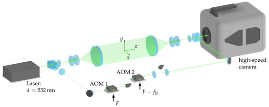
Figure 1.
Measurement principle of the heterodyne Mach–Zehnder interferometer. Laser: nm, solid state laser; camera: 64 × 1024 Pixel, : 30 kHz, field of view: 2 × 30 mm, frame rate: 120 kHz. Taken from [7].
2.3. Tomographic Reconstruction
The optical measurement of sound pressure can only be done in projection. This means that a two-dimensional tomographic reconstruction must be performed. The solution of this inverse problem can be done using the filtered back projection.
The tomographic reconstruction is performed as follows: Let the measurement of a projection be a vector to in a transformed plane from an angular perspective of the rotation angle as shown in Figure 2. Using a total number of scan lines and angular scans these vectors give the sinogram with dimensions (see Figure 3).
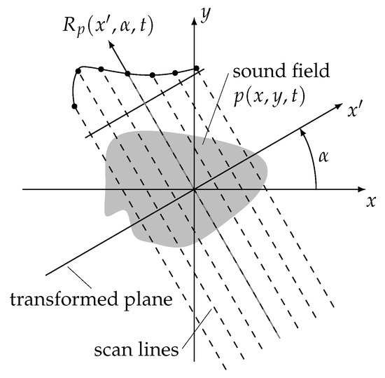
Figure 2.
Principle of the Radon transformation.
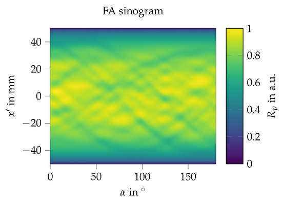
Figure 3.
Full angle (FA) sinogram in angular range .
Mathematically, a sinogram is the forward operation of the Radon transformation. Thus, a solution of the inverse problem by applying the inverse Radon transformation is needed for the reconstruction of the sound field
with the filter function . Due to the integral operation of the inverse transformation, low-frequency components are weighted higher than high-frequency components. With the filter function this weighting error can be corrected during the reconstruction. This leads to a sharper image and ensures an absolute value reconstruction [9]. Different types of filters can be considered as a filter function. For example, there is the Ram–Lak filter with a linear increase of the amplitude over the frequency, the well-known Hamming filter or the Hanning filter [31]. While the Ram–Lak filter is sensitive to noise, it has provided the best absolute value reconstruction results, which was tested on simulated data. Thus, the Ram–Lak filter will be used for all reconstructions on simulated and measured data in the following investigations for a fair comparison.
There are prerequisites in the measurement setup to reconstruct a local field. For example, the field to be measured must be scanned from different directions in an angular range of and high angular resolution [10]. The angle resolution depends on the crucial spatial resolution of the local field. Sparse angular sampling can result in aliasing [10]. Furthermore, a stationary and spatially closed field is required [9]. If these prerequisites are violated, strong artifact formation and additional information loss of the local absolute values will occur. A high angular limitation results in high artifact formation also known as missing cone artifacts [32]. This is caused by an incorrect frequency weighting, as well as the systematic reconstruction deviation of the absolute amplitude, caused by numeric instabilities, compared to the model field [17].
2.4. Deep Learning
Neural networks differ from analytical approaches in one fundamental aspect. Analytical approaches use a deterministic mathematical model to represent the transformation equation from input to output. On the other hand, neural networks are modeled by an adaptive mathematical equation. This equation consists of an input vector X, a weight vector W and a bias b [16]:
Equation (8) represents a neuron k, which exhibits a nonlinear activation function f. This again produces a nonlinear transformation of the input signal. Weights are parameters updated by error propagation, also known as backpropagation. Neurons are usually grouped into layers, which can be distinguished into input, hidden and output layers. The connection model between layers can vary. So, comprehensible task processing can be achieved. The most common layer topologies are perceptron layers as well as convolutional layers. This last type is particularly efficient for tasks regarding image processing [19,33,34]. The type of neural network is determined by its architecture. This refers to the size, type and connection model that exists between the layers. The implementation of convolutional layers in neural networks has become a crucial factor for image processing tasks in recent years [19,35]. An example of this, is the Unet in Figure 4, top. Later, the Dense Unet has shown improvement (Figure 4, overall) by replacing convolutional layers with denseblocks [19]. Here, a denseblock consists of a set of convolutional layers concatenated using a skip-layer strategy (see Figure 4, bottom). Similar to a convolutional layer, dense blocks have their own hyperparameters, such as the growth rate k and the number of repetitions l. The growth rate k refers to the feature layers that are calculated from the previous step. Then, l indicates how many times k feature layers will be concatenated.
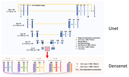
Figure 4.
Dense Unet architecture (top) used for limited angle tomographic image reconstruction. Example of denseblock structure (bottom), with hyperparameters k = 8 and l = 4.
With the use of dense blocks in every convolutional step, there are more connections between every neuron in the step. Thus, the overfitting can be reduced [36]. The disadvantage is a larger number of hidden layers, which requires more computing power and increases the training time.
3. Experimental Setup and Methodology
3.1. Experimental Setup and Measurement Execution
The aim was to enable a complete reconstruction of the local sound pressure under a limited incomplete angle. For this purpose, a full angle projection measurement of the sound field was performed with the CLIV system proposed in [9] as a reference. The sound field to be investigated was limited by a translucent PMMA cylinder of 100 mm diameter to allow a angular scan range of and shield the reference beam of the interferometer from the propagating sound wave in the measurement object. An approximately plane sound wave was generated by a speaker mounted to the top end of the tube. Thus, the sound wave propagates perpendicular to a hexagonal array of 169 Helmholtz resonators at the bottom of the cylinder (see Figure 5). Each Helmholtz resonator is cylindrical, has a resonator volume of 1.41 cm and a hole aperture of 2 mm diameter (see Figure 6). This results in a resonator frequency of 1479 Hz. The measurement of the local sound field was performed at the resonator frequency. The maximum effective lateral range of the CLIV system is 25 mm with a spatial resolution of 31.5 μm. In order to perform a measurement of the entire cylinder, the measurement was divided into seven, 2 cm wide lateral areas, which were stitched in post-processing.
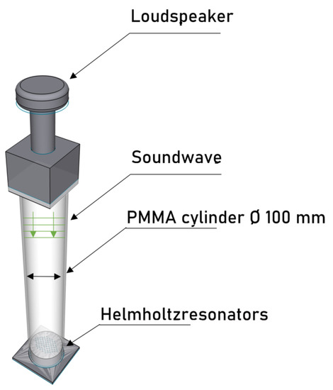
Figure 5.
Acoustic measurement setup for generating a local sound field with optical access.
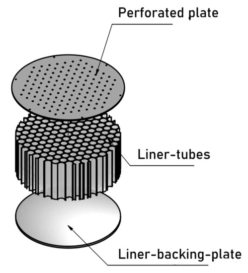
Figure 6.
Liner model used for measurements, providing 169 Helmholtz resonators.
The measurement procedure starts with setting the lateral position. After that follows the measurement of each scan angle with a resolution of in a angular scan range of . When a scan is completed, the next lateral position is scanned.
The measuring time per single angle scan is 1s. In addition, there is a camera hardware-related memory cycle of approx. 2 min, which is decisive for the total measurement time per scan point. The measurement volume is located 31.5 μm above the resonator surface. This allows for the largest possible local sound pressure changes and avoids reflections from the resonator surface that affect the measurement result. The measuring system is capable of recording a pixel area of 64 pixels in height with the necessary frequency. However, only a reduced height of 16 px was used in order to speed up the measuring process.
3.2. Methodology
To investigate the performance of the neural network, a projection measurement of the sound field above the hexagonal measurement object was performed using CLIV. The reconstruction of the fully measured angular scan range will later serve as a validation object.
The goal is to provide a complete reconstruction of the local sound pressure under constrained angle. Therefore, an additional computational step was introduced with the neural network to extrapolate the missing information. The complete process is described in Figure 7. For validation and comparison of the reconstruction of the sound pressure data, angular information was removed from the full measurement to create a constrained angle sinogram. These data were fed into the neural network. Due to the complex structure of the network, there are computational limitations. The pixel resolution of the projection data at input as well as output is limited to 256 angle measurements at 1024 individual projection lines per lateral plane. Hence, the remaining spatial resolution after the extrapolation process is 97.6 μm. Only the missing angle information is reconstructed by the neural network. Using the original angle constrained data, the complete sinogram can be assembled. However, the extrapolated part of the sinogram has a different angular resolution than the measured part. This means that resampling of the full sinogram must be performed.
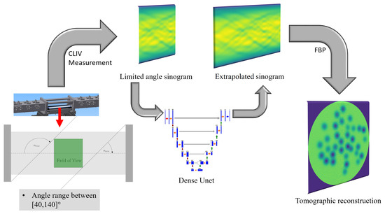
Figure 7.
Flow chart for processing limited angle tomography: Projection data are recorded holograhically with limited angle (LA) access and assembled into a sinogram. The limited angle sinogram is fed into a pretrained dense Unet and the missing projection data are extrapolated. Filtered back projection is then used to calculate the local field.
3.3. Neuronal Network Training
In order to enable extrapolation, the neural network must be trained. For this purpose, a training data set was created from 60,000 synthetically generated sound pressure fields. These sound pressure fields were modeled after a tomographic measurement of a Kundt’s tube at an angular access of (see Figure 5). The measured model is a hexagonal array of Helmholtz resonators with a circular resonator aperture. The size of the resonator holes (; ), the number of resonators , the distance between the resonators (; ), the amplitude above the resonators () and the orientation of the start scan angle () were varied. This is superimposed by a static sound pressure throughout the cylinder (offset). In the region of the apertures there is a Gaussian reduction of the sound pressure. The parameter range of the randomly varied quantities is listed in Table 1. By randomly choosing the above parameters, an asymmetric pattern is guaranteed for each image. Only in case of such asymmetric modeling an angular scan of is necessary. Extrapolation of the neural network by repetition and mirroring of already existing areas of the input data can thus be excluded.

Table 1.
Parameters used for sound field generation.
For training, 80% of the data set was used. The remaining data were used as a validation data set. A total of 24 epochs were trained to converge the loss function to a acceptable remaining loss and thus, the extrapolation results can not be substantially improved. Additionally, the problem of overfitting is minimal. The overfitting and thus the difference of the loss function between training data set and validation data set after 24 epochs was less than 0.3%.
The training results are shown in Figure 8. Good reconstruction results have been obtained. Mean squared error (MSE) and structural similarity (SSIM) [37] were used as comparison values. The MSE is calculated according to the following formula:
where the coordinates x and y are the lateral and axial positions of a reconstructed plane.
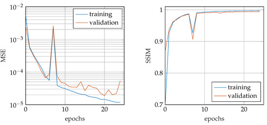
Figure 8.
Visualization of training process with 60,000 data sets (48,000 training data set; 24,000 validation data set) over 24 epochs. As validation parameters mean squared error (MSE) and structural similarity (SSIM) are shown.
Starting with the 2nd epoch, an MSE lower than 0.1% is reached. In epoch 7, there is a sudden increase of the error to 0.27% in the validation data set. This can be explained by the NADAM optimization algorithm used. The algorithm does not run into a local minimum, but tries to reach the global minimum. Thus, due to abrupt changes in the optimized weights, the error may increase abruptly [38]. After 24 epochs, an error of the MSE of less than 0.005% was reached. The impact of an overfitting effect is negligible after 24 epochs. The same result can be seen for SSIM, which reaches a value of 99.4% after 24 epochs of training. The training took 11 h on a high performance workstation with an Nvidia TITAN RTX GPU. After training the extrapolation process took in summary 35 s for one extrapolation process. This time is mainly limited by the loading and saving process of the data.
4. Results
4.1. Synthetic Data
A synthetic sound pressure field was generated according to the parameters presented in Table 1 (2. line). The first row of Figure 9 shows the sinograms with full scanning angle (a), limited scanning angle (LA) (b) and the neuronal network based extrapolation (c). The second row shows corresponding local data computed by filtered back projection (d–f). The bottom row describes the relative error referred to the full angle filtered back projection tomographic reconstruction. The local error for limited angle and neural network reconstruction are depicted in (h,i). Boxplots at (g) show the corresponding error distribution.
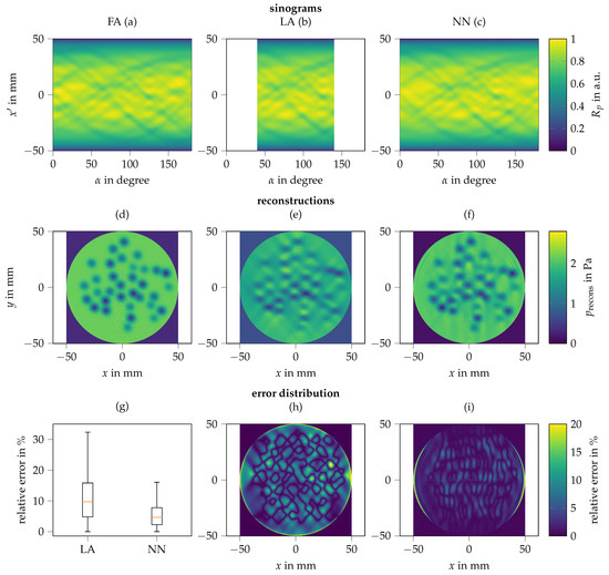
Figure 9.
Synthetic sound pressure field reconstruction: (a) full angle (FA) sinogram; (b) limited angle (LA) sinogram; (c) neural network (NN) extrapolated sinogram; (d) full angle filtered back projection tomographic reconstruction; (e) limited angle filtered back projection tomographic reconstruction; (f) neural network extrapolated filtered back projection tomographic reconstruction; (g) error distribution of local reconstructions compared to full angle reconstruction; (h) local error of limited angle reconstruction compared to full angle reconstruction; (i) local error of neural network reconstruction compared to full angle reconstruction.
The modeled constant sound pressure field in the cylinder (Figure 9i) results in a quadratic function in the sinogram over the projection axis. In the angular axis, the function is constant. Each hole produces a reduction in the total amplitude on each measurement in the angular scan range. If several resonators are in succession in the direction of projection, the reduction in amplitude is summed. The hole position has a sinusoidal curve over the scanned angle axis. These correlations were learned without the possibility of mirroring or repeating certain parts of the already given range by training the neural network.
It can be seen that a reconstruction using filtered back projection of the measurement data with full angular scan range leads to an artifact-free reconstruction result, only higher noise emissions are visible. On the contrary, when reconstructing with a limited angular scan range, clear artifacts can be seen. Individual resonators have an elliptical shape and become blurred. This leads to an inseparability of individual resonators if they are close to each other. Furthermore, an incorrect absolute value reconstruction occurs, which deviates both downwards and upwards. Locally, especially between neighboring resonators, excessive sound pressure values are reconstructed and the values within a hole are calculated as too low. The sinogram extrapolated by means of neural network shows a considerable qualitative improvement in the reconstruction. The resonators regain their circular shape and are separable. However, a low-pass effect can be seen at the hole edges in the extrapolated angular regions.
For a quantitative comparison between limited angle reconstruction and neural network reconstruction, the relative local deviation towards the full angle reconstruction was calculated and is presented in Figure 9h,i. In the comparison of the two reconstructions, a clear reduction of the relative error for the neural network reconstruction can be seen. Large areas of the limited angle reconstruction have an error above 10% whereas the error of the neural network reconstruction is larger than 10% only in the area of large hole clusters. In the region of hole accumulations there are high spatial frequencies due to edges. However, when extrapolating the missing angular regions, there is a spatial low-pass effect. Thus, the high spatial frequencies are missing in the sinogram. The filtered back projection additionally attenuates low spatial frequencies. This amplifies the noise in the entire loose sound field. Especially in the area of high spatial frequencies, this leads to an incorrect reconstruction.
For better comparability of the overall results, the distribution of the magnitude relative error over the middle part of the sound field in the area (35 mm × 35 mm) was calculated and is shown in Figure 9g. This avoids a distortion of the comparison due to edge effects.
It can be seen that the error of the reconstruction using neural network was significantly reduced from mean value 9.8% to 4.6% compared to the reconstruction without extrapolation. Especially the maximum error could be reduced by more than 10%. With this approach an enhancement of local reconstruction results by a factor of 2 can be reached at an limited angular scan range of .
In a further step, the impact of complexity in the synthetically processed pressure fields was investigated. Therefore, seven different pressure fields with different number of resonators were generated. After the neural network extrapolation and tomographic reconstruction, the relative error distribution to the full angle reconstruction is shown in Figure 10. For a better understanding, the used model field is shown above every error distribution plot. To give a better overview, the number of trained data sets with the same number of holes, meaning the same complexity distribution is shown as well.
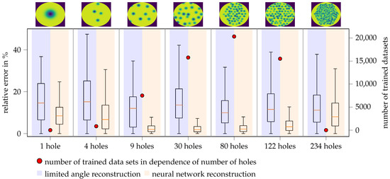
Figure 10.
Limited angle and neural network extrapolated error distribution of tomographic reconstruction in dependency of model complexity.
For a very simple model with only few resonators, the neural network reconstruction distribution error is a factor of 2 higher than reconstructions with higher complexity starting at nine holes. We assume that this effect is caused by a small number of trained data sets with a corresponding number of holes, because the focus of the training data is on a higher number of holes. At an average number of holes of 9 to 80 resonators, the neural network reconstruction distribution errors are very low and are below 4.5%. For 122 resonators and above, the neural network reconstruction distribution error increases again and is at a comparable level to that at low complexity. We assume that the resolution of the sinogram is to low in relation to its complexity. This results in averaging errors within a pixel and consequently in reconstruction errors compared to limited angle filtered back projection. The neural network always shows improvement over the limited angle reconstruction, even if only a limited number of training sets existed. However, the increasing uncertainty for lowly represented training sets indicates that network training always needs to be performed on structures similar to the specimen.
4.2. Measurement Data
For validation the neural network, trained on synthetic data, was employed on experimental data. The measurements, shown here, were performed at the resonance frequency of the Helmholtz resonators at Hz. Some resonators were deactivated by filling resonator volume with liquid, to avoid a hexagonal rotational symmetry.
The first row of Figure 11 shows the sinograms with the full scanning angle (a), limited scanning angle (b) and the neuronal network based extrapolation (c). To get the limited angle sinogram, the outer angles in the scan range [0, 40] as well as [140, 180] were removed. The second row shows corresponding filtered back projection of the sinograms (d–f). The bottom row describes the relative error referred to the full angle filtered back projection tomographic reconstruction. The local error for limited angle and neural network reconstruction are depicted in (h,i). Boxplots at (g), show the corresponding error distribution. In addition, the location of the active resonators were marked in each case in the reconstruction.
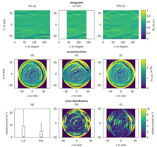
Figure 11.
Measured sound pressure field reconstruction: (a) full angle (FA) sinogram; (b) limited angle (LA) sinogram; (c) neural network (NN) extrapolated sinogram; (d) full angle filtered back projection tomographic reconstruction; (e) limited angle filtered back projection tomographic reconstruction; (f) neural network extrapolated filtered back projection tomographic reconstruction; (g) error distribution of local reconstructions compared to full angle reconstruction; (h) local error of limited angle reconstruction compared to full angle reconstruction; (i) local error of neural network reconstruction compared to full angle reconstruction.
In Figure 11, artifacts due to stitching the measurements can be seen. This results in horizontal lines in the sinograms (a–c) and circles in the reconstructions (d–f). Furthermore, strong distortions for radii above 45 mm due to the optical aberrations induced from the glass cylinder are apparent.
In the full angle reconstruction (d), a reduction of the sound pressure by 0.4 Pa can be seen above each active resonator. The resonators have a circular contour. The deactivated resonators can also be seen clearly. There is no characteristic minimum in the area above the resonator. That means this area has no local acoustic damping effect. The limited angle reconstruction (e) shows similar artifacts to the reconstruction of synthetic data, additionally to the measurement artifacts, mentioned in the full angle reconstruction. Line artifacts, as well as amplitude errors, are present. The contours of the resonators are elliptical. The amplitude over the resonators reconstructed with limited angle deviates by 0.23 Pa compared to the full angle reconstruction.
The sinogram of the neural network extrapolated data (c) shows a hard transition from the extrapolated angular scan range. There is a spatial low-pass effect in the extrapolation. However, this reconstruction (f) also shows a significant improvement compared to the limited angle reconstruction. The contour of the resonator is round and artifacts are strongly attenuated. The amplitude over the resonators reconstructed with neural network extrapolation deviates by 0.05 Pa compared to the full angle reconstruction.
The comparison of the limited angle and neural network with the full angle reconstruction shows that, overall, a significant reduction in relative error distribution can be achieved with the neural network extrapolated sinogram. Especially, in a close range around the Plexiglas wall an error reduction with neural network reconstruction is noticeable. Local errors surrounding the position of local resonators, are present in Figure 11h. This means every hole has a significant local sound pressure error compared to the full angle reconstruction. In neural network comparison (i), there is no error surrounding the position of local resonators. Thus, it can be assumed that the reconstruction of a single hole is almost similar compared to the full angle reconstruction.
The associated distribution error is presented in Figure 11g. The mean error can be reduced from 3.5% to 2.6% and maximum error can be reduced from 22.13% to 11.34%. The reconstruction improvement is lower than the synthetic model. We assume this is caused by measurement artifacts and deviation of the model used for physical boundary conditions.
5. Summary and Outlook
Limited angle tomography is important for many applications, especially at technical processes but suffers from artifacts and unknown measurement deviations. The hypothesis of the approach of extrapolation of non-scannable angular regions through an neural network with only synthetic data sets used for training can be confirmed. We show that we can reduce the MSE by a factor of 2.24 and the maximum error by a factor of 2.22 on synthetic data and reduce the MSE by a factor of 1.93 and the maximum error by 1.95 when evaluating measurement data. The dense Unet was applied to real measurement data acquired with a high-speed camera-based laser interferometric vibrometer on a bias flow liner model. The measurements validate the approach, demonstrating the big potential for this technology to generate a paradigm shift in limited angle tomography. Using the neural network for extrapolation only, is a simple extension and easier to implement compared to using neural networks for the complete tomographic reconstruction. Established signal processing only needs to be extended with this technique and has not to be changed completely.
Further investigation is required into the translation of this technique to other specimen and structures especially regarding their sparseness and complexity. In the next steps, the approach can be further improved. We want to use 3D data for extrapolation. By doing so, the measurement artifacts could be minimized, resulting in more appropriate information to feed in the neural network for extrapolation. In addition, more complex structures have to be trained. Finally the approach will be applied at real flow channel measurements.
Author Contributions
Conceptualization, O.R., J.G., R.K. and J.C.; methodology, O.R. and J.G.; software, O.R.; validation, O.R.; formal analysis, O.R.; investigation, O.R. and J.G.; data curation, O.R.; writing—original draft preparation, O.R.; writing—review and editing, J.G., J.C. and R.K.; visualization, O.R. and J.G.; supervision, J.C. and R.K.; project administration, O.R. and R.K.; funding acquisition, J.G., R.K. and J.C. All authors have read and agreed to the published version of the manuscript.
Funding
This research was funded by the Deutsche Forschungsgemeinschaft (DFG) grant number CZ55/41-1.
Institutional Review Board Statement
Not applicable.
Informed Consent Statement
Not applicable.
Data Availability Statement
The data presented in this study are available on request from the corresponding author. The data are not publicly available due to its large amount. It is stored locally and will be made accessible via cloud sharing after request.
Acknowledgments
The authors would like to thank our partners Lars Enghardt, Friedrich Bake and Larisa Grizewski from TU Berlin and the Deutsches Zentrum für Luft- und Raumfahrt (DLR), Berlin, Germany.
Conflicts of Interest
The authors declare no conflict of interest.
References
- Kiefhaber, S.; Rosenbaum, M.; Sauer-Greff, W.; Urbansky, R. A relation between algebraic and transform-based reconstruction technique in computed tomography. Adv. Radio Sci. 2013, 11, 95–100. [Google Scholar] [CrossRef]
- Kalke, M.; Siltanen, S. Sinogram Interpolation Method for Sparse-Angle Tomography. Appl. Math. 2014, 05, 423–441. [Google Scholar] [CrossRef]
- Wu, Z.; Zhu, Y.; Li, L.; Yang, T. Feature-based sparse angle tomography reconstruction for dynamic characterization of bio-cellular materials. In Computer Imaging III; SPIE: Orlando, FL, USA, 2018; p. 22. [Google Scholar] [CrossRef]
- Ayoub, A.B.; Pham, T.A.; Lim, J.; Unser, M.; Psaltis, D. A method for assessing the fidelity of optical diffraction tomography reconstruction methods using structured illumination. Opt. Commun. 2020, 454, 124486. [Google Scholar] [CrossRef]
- Yalavarthy, P.K.; Pogue, B.W.; Dehghani, H.; Carpenter, C.M.; Jiang, S.; Paulsen, K.D. Structural information within regularization matrices improves near infrared diffuse optical tomography. Opt. Express 2007, 15, 8043. [Google Scholar] [CrossRef]
- Zhang, X.; Curtis, A. Seismic Tomography Using Variational Inference Methods. J. Geophys. Res. Solid Earth 2020, 125. [Google Scholar] [CrossRef]
- Gürtler, J.; Greiffenhagen, F.; Woisetschläger, J.; Kuschmierz, R.; Czarske, J. Seedingless measurement of density fluctuations and flow velocity using high-speed holographic interferometry in a swirl-stabilized flame. Opt. Lasers Eng. 2020, 06481. [Google Scholar] [CrossRef]
- Kupsch, A.; Lange, A.; Hentschel, M.P.; Manke, I.; Kardjilov, N.; Arlt, T.; Grothausmann, R. Rekonstruktion limitierter CT-Messdatensätze von Brennstoffzellen mit Directt. Mater. Test. 2010, 52, 676–683. [Google Scholar] [CrossRef]
- Ramos Ruiz, A.E.; Gürtler, J.; Kuschmierz, R.; Czarske, J.W. Measurement of the Local Sound Pressure on a Bias-Flow Liner Using High-Speed Holography and Tomographic Reconstruction. IEEE Access 2019, 7, 153466–153474. [Google Scholar] [CrossRef]
- Torras-Rosell, A.; Barrera-Figueroa, S.; Jacobsen, F. Sound field reconstruction using acousto-optic tomography. J. Acoust. Soc. Am. 2012, 131, 3786–3793. [Google Scholar] [CrossRef] [PubMed]
- Haufe, D.; Gürtler, J.; Schulz, A.; Bake, F.; Enghardt, L.; Czarske, J. Aeroacoustic analysis using natural Helmholtz–Hodge decomposition. J. Sens. Sens. Syst. 2018, 7, 113–122. [Google Scholar] [CrossRef]
- Heuwinkel, C.; Piot, E.; Micheli, F.; Fischer, A.; Enghardt, L.; Bake, F.; Röhle, I. Characterization of a Perforated Liner by Acoustic and Optical Measurements. In Proceedings of the 16th AIAA/CEAS Aeroacoustics Conference, Stockholm, Sweden, 7–9 June 2010; pp. 1–15. [Google Scholar] [CrossRef]
- Abernathy, D.L.; Stone, M.B.; Loguillo, M.J.; Lucas, M.S.; Delaire, O.; Tang, X.; Lin, J.Y.Y.; Fultz, B. Design and operation of the wide angular-range chopper spectrometer ARCS at the Spallation Neutron Source. Rev. Sci. Instrum. 2012, 83, 015114. [Google Scholar] [CrossRef] [PubMed]
- Huang, Y.; Huang, X.; Taubmann, O.; Xia, Y.; Haase, V.; Hornegger, J.; Lauritsch, G.; Maier, A. Restoration of missing data in limited angle tomography based on Helgason—Ludwig consistency conditions. Biomed. Phys. Eng. Express 2017, 3, 035015. [Google Scholar] [CrossRef]
- Kadu, A.; Mansour, H.; Boufounos, P.T. High-Contrast Reflection Tomography With Total-Variation Constraints. IEEE Trans. Comput. Imaging 2020, 6, 1523–1536. [Google Scholar] [CrossRef]
- Zhang, H.; Li, L.; Qiao, K.; Wang, L.; Yan, B.; Li, L.; Hu, G. Image Prediction for Limited-angle Tomography via Deep Learning with Convolutional Neural Network. arXiv 2016, arXiv:1607.08707. [Google Scholar]
- Frikel, J.; Quinto, E.T. Characterization and reduction of artifacts in limited angle tomography. Inverse Probl. 2013, 29, 125007. [Google Scholar] [CrossRef]
- Assili, S. A Review of Tomographic Reconstruction Techniques for Computed Tomography. arXiv 2018, arXiv:1808.09172. [Google Scholar]
- Zhang, Z.; Liang, X.; Dong, X.; Xie, Y.; Cao, G. A Sparse-View CT Reconstruction Method Based on Combination of DenseNet and Deconvolution. IEEE Trans. Med. Imaging 2018, 37, 1407–1417. [Google Scholar] [CrossRef]
- Dong, J.; Fu, J.; He, Z. A deep learning reconstruction framework for X-ray computed tomography with incomplete data. PLoS ONE 2019, 14, e0224426. [Google Scholar] [CrossRef]
- McCann, M.T.; Jin, K.H.; Unser, M. Convolutional Neural Networks for Inverse Problems in Imaging: A Review. IEEE Signal Process. Mag. 2017, 34, 85–95. [Google Scholar] [CrossRef]
- Pham, T.A.; Soubies, E.; Ayoub, A.; Psaltis, D.; Unser, M. Adaptive Regularization for Three-Dimensional Optical Diffraction Tomography. In Proceedings of the 2020 IEEE 17th International Symposium on Biomedical Imaging, Iowa City, IA, USA, 3–7 April 2020; pp. 182–186. [Google Scholar] [CrossRef]
- Zhou, K.C.; Horstmeyer, R. Diffraction tomography with a deep image prior. Opt. Express 2020, 28, 12872. [Google Scholar] [CrossRef]
- Allen, C.S.; Blake, W.K.; Dougherty, R.P.; Lynch, D.; Soderman, P.T.; Underbrink, J.R. Aeroacoustic Measurements; Springer: Berlin/Heidelberg, Germany, 2002. [Google Scholar] [CrossRef]
- Rafaely, B. Analysis and design of spherical microphone arrays. IEEE Trans. Speech Audio Process. 2005, 13, 135–143. [Google Scholar] [CrossRef]
- Hoffmann, M.; Unger, A.; Jager, A.; Kupnik, M. Effect of transducer port cavities in invasive ultrasonic transit-time gas flowmeters. In Proceedings of the 2015 IEEE International Ultrasonics Symposium, Taipei, Taiwan, 21–24 October 2015; pp. 1–4. [Google Scholar] [CrossRef]
- Choi, H.; Park, J.; Lim, W.; Yang, Y.M. Active-beacon-based driver sound separation system for autonomous vehicle applications. Appl. Acoust. 2021, 171, 107549. [Google Scholar] [CrossRef]
- Meyer, J.; Elko, G. A highly scalable spherical microphone array based on an orthonormal decomposition of the soundfield. In Proceedings of the IEEE International Conference on Acoustics, Speech, and Signal Processing, Orlando, FL, USA, 13–17 May 2002; pp. II-1781–II-1784. [Google Scholar] [CrossRef]
- Greiffenhagen, F.; Woisetschläger, J.; Gürtler, J.; Czarske, J. Quantitative measurement of density fluctuations with a full-field laser interferometric vibrometer. Exp. Fluids 2020, 61, 9. [Google Scholar] [CrossRef]
- Greiffenhagen, F.; Peterleithner, J.; Woisetschläger, J.; Fischer, A.; Gürtler, J.; Czarske, J. Discussion of laser interferometric vibrometry for the determination of heat release fluctuations in an unconfined swirl-stabilized flame. Combust. Flame 2019, 201, 315–327. [Google Scholar] [CrossRef]
- Prabhat, P.; Arumugam, S.; Madan, V. FilteringinFiltered Backprojection Computerized Tomography. In Proceedings of the National Conference “NCNTE-2012” at Fr. CRIT, Vashi, Navi Mumbai, India, 24–25 February 2012. [Google Scholar] [CrossRef]
- Lim, J.; Lee, K.; Jin, K.H.; Shin, S.; Lee, S.; Park, Y.; Ye, J.C. Comparative study of iterative reconstruction algorithms for missing cone problems in optical diffraction tomography. Opt. Express 2015, 23, 16933. [Google Scholar] [CrossRef] [PubMed]
- Khan, A.; Sohail, A.; Zahoora, U.; Qureshi, A.S. A survey of the recent architectures of deep convolutional neural networks. Artif. Intell. Rev. 2020, 53, 5455–5516. [Google Scholar] [CrossRef]
- Ronneberger, O.; Fischer, P.; Brox, T. U-Net: Convolutional Networks for Biomedical Image Segmentation. In Proceedings of the Medical Image Computing and Computer-Assisted Intervention—MICCAI 2015, Munich, Germany, 5–9 October 2015; pp. 34–241. [Google Scholar] [CrossRef]
- Rothe, S.; Zhang, Q.; Koukourakis, N.; Czarske, J. Intensity-Only Mode Decomposition on Multimode Fibers Using a Densely Connected Convolutional Network. J. Light. Technol. 2021, 39, 1672–1679. [Google Scholar] [CrossRef]
- Srivastava, N.; Hinton, G.; Krizhevsky, A.; Sutskever, I.; Salakhutdinov, R. Dropout: A simple way to prevent neural networks from overfitting. J. Mach. Learn. Res. 2014, 15, 1929–1958. [Google Scholar]
- Wang, Z.; Bovik, A.; Sheikh, H.; Simoncelli, E. Image Quality Assessment: From Error Visibility to Structural Similarity. IEEE Trans. Image Process. 2004, 13, 600–612. [Google Scholar] [CrossRef] [PubMed]
- Wang, J.; Zhang, Z.; Huang, Y.; Li, Z.; Huang, Q. A 3D convolutional neural network based near-field acoustical holography method with sparse sampling rate on measuring surface. Measurement 2021, 177, 109297. [Google Scholar] [CrossRef]
Publisher’s Note: MDPI stays neutral with regard to jurisdictional claims in published maps and institutional affiliations. |
© 2021 by the authors. Licensee MDPI, Basel, Switzerland. This article is an open access article distributed under the terms and conditions of the Creative Commons Attribution (CC BY) license (https://creativecommons.org/licenses/by/4.0/).