
Study of Image Classification Accuracy with Fourier Ptychography


 ,
, 
Abstract
1. Introduction
2. Methodology
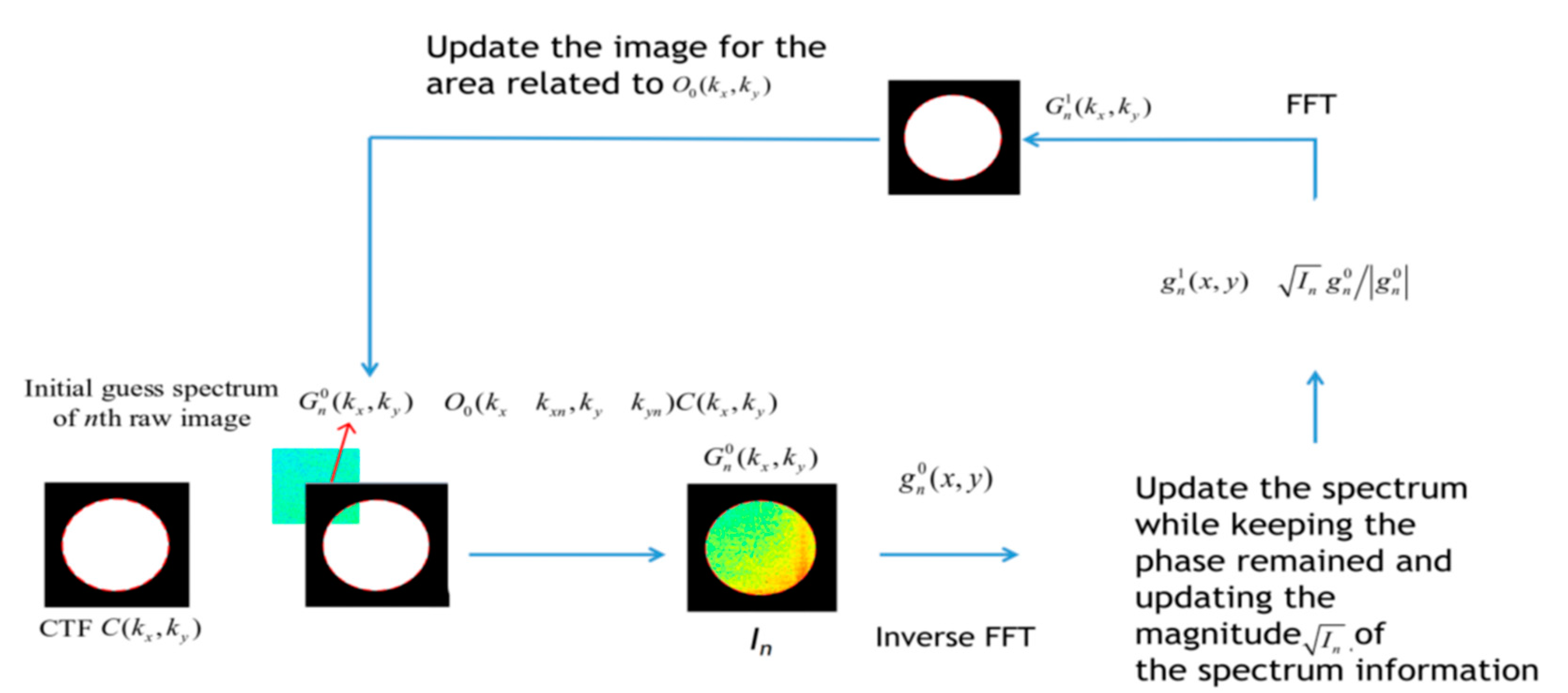
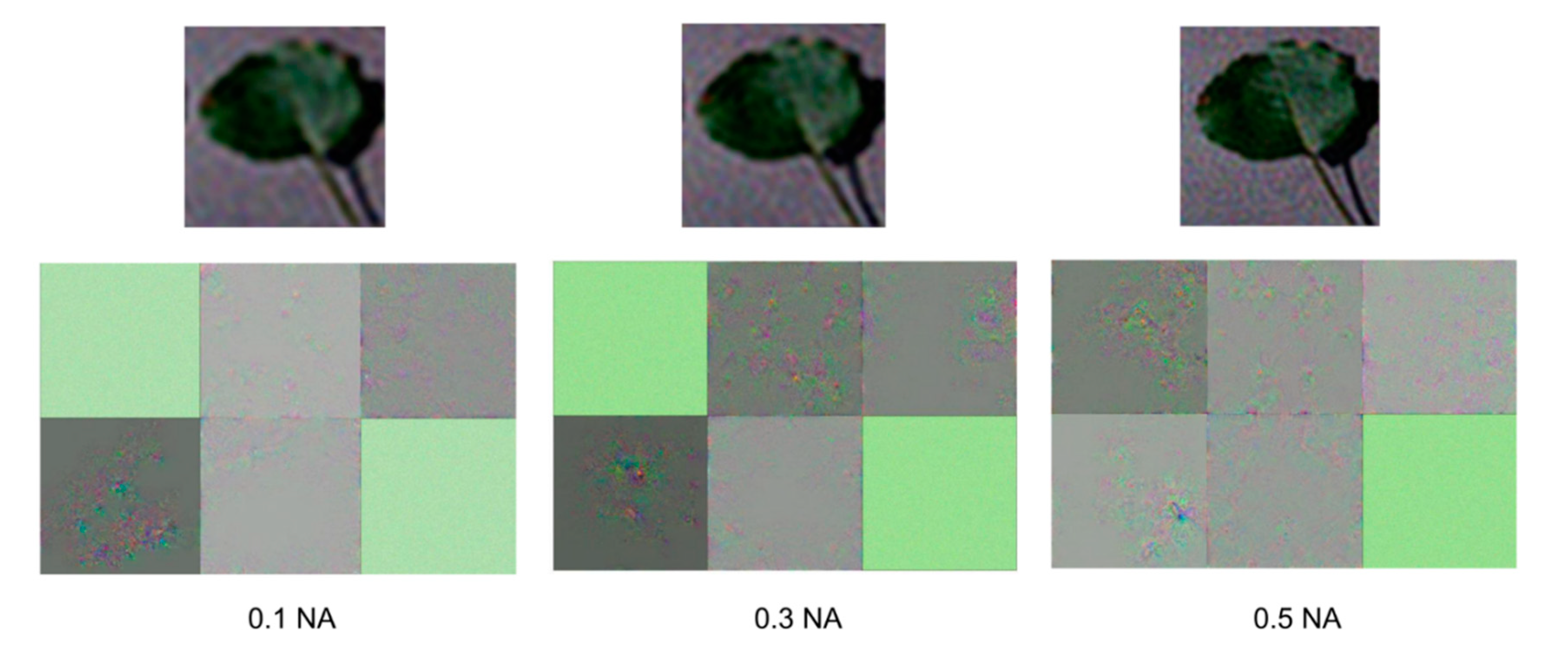
2.1. Fourier Ptychography
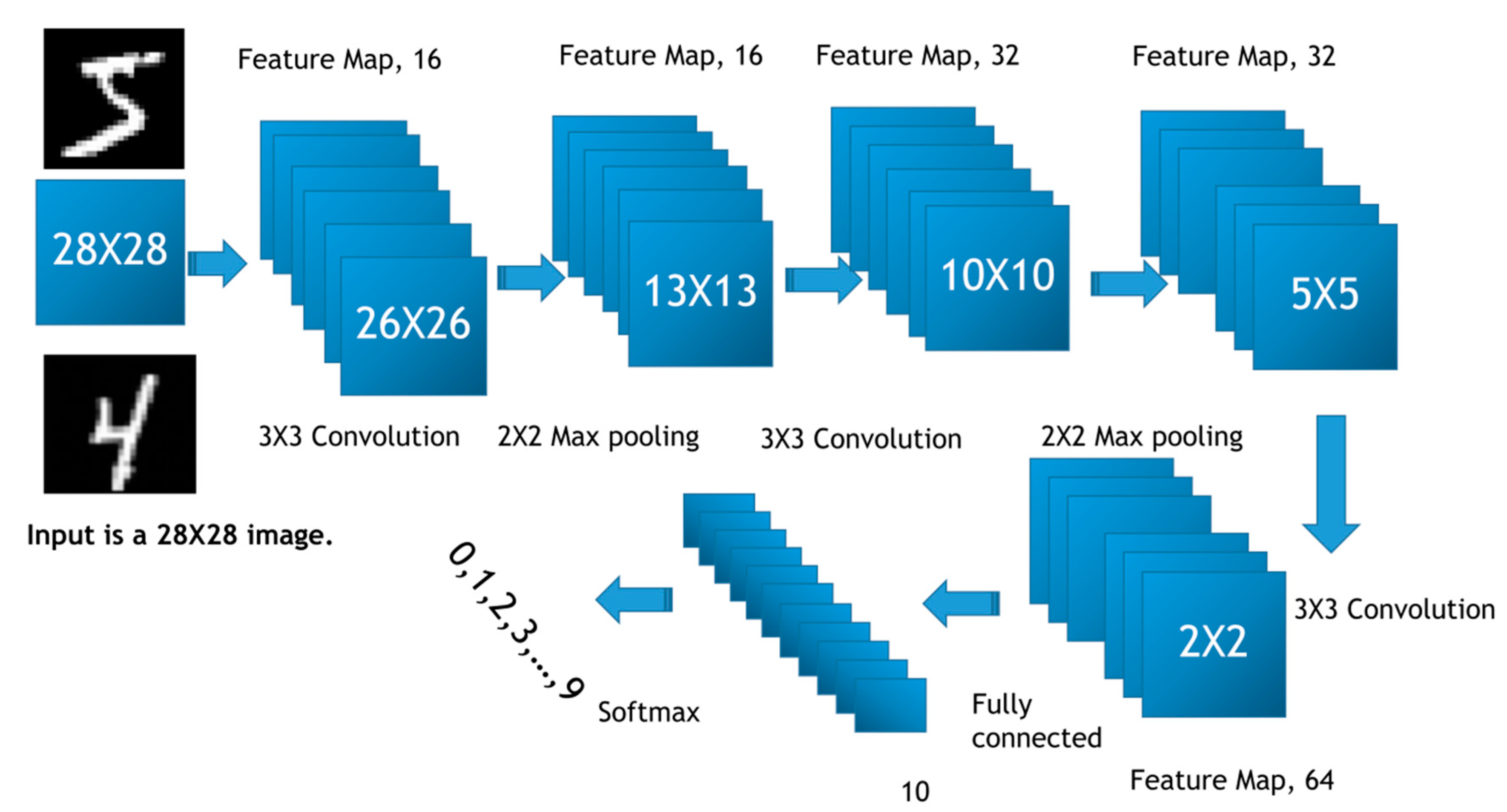
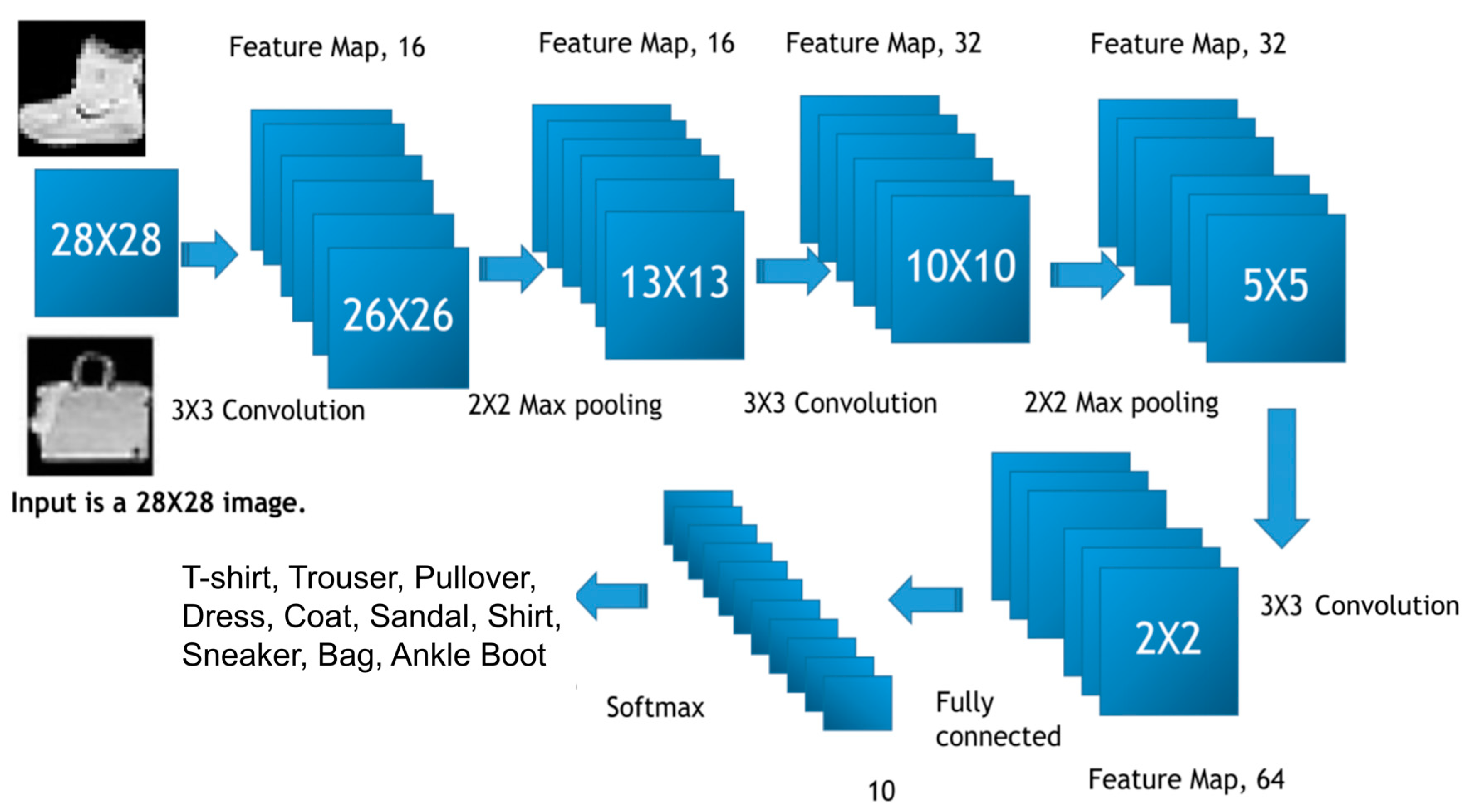
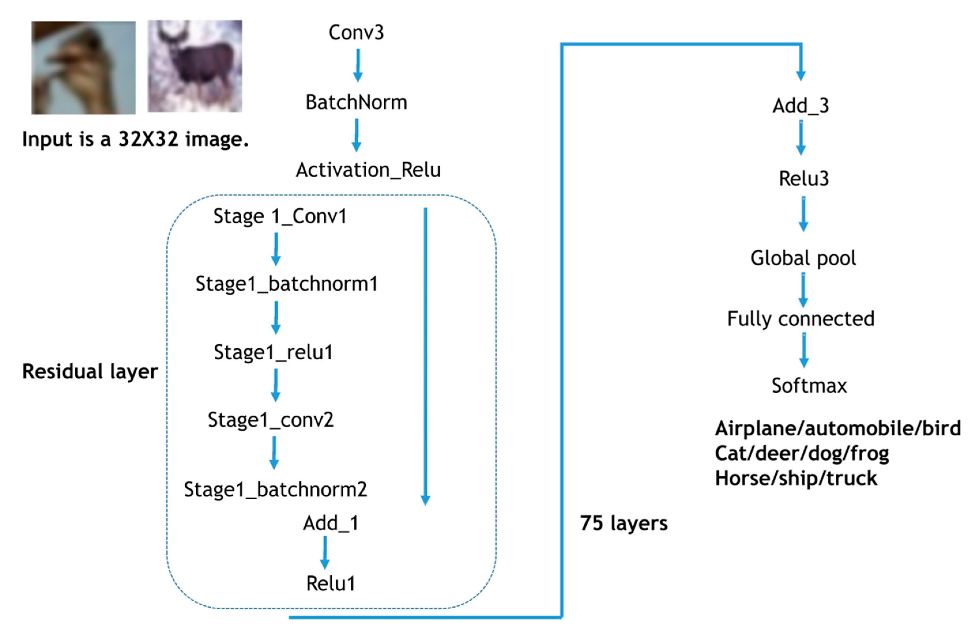
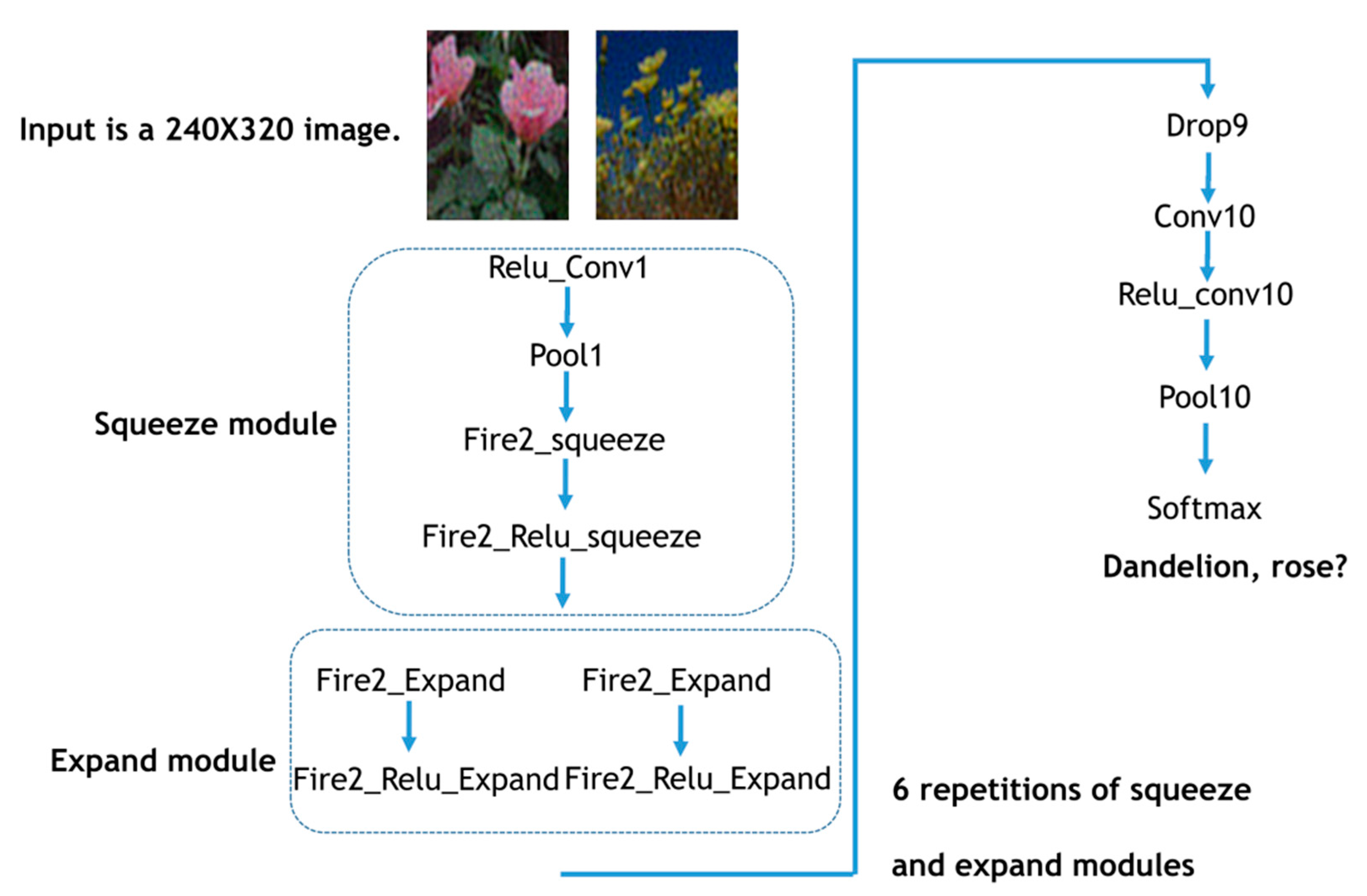
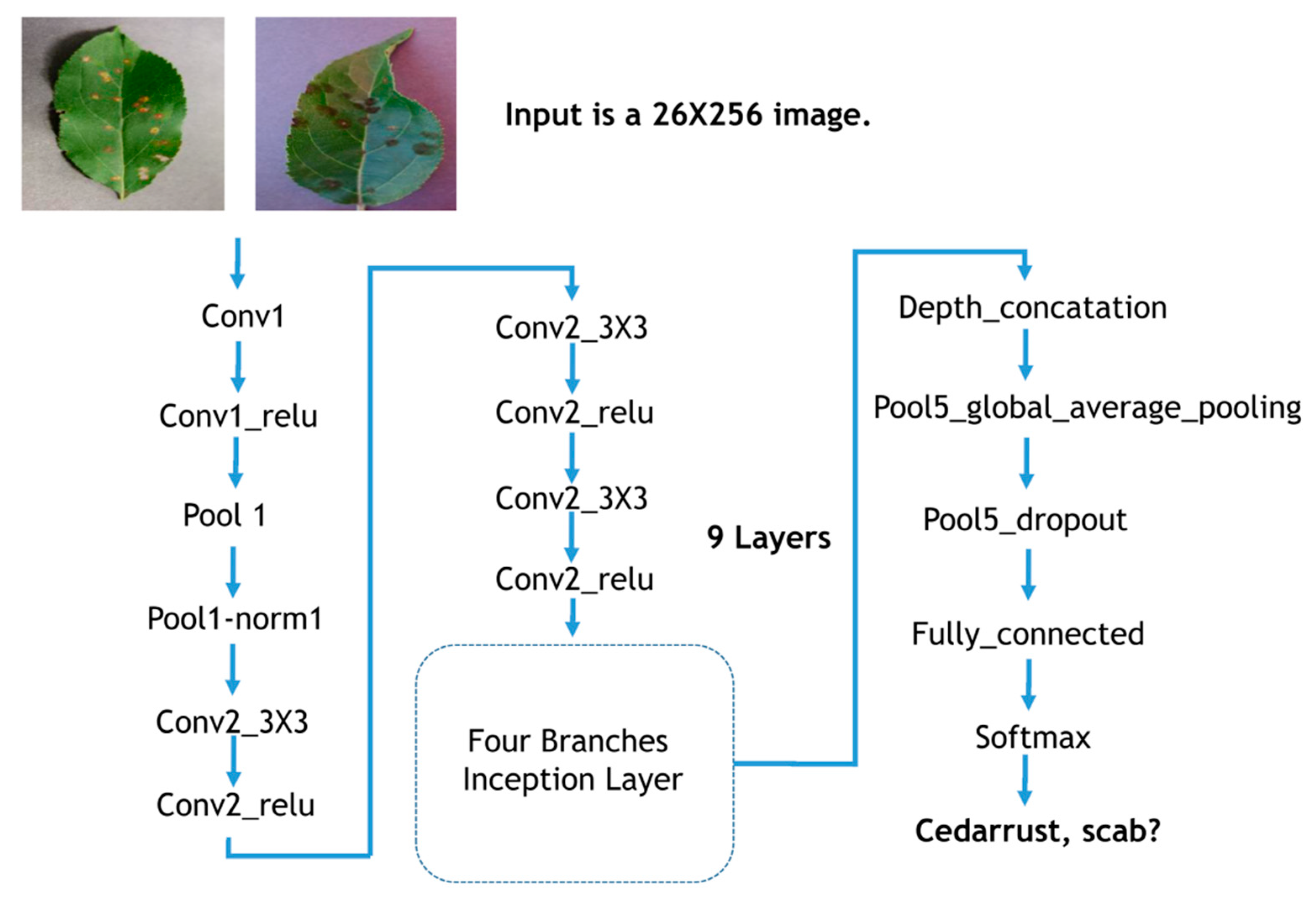
2.2. Image Classification
3. Results
4. Conclusions
Author Contributions
Funding
Institutional Review Board Statement
Informed Consent Statement
Data Availability Statement
Conflicts of Interest
References
- Zheng, G.; Horstmeyer, R.; Yang, C. Wide-field, high-resolution Fourier ptychographic microscopy. Nat. Photonic 2013, 7, 739–745. [Google Scholar] [CrossRef] [PubMed]
- Zheng, G.; Shen, C.; Jiang, S.; Song, P.; Yang, C. Concept, implementations and applications of Fourier ptychography. Nat. Rev. Phys. 2021, 3, 207–223. [Google Scholar] [CrossRef]
- Tian, L.; Li, X.; Ramchandran, K.; Waller, L. Multiplexed coded illumination for Fourier ptychography with an LED array microscope. Biomed. Opt. Express 2014, 5, 2376–2389. [Google Scholar] [CrossRef] [PubMed]
- Sun, J.; Chen, Q.; Zhang, J.; Fan, Y.; Zuo, C. Single-shot quantitative phase microscopy based on color-multiplexed Fourier ptychography. Opt. Lett. 2018, 43, 3365–3368. [Google Scholar] [CrossRef] [PubMed]
- Sun, J.; Zuo, C.; Zhang, J.; Fan, Y.; Chen, Q. High-speed Fourier ptychographic microscopy based on programmable annular illuminations. Sci. Rep. 2018, 8, 7669. [Google Scholar] [CrossRef] [PubMed]
- Jiang, S.; Guo, K.; Liao, J.; Zheng, G. Solving Fourier ptychographic imaging problems via neural network modeling and TensorFlow. Biomed. Opt. Express 2018, 9, 3306–3319. [Google Scholar] [CrossRef] [PubMed]
- Nguyen, T.; Xue, Y.; Li, Y.; Tian, L.; Nehmetallah, G. Deep learning approach for Fourier ptychography microscopy. Opt. Express 2018, 26, 26470–26484. [Google Scholar] [CrossRef] [PubMed]
- Chen, L.; Wu, Y.; Souza, A.M.D.; Abidin, A.Z.; Wismüller, A.; Xu, C. MRI tumor segmentation with densely connected 3D CNN. In Proceedings of the Medical Imaging 2018: Image Processing, (International Society for Optics and Photonics), Houston, TX, USA, 11–13 February 2018; Volume 105741F. [Google Scholar]
- Zhu, P.; Wen, L.; Bian, X.; Ling, H.; Hu, Q. Vision meets drones: A challenge. arXiv 2018, arXiv:1804.07437. [Google Scholar]
- Goyal, P.; Dollár, P.; Girshick, R.; Noordhuis, P.; Wesolowski, L.; Kyrola, A.; Tulloch, A.; Jia, Y.; He, K. Accurate, Large Minibatch SGD: Training ImageNet in 1 Hour. arXiv 2017, arXiv:1706.02677. [Google Scholar]
- Zhang, H.; Zhou, W.-J.; Liu, Y.; Leber, D.; Banerjee, P.; Basunia, M.; Poon, T.-C. Evaluation of finite difference and FFT-based solutions of the transport of intensity equation. Appl. Opt. 2017, 57, A222–A228. [Google Scholar] [CrossRef] [PubMed]
- Zhou, W.-J.; Guan, X.; Liu, F.; Yu, Y.; Zhang, H.; Poon, T.-C.; Banerjee, P.P. Phase retrieval based on transport of intensity and digital holography. Appl. Opt. 2018, 57, A229–A234. [Google Scholar] [CrossRef] [PubMed]
- Zhang, H.; Zhou, W.; Leber, D.; Hu, Z.; Yang, X.; Tsang, P.W.M.; Poon, T.-C. Development of lossy and near-lossless compression methods for wafer surface structure digital holograms. J. Micro/Nanolithogr. MEMS MOEMS 2015, 14, 41304. [Google Scholar] [CrossRef]
- Xiao, H.; Rasul, K.; Vollgraf, R. Fashion-MNIST: A novel image dataset for benchmarking machine learning algorithms. arXiv 2017, arXiv:1708.07747. [Google Scholar]
- Zhong, Z.; Zheng, L.; Kang, G.; Li, S.; Yang, Y. Random erasing data augmentation. arXiv 2017, arXiv:1708.04896. [Google Scholar] [CrossRef]
- He, K.; Zhang, X.; Ren, S.; Sun, J. Deep residual learning for image recognition. In Proceedings of the IEEE Conference on Computer Vision and Pattern Recognition, Las Vegas, NV, USA, 27–30 June 2016; pp. 770–778. [Google Scholar]
- Perez, L.; Wang, J. The effectiveness of data augmentation in image classification using deep learning. arXiv 2017, arXiv:1712.04621. [Google Scholar]
- Zhong, Z.; Zheng, L.; Zheng, Z.; Li, S.; Yang, Y. Camera Style Adaptation for Person Re-identification. In Proceedings of the 2018 IEEE/CVF Conference on Computer Vision and Pattern Recognition, Salt Lake City, UT, USA, 18–22 June 2018; pp. 5157–5166. [Google Scholar]
- Wang, R.; Song, P.; Jiang, S.; Yan, C.; Zhu, J.; Guo, C.; Bian, Z.; Wang, T.; Zheng, G. Virtual brightfield and fluorescence staining for Fourier ptychography via unsupervised deep learning. Opt. Lett. 2020, 45, 5405–5408. [Google Scholar] [CrossRef] [PubMed]
- Li, Y.; Cheng, S.; Xue, Y.; Tian, L. Displacement-agnostic coherent imaging through scatter with an interpretable deep neural network. Opt. Express 2021, 29, 2244–2257. [Google Scholar] [CrossRef] [PubMed]
- Zhang, H.; Wang, L.; Zhou, W.; Hu, Z.; Tsang, P.; Poon, T.-C. Fourier Ptychography: Effectiveness of image classification. In Proceedings of the SPIE, Melbourne, Australia, 14–17 October 2019; Volume 11205, pp. 112050G-1–112050G-8. [Google Scholar]
- Wang, L.; Song, Q.; Zhang, H.; Yuan, C.; Poon, T.-C. Optical scanning Fourier ptychographic microscopy. Appl. Opt. 2021, 60, A243–A249. [Google Scholar] [CrossRef] [PubMed]
- Gowdra, N.; Sinha, R.; MacDonell, S. Examining convolutional feature extraction using Maximum Entropy (ME) and Signal-to-Noise Ratio (SNR) for image classification. In Proceedings of the IECON 2020 the 46th Annual Conference of the IEEE Industrial Electronics Society, Singapore, 18–22 October 2020; pp. 471–476. [Google Scholar]
- Li, Q.; Shen, L.; Guo, S.; Lai, Z. Wavelet Integrated CNNs for Noise-Robust Image Classification. In Proceedings of the IEEE/CVF Conference on Computer Vision and Pattern Recognition (CVPR), Seattle, WA, USA, 14–19 June 2020; pp. 7245–7254. [Google Scholar]


| Dataset | Numerical Aperture | Reconstruction Method | PSNR | SSIM | Classification Accuracy |
|---|---|---|---|---|---|
| CIFAR | Ground Truth | Inf | 1 | 76.61% | |
| 0.5 | FPM | 14.64 | 0.79 | 61.72% | |
| Lower Resolution | 14.39 | 0.76 | 58.79% | ||
| 0.2 | FPM | 14.46 | 0.78 | 59.38% | |
| Lower Resolution | 13.81 | 0.61 | 52.74% | ||
| 0.05 | FPM | 12.48 | 0.33 | 42.39% | |
| Lower Resolution | 12.06 | 0.31 | 35.16% | ||
| CalTech 101 | Ground Truth | Inf | 1 | 91.75% | |
| 0.5 | FPM | 13.37 | 0.52 | 73.75% | |
| Lower Resolution | 12.82 | 0.50 | 61.50% | ||
| 0.2 | FPM | 13.11 | 0.53 | 65.50% | |
| Lower Resolution | 12.44 | 0.49 | 36.25% | ||
| 0.05 | FPM | 11.09 | 0.31 | 20.00% | |
| Lower Resolution | 10.69 | 0.38 | 4.75% | ||
| Dataset | Numerical Aperture | Reconstruction Method | PSNR | SSIM | Classification Accuracy |
|---|---|---|---|---|---|
| MNIST | Ground Truth | Inf | 1 | 96.87% | |
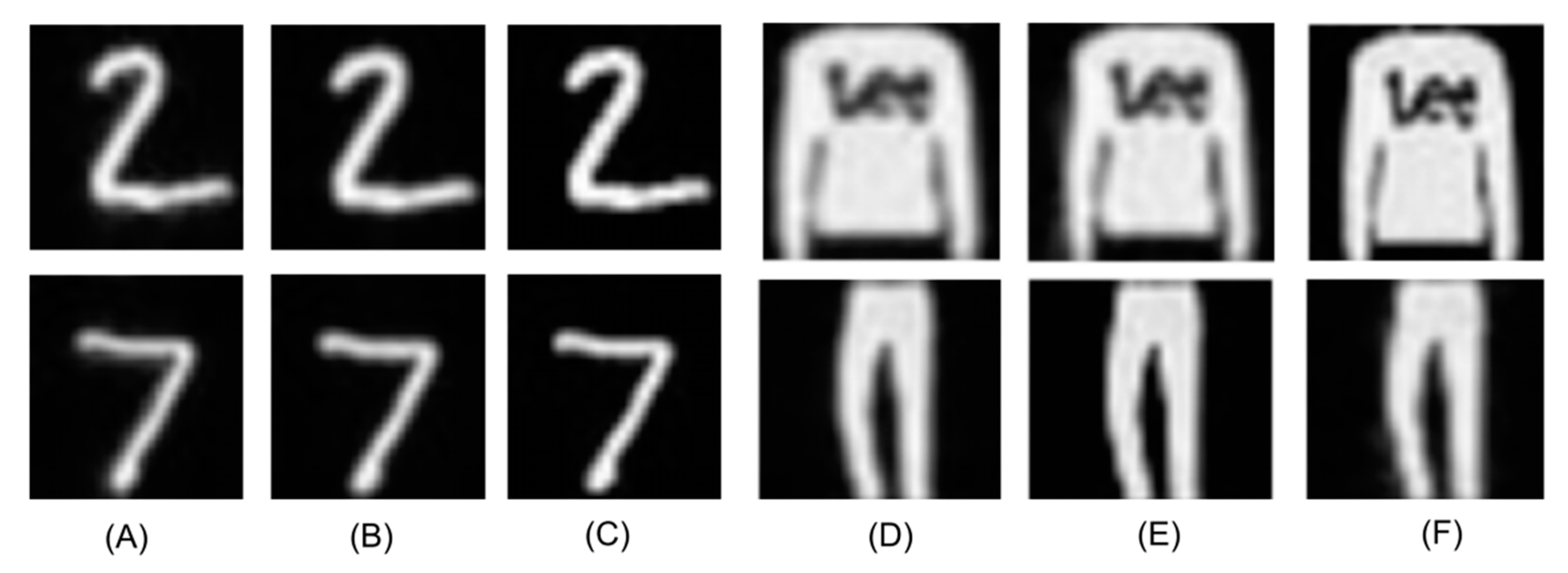
| 0.5 | FPM | 27.82 | 0.84 | 96.29% | |
| Lower Resolution | 22.11 | 0.53 | 95.89% | ||
| 0.2 | FPM | 23.99 | 0.63 | 97.66% | |
| Lower Resolution | 16.81 | 0.33 | 94.73% | ||
| 0.05 | FPM | 12.12 | 0.13 | 89.06% | |
| Lower Resolution | 11.58 | 0.05 | 62.50% | ||
| Fashion MNIST | Ground Truth | Inf | 1 | 85.35% | |
| 0.5 | FPM | 26.88 | 0.88 | 84.57% | |
| Lower Resolution | 22.69 | 0.72 | 83.59% | ||
| 0.2 | FPM | 23.88 | 0.76 | 83.20% | |
| Lower Resolution | 17.50 | 0.47 | 83.01% | ||
| 0.05 | FPM | 11.96 | 0.19 | 78.23% | |
| Lower Resolution | 11.94 | 0.11 | 67.58% | ||
| Dataset | Numerical Aperture | Reconstruction Method | PSNR | SSIM | Classification Accuracy |
|---|---|---|---|---|---|
| Flowers | Ground Truth | Inf | 1 | 83.15% | |
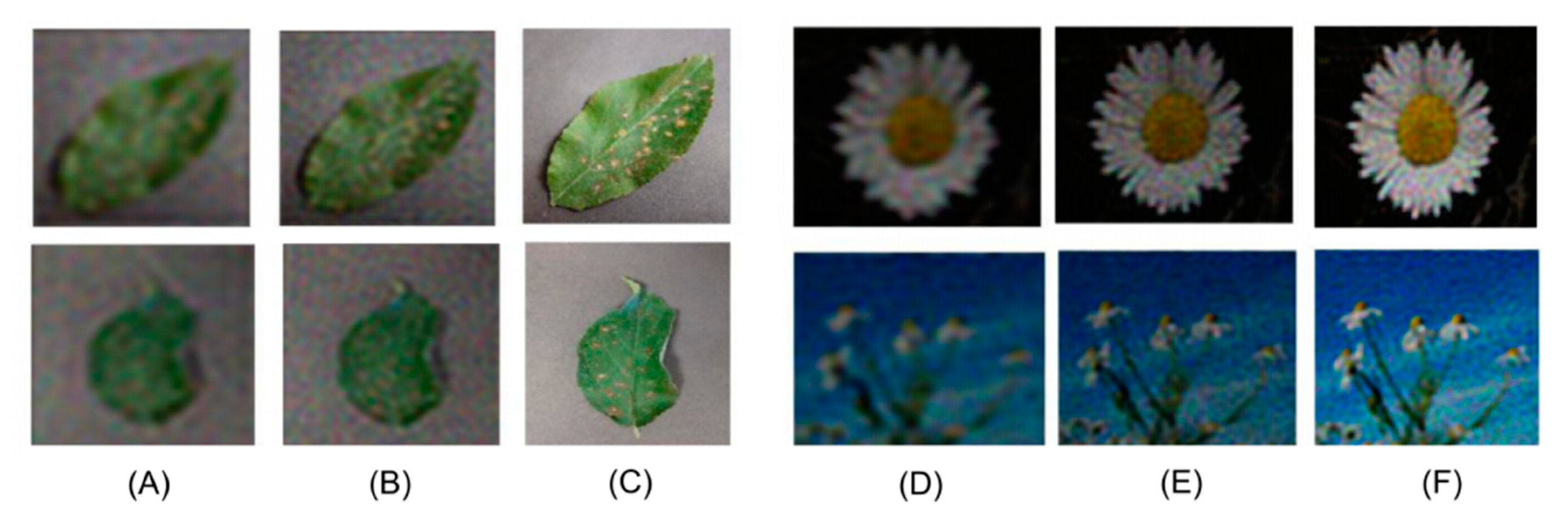
| 0.5 | FPM | 19.26 | 0.80 | 81.25% | |
| Lower Resolution | 18.42 | 0.68 | 74.19% | ||
| 0.2 | FPM | 18.66 | 0.70 | 76.30% | |
| Lower Resolution | 17.35 | 0.59 | 72.14% | ||
| 0.05 | FPM | 16.02 | 0.41 | 70.28% | |
| Lower Resolution | 15.33 | 0.47 | 49.18% | ||
| Apple Pathology | Ground Truth | Inf | 1 | 99.56% | |
| 0.5 | FPM | 15.44 | 0.62 | 98.12% | |
| Lower Resolution | 15.32 | 0.66 | 97.32% | ||
| 0.2 | FPM | 15.28 | 0.66 | 91.23% | |
| Lower Resolution | 14.98 | 0.67 | 89.19% | ||
| 0.05 | FPM | 6.71 | 0.0082 | 90.12% | |
| Lower Resolution | 6.64 | 0.0003 | 82.35% | ||
| Multiple Linear Regression p-Value | p-Value | Statistical Significance (p < 0.05) |
|---|---|---|
| MNIST | 0.0046 | Yes |
| Fashion-MNIST | 3.02 × 10⁻⁵ | Yes |
| CIFAR | 0.02 | Yes |
| CalTech101 | 1.87 × 10⁻⁶ | Yes |
| Flowers | 0.0032 | Yes |
| Apple Pathology | 0.04 | Yes |
Publisher’s Note: MDPI stays neutral with regard to jurisdictional claims in published maps and institutional affiliations. |
© 2021 by the authors. Licensee MDPI, Basel, Switzerland. This article is an open access article distributed under the terms and conditions of the Creative Commons Attribution (CC BY) license (https://creativecommons.org/licenses/by/4.0/).
Share and Cite
Zhang, H.; Zhang, Y.; Wang, L.; Hu, Z.; Zhou, W.; Tsang, P.W.M.; Cao, D.; Poon, T.-C. Study of Image Classification Accuracy with Fourier Ptychography. Appl. Sci. 2021, 11, 4500. https://doi.org/10.3390/app11104500
Zhang H, Zhang Y, Wang L, Hu Z, Zhou W, Tsang PWM, Cao D, Poon T-C. Study of Image Classification Accuracy with Fourier Ptychography. Applied Sciences. 2021; 11(10):4500. https://doi.org/10.3390/app11104500
Chicago/Turabian StyleZhang, Hongbo, Yaping Zhang, Lin Wang, Zhijuan Hu, Wenjing Zhou, Peter W. M. Tsang, Deng Cao, and Ting-Chung Poon. 2021. "Study of Image Classification Accuracy with Fourier Ptychography" Applied Sciences 11, no. 10: 4500. https://doi.org/10.3390/app11104500
APA StyleZhang, H., Zhang, Y., Wang, L., Hu, Z., Zhou, W., Tsang, P. W. M., Cao, D., & Poon, T.-C. (2021). Study of Image Classification Accuracy with Fourier Ptychography. Applied Sciences, 11(10), 4500. https://doi.org/10.3390/app11104500