Dynamic Plan Control: An Effective Tool to Manage Demand Considering Mobile Internet Network Congestion

Abstract

Rapidly increasing mobile data traffic have placed a significant burden on mobile Internet networks. Due to limited network capacity, a mobile network is congested when it handles too much data traffic simultaneously. In turn, some customers leave the network, which induces a revenue loss for the mobile service provider. To manage demand and maximize revenue, we propose a dynamic plan control method for the mobile service providers under connection-speed-restriction pricing. This method allows the mobile service provider to dynamically set the data plans’ availability for potential customers’ new subscriptions. With dynamic plan control, the service provider can adjust data network utilization and achieve high customer satisfaction and a low churn rate, which reflect high service supply chain performance. To find the optimal control policy, we transform the high-dimensional dynamic programming problem into an equivalent mixed integer linear programming problem. We find that dynamic plan control is an effective tool for managing demand and increasing revenue in the long term. Numerical evaluation with a large European mobile service provider further supports our conclusion. Furthermore, when network capacity or potential customers’ willingness to join the network changes, the dynamic plan control method generates robust revenue for the service provider.

1. Introduction

Mobile data traffic have exploded with the wide popularity of mobile Internet service and the exponential growth of mobile applications. According to the Cisco Visual Networking Index released in February 2019 [1], global mobile data traffic have grown 17-fold from 2012 to 2017 and will continue growing at a compound annual growth rate (CAGR) of 46% from 2017 to 2022, reaching 77.5 exabytes per month by 2022. To handle rapidly increasing data traffic, new technology for wireless communications is needed. However, it takes a long time to promote technology. For example, the second-generation of wireless telecommunications technology (2G) appeared ten years before the third-generation (3G), followed by the fourth-generation (4G) eight years later. The fifth-generation of wireless telecommunications was developed fast, but it still took six years to finally launch 5G [2]. According to the technology characteristics, the capacity of the mobile network is fixed during the same generation of wireless telecommunications.

Customers use ever-increasing mobile Internet data while the mobile network capacity is fixed during several years of the same generation. As a consequence, limited mobile network capacity is threatened by immense data traffic. Specifically, when a mobile network handles too much data traffic simultaneously, network congestion occurs [3,4]. Network congestion leads to customer dissatisfaction in this wireless service supply chain. For example, Internet web pages cannot be displayed quickly, and videos cannot be played smoothly. In turn, customer dissatisfaction drives a number of customers to leave the wireless network and then influences the service provider’s revenue and the wireless service supply chain’s performance. Therefore, mobile service providers should take the potential network congestion into consideration while maximizing revenue [5]. To this end, several demand management methods considering congestion have been proposed and studied, such as time-of-day pricing [6] and Wi-Fi offloading [7]. A detailed discussion of these demand management methods is included in the literature review.

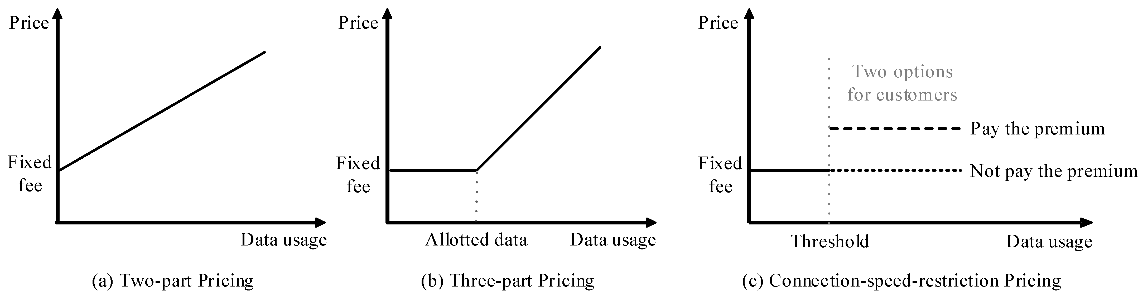
It is worth noting that the pricing scheme, where demand management methods apply, has evolved with the progression of wireless telecommunications technology. In the 1980s, the first-generation of wireless telecommunications technology (1G) was launched. Its connection speed was only $2.4$ Kb/s (1 Gb = 1024 Mb; 1 Mb = 1024 Kb), and users could only make voice calls. At this time, flat-rate pricing dominated, which charges each user a fixed fee per session independently of the user’s data usage. As wireless telecommunications technology upgraded to the second-generation (2G) and third-generation (3G), the connection speed could reach up to 10 Mb/s. Multimedia services emerged, such as the global positioning system (GPS) and video conferencing [8]. In the era of 2G and 3G, people used mobile Internet for different purposes, which made data usage vary greatly from one user to another. In 2011, the top 1% of mobile Internet users generated approximately 35% of the traffic over the world [9]. To better match a customer’s cost with her/his data usage, many service providers moved away from the simple flat-rate pricing to metered pricing, which charges a user in proportion to her/his data usage. In contrast to flat-rate pricing, metered pricing is concerned about not only whether a customer uses the data service, but also how much data she/he consumes.

Since the fourth-generation of wireless telecommunications technology (4G) was launched around 2009, connection speed has been greatly improved to 100 Mb/s. Mobile Internet service is fast becoming an integral part of people’s daily life and is used through various kinds of applications, including mobile videos, file transferring, social network services, etc. Most people already consider mobile Internet service as a necessity. In contrast to spending too much for mere access to mobile networks, people are more willing to pay for a high connection speed. This is where connection-speed-restriction pricing comes into play. Under connection-speed-restriction pricing, data usage is unlimited for users. However, when a user’s data usage exceeds a threshold in a billing period, her/his connection speed will be decreased. Throughout the rest of the current billing period, she/he can continue using mobile Internet, but at the restricted speed. To re-obtain full-speed mobile Internet service, the user needs to buy the supplementary data package or wait until the beginning of the next billing period. In contrast to flat-rate pricing and metered pricing, connection-speed-restriction pricing considers the connection speed, which is the focus for customer experience.

In practice, connection-speed-restriction pricing plays an increasingly important role in mobile Internet pricing. A study conducted on North American mobile service providers showed that the percentage of data plans offered under connection-speed-restriction pricing had grown from 39% in September 2016 to 66% in August 2018 [1]. In the arriving era of 5G, connection speed can reach up to 1 Gb/s, which is much faster than the speed of the 4G network. Hence, mobile service providers will have a strong motivation to employ connection-speed-restriction pricing in the 5G era.

Technically, the restriction of a user’s connection speed is achieved by shifting her/his data connection from a high-generation network to a low-generation network. For example, if a service provider uses a 5G network to provide full-speed data service, the restriction of a user’s connection speed can be achieved by shifting his/her data connection from a 5G network to a 3G network or even a 2G network. Most importantly, a 5G connection provides much higher connection speed than a 3G connection. According to Qualcomm’s experiment, a 5G connection provides over 100 times faster speed on average than a 3G connection. This fact provides valuable insight into demand management while considering network congestion. On the one hand, if too many customers buy the supplementary data package to use full-speed data service in the high-generation network, then the mobile network is highly prone to congestion. On the other hand, if too many customers do not buy the supplementary data package, then the service provider wastes the network capacity and loses potential revenue. Therefore, how can a wireless service provider manage demand and maximize revenue under connection-speed-restriction pricing? We explore this issue in our paper.

Based on connection-speed-restriction pricing, we propose a dynamic plan control method. With this method, a wireless service provider can dynamically control which data plans are open and which data plans are closed for new customers at the beginning of each period. Here, each period refers to one month, one quarter, or another time dimension according to the service provider’s state of operation. In each period, new customers can only subscribe to one of the open data plans. The close of a plan only prevents new customers from subscribing to it during a certain period, while old customers of this plan can still use and pay for it during this period. Therefore, the service provider can take the limited network capacity into consideration and maximize revenue in the long term by this dynamic plan control method. At the same time, customer experience is ensured, and supply chain performance is enhanced.

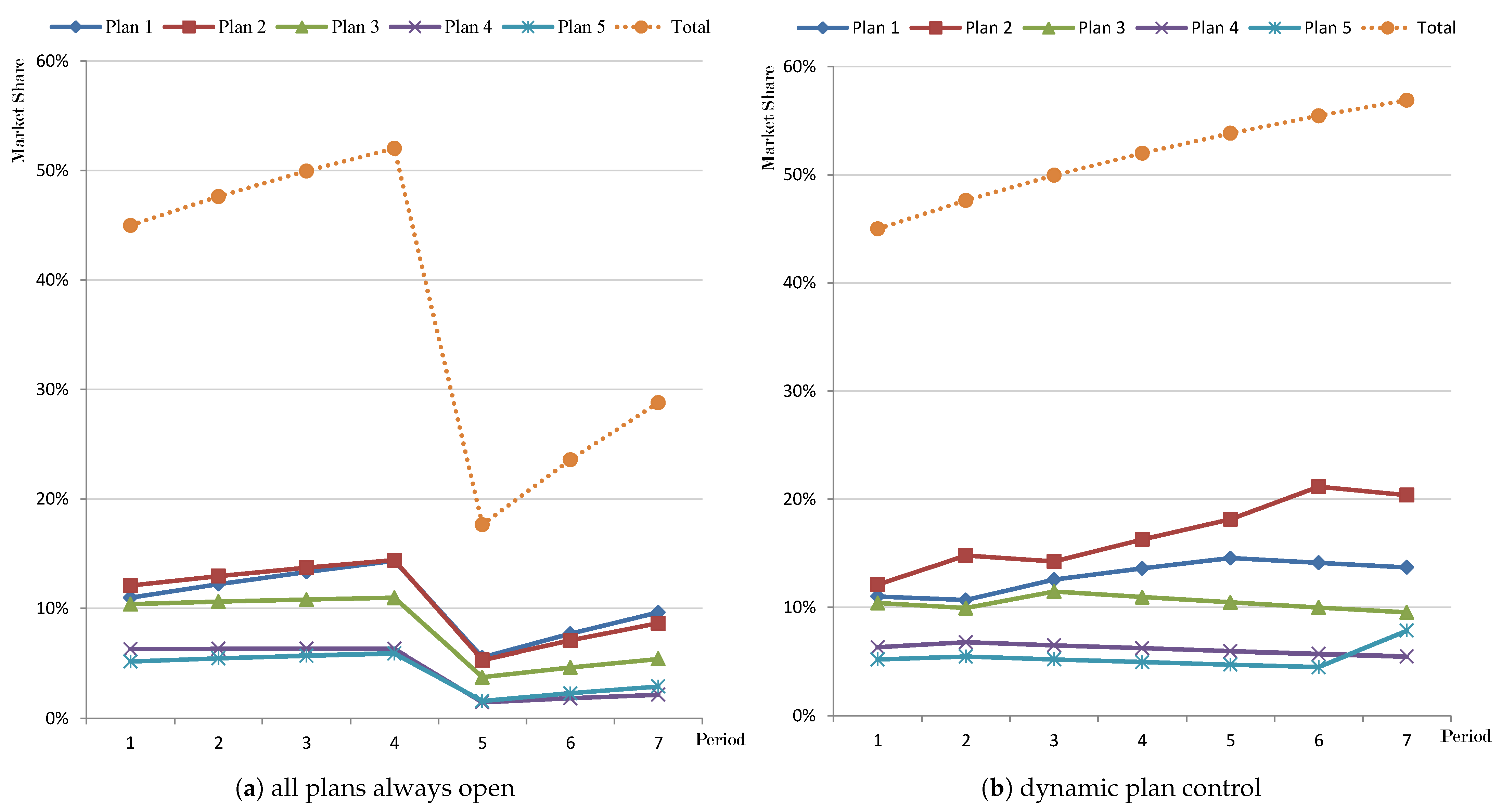
Our study has three contributions. First, we take the limited network capacity into consideration and build a dynamic plan control model. The traditional dynamic pricing of mobile data plans focuses on finding the optimal pricing parameters by assuming that network capacity is unlimited. However, with the rapid growth of data traffic, network capacity has become a bottleneck that affects how service providers can address customers’ demand. This research attempts to offer new insights into managing demand when network capacity is limited. Compared with the all plans always open method, which is currently implemented by most mobile service providers, our dynamic plan control method can dynamically open a subset of data plans for new customers at the beginning of each period. This dynamic control allows the service provider to adjust data network utilization and achieve high customer satisfaction and a low churn rate, which reflect high service supply chain performance.

Second, we provide a framework to model the behaviors of service providers and customers under connection-speed-restriction pricing. Despite the growing popularity of connection-speed-restriction pricing, little research has been devoted to demand management under this pricing scheme. Our study addresses this issue and models the behaviors of both service providers and customers under connection-speed-restriction pricing.

Third, the service provider’s optimization problem is a dynamic programming problem. Due to the high-dimensional property of the problem, it is difficult to implement backward induction. To solve the problem efficiently, we propose an equivalent mixed integer linear programming (MILP) formulation. Through numerical evaluation, the efficiency of the solution method is further validated.

The remainder of this paper is organized as follows. We conduct a brief review of the relevant literature in Section 2. In Section 3, we describe the models of the service provider and customers. Section 4 provides the solution approach, and Section 5 examines the effect of our model with numerical experiments. Finally, Section 6 offers some concluding remarks and future research directions.

2. Literature Review

Our research relates to two topics in the literature: the pricing scheme used for mobile data service and the demand management methods considering congestion used by mobile service providers. In this section, we review the relevant works on these two topics.

2.1. Pricing Scheme

The pricing scheme used for mobile data service has evolved in the past two decades. Because flat-rate pricing is easy to implement and quite effective in stimulating data demand [10], it was popular when the total market demand for data service was low. As data demand grew, mobile service providers moved to metered pricing, where a customer is charged a fixed fee first and then a per-unit fee. In contrast to flat-rate pricing, metered pricing allows mobile service providers to facilitate price discrimination and thereby increase their revenue [11,12]. In practice, there are two versions of metered pricing: two part pricing and three part pricing. The difference is that three part pricing bundles some allotted data into the fixed fee, but two part pricing does not (see Figure 1a,b). Danaher [13] studied two part pricing and found the optimal fixed fee and per-unit fee for the revenue-maximizing strategy. In addition, they showed that the fixed fee and per-unit fee have different relative effects on the demand and retention of users.

A similar investigation analyzed three part pricing. Reference [14] assumed that each consumer has a predetermined demand. He showed that for consumers who are not overconfident, the firm’s optimal strategy is a high fixed fee and thus takes all of the consumers’ surplus. Furthermore, the firm’s profit increases if the consumers are overconfident. Later, Reference [15] characterized the optimal three part pricing plan under more general conditions. Based on a global bound for the service provider’s profit, they employed a methodology that was different from the standard first-order conditions approach and showed that this bound is attained using the optimal plan. In addition, some researchers compared two part pricing and three part pricing and tried to find which one was better for service providers. Reference [12] concluded that a relatively small menu of three part pricing can be more profitable than a menu of two part pricing of any size. In contrast, Reference [16] showed that the optimal three part pricing outcomes are identical to the optimal two part pricing outcomes when the market demand follows an increasing price elasticity or when the consumer distribution approximately follows an increasing hazard rate.

Since we entered the era of 4G, connection-speed-restriction pricing has rapidly become a popular pricing scheme used by the industry. Figure 1 shows the differences among two part pricing, three part pricing, and connection-speed-restriction pricing. In an overview of smart data pricing, Sen et al. [17] addressed connection-speed-restriction pricing as a new trend of data pricing. However, to the best of our knowledge, few studies have been devoted to connection-speed-restriction pricing. Our study aims to fill this gap.

2.2. Demand Management Considering Congestion

Another relevant stream of the literature is demand management methods considering congestion in mobile Internet networks. As the demand for data service grew dramatically, demand management has become a new challenge for service providers. Research on demand management is conducted mainly considering two concepts, time-dependent pricing and the traffic offloading mechanism, which aim to relieve network congestion by giving users incentives to shift their mobile data demand to less-congested time periods or to supplementary networks (such as Wi-Fi) [18].

Time-dependent pricing has many variants. The most basic version is time-of-day pricing, which charges users a higher price for data usage during certain “peak” hours of the day than at other times of the day, so that network congestion in these time periods can be relieved [19,20,21]. In contrast to time-of-day pricing, day-ahead pricing computes new prices for different times of the next day in advance, based on predicted congestion levels. Reference [22] showed that day-ahead pricing benefits both service providers and customers, flattening the temporal fluctuation of data demand while allowing users to save money by choosing the time and volume of their usage. Besides, day-ahead pricing is also used in the electricity pricing context. Reference [23] considered a model for a single smart home and for a community (multiple homes) with different priorities. The priority was assigned to each appliance by electricity consumers. In their scheme, day-ahead real time pricing (DA-RTP) and critical peak pricing (CPP) were utilized to calculate electricity cost. Time-dependent pricing typically requires information about user demand [24,25]. To obtain a reliable forecast of user demand, Reference [26] built a multiple equation time-series model. For day-ahead forecasting, the mean absolute percentage error (MAPE) returned by the model over a period of 11 years was an impressive 1.36%, which is superior to all benchmarks that the authors chose.

In addition to time-dependent pricing, service providers can manage demand by encouraging users to shift some of their data traffic to supplementary networks such as Wi-Fi [27]. Reference [28] noted that the success of such a “traffic offloading” strategy largely relies on the economic incentives provided to users. Reference [29] proposed a novel congestion-optimal Wi-Fi offloading (COWO) algorithm based on the subgradient method, which aims to obtain the optimal offloading ratio for each access point to maximize the throughput and minimize network congestion. Reference [30] proposed a downloading mechanism in different vehicular networks that comprises an ad hoc network and a cellular network. In this mechanism, roadside units act as traffic managers to collect data from the Internet and then distribute them to vehicles in an approximately optimal manner. Reference [31] constructed an intelligent offloading method for vehicular networks. They jointly utilized licensed cellular spectrum and unlicensed channels and used the real data of the traces of taxies to illustrate the effectiveness of the solution. In general, Reference [18] stated that the realizations of time-dependent pricing and traffic offloading can help create a financial win-win solution for service providers and their users.

Although time-dependent pricing and traffic offloading mechanisms have been proven to be helpful in demand management, they have some drawbacks and limitations [18,32]. Time-dependent pricing makes the price change too frequently, which leads to extra costs, including operational costs and costs to help consumers in understanding and making a selection from a complex menu of choices [33]. Traffic offloading seems to be the direction in which many service providers are going today, but it requires investment in expanding wired and wireless network capacities.

To meet these challenges, we propose another demand management tool, the dynamic plan control method, which can dynamically control open and closed plans for potential customers in each period to relieve mobile network congestion. Moreover, we innovatively apply it in the framework of connection-speed-restriction pricing, which is increasingly popular now that 4G and 5G are available.

3. The Model

A mobile service provider (SP) employs connection-speed-restriction pricing and offers m different data plans. The information about the data plans is pre-announced to the customers. We consider a market composed of a large number of customers. The customer population, denoted by N, is deterministic.

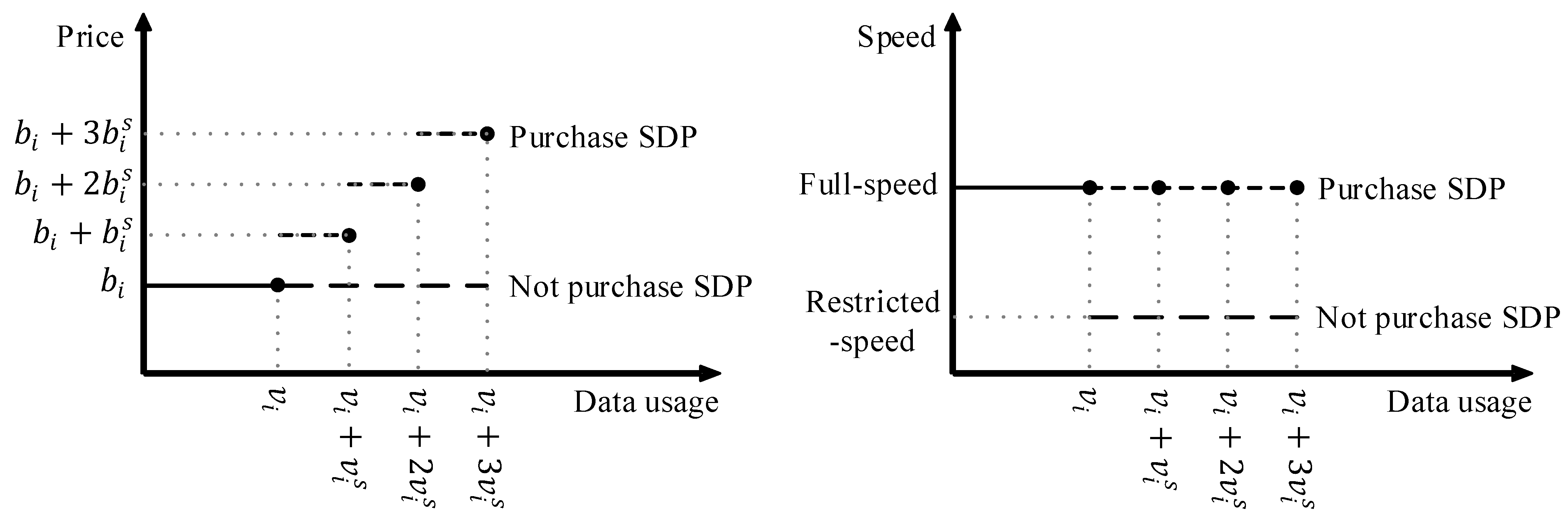
All data plans give customers unlimited data. The differences between the data plans are their prices and allotted volumes of full-speed data. We denote $b_i$ as the price per period of data plan i and $v_i$ as the allotted volume of full-speed data in data plan i. To use the data service, a customer needs to subscribe to a data plan first. Connection-speed-restriction pricing implies that for a customer subscribed to data plan i, his/her individual data speed will be restricted after he/she uses up the allotted volume of full-speed data $v_i$ in his/her data plan. If the customer wants to re-obtain full-speed data connection, he/she needs to buy the supplementary data package or wait until the beginning of the next period.

The supplementary data package (SDP) provides the customers with additional full-speed data. In addition, the purchase of the supplementary data package can be performed repeatedly as desired. According to the SP’s arrangement, different data plans may offer different supplementary data packages. A customer can only buy the supplementary data package that is attached to his/her data plan. In this paper, we consider the situation in which each data plan offers only one type of supplementary data package. For the ease of exposition, we address the supplementary data package attached to data plan i as “supplementary data package i”. We denote $b_i^s$ as the price per purchase of supplementary data package i and $v_i^s$ as the additional volume of full-speed data within supplementary data package i. For example, if a customer subscribes to data plan i and wants to consume data volume $v_i+3v_i^s$ at full speed in one period, then she/he needs to buy supplementary data package i three times, and her/his total cost in this period is $b_i+3b_i^s$.

An overview of the data plan parameters is given in

Table 1. Parameters of the data plan and supplementary data package (SDP).

Data plan i	${\mathit{v}}_{\mathit{i}}$	=	The allotted volume of full-speed data within data plan i
	$b_i$	=	The price per period of data plan i
Supplementary data package i	$v_i^s$	=	The additional volume of full-speed data gained by purchasing supplementary data package i
	$b_i^s$	=	The price per purchase of supplementary data package i

, and the mechanism of connection-speed-restriction pricing is illustrated in Figure 2.

For the ease of discussion, we sort all data plans by price; that is, $b_1<\cdots <b_i<\cdots <b_m$. Then, the allotted volumes of full-speed data within all data plans satisfy $v_1<\cdots <v_i<\cdots <v_m$. In addition, we make the following assumptions.

Assumption. 

For all data plans and supplementary data packages, we have:

1. 

${\displaystyle \frac{b_1}{v_1}}\ge \cdots \ge {\displaystyle \frac{b_i}{v_i}}\ge \cdots \ge {\displaystyle \frac{b_m}{v_m}}$,

2. 

${\displaystyle \frac{b_1^s}{v_1^s}}\ge \cdots \ge {\displaystyle \frac{b_i^s}{v_i^s}}\ge \cdots \ge {\displaystyle \frac{b_m^s}{v_m^s}}$,

3. 

$b_{i+1}<b_i+⌈{\displaystyle \frac{v_{i+1}-v_i}{v_i^s}}⌉·b_i^s,\forall i=1,2,\cdots ,m-1$.

These three assumptions are mild and easily satisfied in real practice. Assumptions 1 and 2 are straightforward: a high-priced data plan (and its corresponding supplementary data package) means a low unit price of full-speed data. Assumption 3 implies that when a customer’s full-speed data usage is larger than a critical value, a higher price data plan is always preferred by the customer over a lower price data plan.

Because the network capacity is fixed, network congestion occurs when the overall data traffic in the network exceeds a threshold. Network congestion influences the customer experience, resulting in a number of customers leaving the network. To manage network congestion, the service provider can use the dynamic plan control method. With this method, the service provider opens a subset of data plans in each period, and potential customers can subscribe to only the open data plans. Let $C_{i,t}$ be a binary variable indicating the open/closed status of the data plan i in period t. $C_{i,t}=1$ if the data plan i is open in period t, and $C_{i,t}=0$ otherwise. In the following, we model the behaviors of the service provider and customers and then give the service provider’s revenue function.

3.1. Decisions of Potential Customers

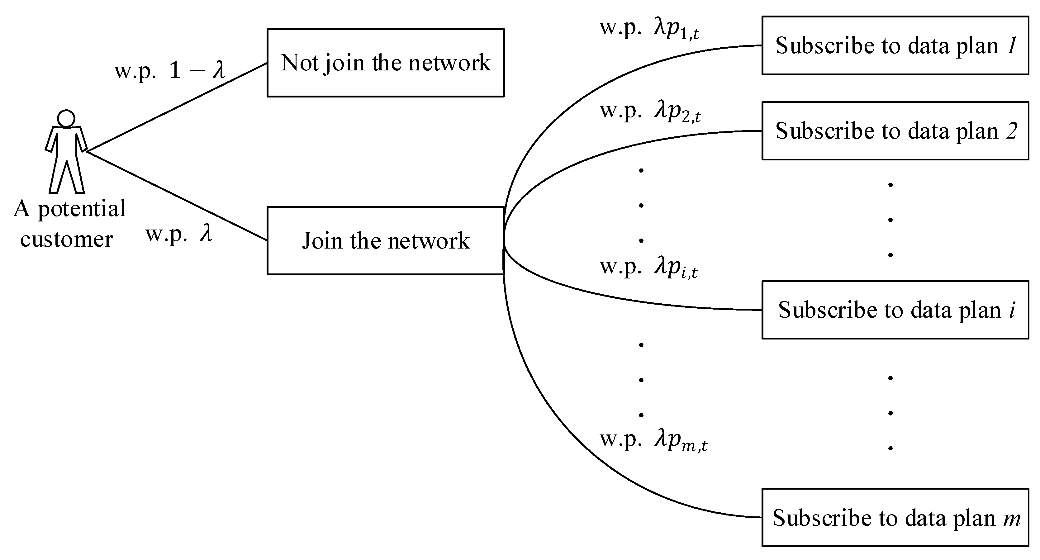
Potential customers are those who are not in the service provider’s network. In each period, a potential customer decides whether to join the service provider’s network first and then chooses a data plan from all open data plans. As illustrated in Figure 3, the decision process is investigated in two stages. In Stage 1, the probability that a potential customer joins the network, denoted by $\lambda$, reflects the potential customer’s willingness to join the network. This willingness is influenced by the service provider’s reputation and advertising rather than the dynamic plan control. To avoid unnecessary complexity, we let $\lambda$ be exogenous and constant over periods. In Stage 2, we denote $p_{i,t}$ as the probability that a potential customer subscribes to data plan i in period t. By definition, we have ${\sum }_{i=1}^m{p}_{i,t}=1$.

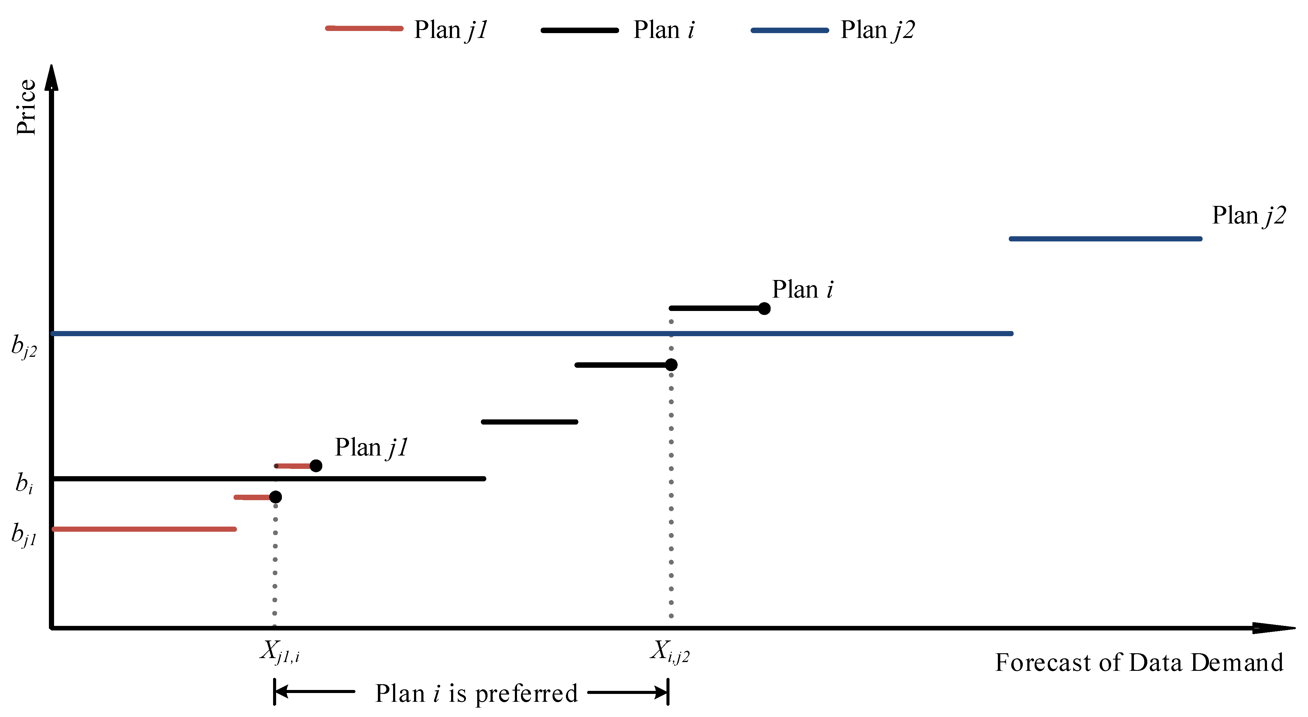
In Stage 2, a potential customer chooses a data plan based on his/her forecast of data demand. Let $\widehat{D}$ be the potential customer’s forecast of data demand in a single period. The potential customers’ demand forecasts are heterogeneous and distributed independently and identically with a cumulative distribution function $F\left(\widehat{D}\right)$, which is common knowledge to both the service provider and customers. For a potential customer with demand forecast $\widehat{D}$, we denote $r_i\left(\widehat{D}\right)$ as the cost for using data service at full speed in a single period if she/he subscribes to data plan i. Then, we have:

$$r_i\left(\widehat{D}\right)=b_i+⌈\frac{{(\widehat{D}-v_i)}^{+}}{v_i^s}⌉·b_i^s.$$

When deciding which data plan to choose in Stage 2, the potential customers are concerned about both speed and cost. They choose the data plan that provides full-speed data service with minimal cost in all open plans. Therefore, $p_{i,t}$ can be formulated as:

$$p_{i,t}=\mathrm{Pr}\left(C_{i,t}=1,r_i\left(\widehat{D}\right)\le \underset{j:C_{j,t}=1}{min}{r}_j\left(\widehat{D}\right)\right).$$

3.2. Characteristics of the Subscribed Customers

For a customer subscribed to data plan i, we introduce a vector $(U_i,U_i^f)$, where $U_i$ is his/her total data usage (including full-speed data usage and restricted-speed data usage) in a period and $U_i^f$ is his/her full-speed data usage in a period. In each period, the subscribed customer consumes data continuously throughout the entire period. Therefore, the vector $(U_i,U_i^f)$ is random at the beginning of the period and realized at the end of the period.

We model two key characteristics of the subscribed customers’ behavior. First, a customer’s total data usage does not necessarily equal her/his data demand forecast, despite the fact that the customer chooses the data plan based on her/his data demand forecast. Generally, the customer’s total data usage fluctuates around the volume of full-speed data in her/his data plan. This is reasonable because if the customer’s total data usage is far below $v_i$, then she/he should have subscribed to a “low-priced” data plan. If the customer’s total data usage is far beyond $v_i$, then she/he should have subscribed to a “high-priced” data plan. Therefore, we assume that the expected volume of the customer’s total data usage equals the volume of full-speed data in her/his data plan; that is, $\mathbb{E}\left[U_i\right]=v_i$. In addition, we assume that the total data usage of all customers subscribed to plan i are distributed independently and identically with a cumulative distribution function $F_i\left(U_i\right)$. Moreover, $F_i\left(U_i\right)$ is homogeneous over periods.

Second, if a subscribed customer wants to consume more full-speed data than the allotted volume within his/her data plan, he/she purchases the supplementary data package repeatedly to maintain full speed throughout the entire period. This assumption is reasonable because the marginal price for any supplementary data package is constant.

We can classify the subscribed customers of data plan i into three categories: A, B, and C. For a customer of category A, her/his total data usage does not exceed the allotted full-speed data $v_i$. For a customer of category B, the total data usage exceeds $v_i$, but he/she does not purchase the supplementary data package. For a customer of category C, the total data usage exceeds $v_i$, and she/he purchases the supplementary data package i repeatedly. The customers of category A and category C use data at full speed throughout the entire period. However, the customers of category B use the restricted-speed data service, which leads to customer dissatisfaction. An overview of the three categories is given in

Table 2. Three categories of subscribed customers.

	Total Data Usage ${\mathit{U}}_{\mathit{i}}$	Willing to Buy SDP	Full-Speed Data Usage ${\mathit{U}}_{\mathit{i}}^{\mathit{f}}$	Price to Pay in One Period	Customer Satisfaction
Category A	$\le v_i$	Not necessary	$=U_i$	$=b_i$	Yes
Category B	$>v_i$	No	$=v_i$	$=b_i$	No
Category C	$>v_i$	Yes	$=U_i$	$=b_i+k·b_i^s$	Yes

.

Let $S_{i,t}$ be the number of customers subscribed to data plan i at the beginning of period t. Let $S_{i,t}^A$, $S_{i,t}^B$, and $S_{i,t}^C$ be the number of customers in the A, B, and C categories, respectively. By definition, we have $S_{i,t}=S_{i,t}^A+S_{i,t}^B+S_{i,t}^C$. In addition, we define $w_i=S_{i,t}^C/(S_{i,t}^B+S_{i,t}^C)$, which reflects the customers’ willingness to purchase supplementary data packages. We assume that $w_i$ is constant over periods.

In period t, the customers of both A and B categories pay $b_i$. The service provider’s revenue generated from the customers of category A and category B is:

$$\sum _{i=1}^m(S_{i,t}^A+S_{i,t}^B)·b_i.$$

To formulate the revenue generated from the customers of category C, we need to further differentiate the data usage. We define k ($k\in {\mathbb{N}}^{+}$) as an integer that satisfies $v_i+(k-1)·v_i^s<U_i\le v_i+k·v_i^s$, where k denotes the number of supplementary data packages a category C customer with data usage $U_i$ purchases in a single period. Let $S_{i,t}^{C,k}$ be the number of subscribed customers of data plan i who purchase k supplementary data packages in period t. Then, the service provider’s revenue generated from the customers of category C in period t is:

$$\sum _{i=1}^m\sum _{k=1}^{k_t^{*}}{S}_{i,t}^{C,k}·(b_i+k·b_i^s),$$

where $k_t^{*}$ denotes the largest k in period t.

3.3. Network Congestion and Plan-Leaving Characteristics

Network congestion occurs when total full-speed data usage exceeds a threshold. Let $G_t$ be a binary variable indicating whether network congestion occurs in period t. $G_t=1$ if network congestion occurs in periods t, and $G_t=0$ if not.

For a subscribed customer of data plan i, the expected volume of full-speed data usage in a single period is $\mathbb{E}\left[U_i^f\right]$. By definition, we have:

$$\mathbb{E}[U_i^f]={\int }_0^{v_i}{U}_i·f_i\left(U_i\right)\mathrm{d}{U}_i+v_i·[1-F_i\left(v_i\right)]·(1-w_i)+{\int }_{v_i}^{\infty }{U}_i·f_i\left(U_i\right)·w_i\mathrm{d}{U}_i.$$

When the subscribed customers feel unsatisfied with the service, they may quit the service. There are multiple reasons that lead to customer dissatisfaction, but we model only the two most important reasons, namely network congestion (NC) and individual speed restriction (ISR). Let $q_{i,t}^P$ be the probability that a customer quits the service when NC happens but ISR does not and $q_{i,t}^E$ be the probability that a customer quits the service when ISR happens, but NC does not.

Let $q_{i,t}$ be the probability that a subscribed customer quits the service. Because network congestion and individual speed restriction are two independent events, we have:

$$q_{i,t}=\left\{\begin{array}{cc}{\overline{F}}_i\left(v_i\right)(1-w_i)q_{i,t}^E\hfill & ,\mathrm{if}\mathrm{NC}\mathrm{does}\mathrm{not}\mathrm{happen}\mathrm{in}\mathrm{period}\mathrm{t}\hfill \\ q_{i,t}^P+[{\overline{F}}_i\left(v_i\right)(1-w_i)q_{i,t}^E]-q_{i,t}^P·[{\overline{F}}_i\left(v_i\right)(1-w_i)q_{i,t}^E]\hfill & ,\mathrm{if}\mathrm{NC}\mathrm{happens}\mathrm{in}\mathrm{period}\mathrm{t}\hfill \end{array}\right.$$

(1)

3.4. Dynamic Programming Formulation

We consider a total of T periods. In period t, the population size of potential customers is $N-{\sum }_{i=1}^m{S}_{i,t}$. Each potential customer either subscribes to a data plan or does not join the network. Let $Y_{i,t}$ be the number of new customers subscribing to data plan i in period t. Therefore, we can build a multinomial distribution model for $Y_t=(Y_{1,t},\cdots ,Y_{m,t})$; that is, $Y_t\sim \mathrm{PN}(N-{\sum }_{i=1}^m{S}_{i,t}:\lambda p_{1,t},\cdots ,\lambda p_{m,t})$. For all $0\le {\sum }_{i=1}^m{y}_{i,t}\le N-{\sum }_{i=1}^m{S}_{i,t}$, we have the probability mass function:

$$\begin{array}{ccc}\hfill \mathrm{Pr}\left(Y_t=y_t\right)& =& \mathrm{Pr}\left(Y_{1,t}=y_{1,t},\cdots ,Y_{m,t}=y_{m,t}\right)\hfill \\ & =& {\displaystyle \frac{(N-{\displaystyle \sum _{i=1}^m}{S}_{i,t})!{(1-\lambda )}^{(N-{\displaystyle \sum _{i=1}^m}{S}_{i,t}-{\displaystyle \sum _{i=1}^m}{y}_{i,t})}{\left(\lambda p_{1,t}\right)}^{y_{1,t}}\cdots {\left(\lambda p_{m,t}\right)}^{y_{m,t}}}{(N-{\displaystyle \sum _{i=1}^m}{S}_{i,t}-{\displaystyle \sum _{i=1}^m}{y}_{i,t})!\left(y_{1,t}\right)!\cdots \left(y_{m,t}\right)!}}.\hfill \end{array}$$

Similar to the classification we employ for subscribed customers, we classify new customers into three categories and denote $Y_{i,t}^A$, $Y_{i,t}^B$, and $Y_{i,t}^C$ as the number of new customers in the A, B, and C categories, respectively. In addition, we assume that $Y_{i,t}^C/(Y_{i,t}^B+Y_{i,t}^C)=w_i$. The willingness to purchase supplementary data packages is heterogeneous for customers with different data plans, but homogeneous for old customers and new customers.

Let $L_{i,t}$ be the number of customers quitting plan i at the end of period t. A subscribed customer either does not quit the service or quits the service at the end of period. Therefore, we can build a binomial distribution model for $L_t=(L_{1,t},\cdots ,L_{m,t})$; that is, $L_{i,t}\sim \mathrm{B}(S_{i,t},q_{i,t})$. For all $0\le l_{i,t}\le S_{i,t}$, we have the probability mass function:

$$\begin{array}{ccc}\hfill \mathrm{Pr}\left(L_t=l_t\right)& =& \mathrm{Pr}\left(L_{1,t}=l_{1,t}\right)·\cdots ·\mathrm{Pr}\left(L_{m,t}=l_{m,t}\right)\hfill \\ & =& \prod _{i=1}^m\frac{S_{i,t}!}{l_{i,t}!(S_{i,t}-l_{i,t})!}{\left(q_{i,t}\right)}^{l_{i,t}}{(1-q_{i,t})}^{S_{i,t}-l_{i,t}}.\hfill \end{array}$$

Let $V_t\left(S_t\right)$ be the service provider’s maximum revenue from period t to the end, starting at state $S_t=(S_{1,t},\cdots ,S_{m,t})$ at the beginning of period t. The dynamic programming problem, which is to maximize $V_t\left(S_t\right)$ by choosing the right $C_{i,t}$, can be written as follows:

$$\begin{array}{ccc}\hfill \left(\mathbf{DP}\mathbf{1}\right)& & V_t\left(S_t\right)\hfill \\ & =& \sum _{i=1}^m\left(\mathbb{E}\left[S_{i,t}^A\right]+\mathbb{E}\left[S_{i,t}^B\right]\right)·b_i+\sum _{i=1}^m\sum _{k=1}^{k^{*}}\mathbb{E}\left[S_{i,t}^{C,k}\right]·(b_i+k·b_i^s)\hfill \\ & & +\underset{C_t\in {\left\{0,1\right\}}^m}{max}\left\{\sum _{i=1}^m\left(\mathbb{E}\left[Y_{i,t}^A\right]+\mathbb{E}\left[Y_{i,t}^B\right]\right)·b_i+\sum _{i=1}^m\sum _{k=1}^{k^{*}}\mathbb{E}\left[Y_{i,t}^{C,k}\right]·\left(b_i+k·b_i^s\right)+\mathbb{E}\left[V_{t+1}\left(S_{t+1}\right)\right]\right\},\forall t.\hfill \end{array}$$

The transition function is $S_{t+1}=S_t+Y_t-L_t$, and the boundary conditions are $V_{T+1}\left(S_{T+1}\right)=0$ for all $S_{T+1}$.

4. Solution

4.1. Formulation of the Continuous State Problem

The service provider’s optimization problem is a dynamic programming problem with discrete states. In practice, the customer population N is so large that the traditional backward induction solution is hard to implement. For this reason, we proceed to analyze the continuous state problem in limiting case $N\to +\infty$.

To characterize the percentage of customers already in data plan i at the beginning of period t, we define ${\theta }_{i,t}=\underset{N\to +\infty }{lim}{S}_{i,t}/N$. For convenience, we define ${\theta }_{0,t}=\underset{N\to +\infty }{lim}(N-{\sum }_{i=1}^m{S}_{i,t})/N$. Moreover, we let ${\overline{V}}_t\left({\mathit{\theta }}_t\right)$ be the service provider’s maximum average revenue per customer from period t to the end, starting at state ${\mathit{\theta }}_t=({\mathit{\theta }}_{0,t},{\mathit{\theta }}_{1,t},\cdots ,{\mathit{\theta }}_{m,t})$. To simplify the expression, we let:

$${\rho }_i=\sum _{k=1}^{k_t^{*}}\left[F_i\left(v_i+k{v}_i^s\right)-F_i\left(v_i+\left(k-1\right)v_i^s\right)\right]·(1+k·{\displaystyle \frac{b_i^s}{b_i}}),$$

where ${\rho }_i$ can be interpreted as the expectation that a customer of category C has to pay more than customers of category A or B.

The dynamic programming problem (DP2) can be written as follows:

$$\begin{array}{ccc}\hfill \left(\mathbf{DP}\mathbf{2}\right)& & {\overline{V}}_t\left({\theta }_t\right)\hfill \\ & =& \sum _{i=1}^m{\theta }_{i,t}·\left[F_i\left(v_i\right)+{\overline{F}}_i\left(v_i\right)·(1-w_i)+{\rho }_i·w_i\right]·b_i\hfill \\ & & +\underset{C_t\in {\left\{0,1\right\}}^m}{max}\left\{{\theta }_{0,t}·\sum _{i=1}^m\lambda p_{i,t}·\left[F_i\left(v_i\right)+{\overline{F}}_i\left(v_i\right)·(1-w_i)+{\rho }_i·w_i\right]·b_i+\mathbb{E}\left[{\overline{V}}_{t+1}(A_t({\theta }_t,I_t)·{\theta }_t)\right]\right\},\forall t.\hfill \end{array}$$

The boundary conditions are ${\overline{V}}_{T+1}\left({\theta }_{T+1}\right)=0$ for all ${\theta }_{T+1}$. The transition matrix $A_t({\mathit{\theta }}_t,C_t)$ can be formulated as:

$${\mathit{A}}_{\mathit{t}}\mathbf{(}{\mathit{\theta }}_{\mathit{t}},{\mathit{C}}_{\mathit{t}}\mathbf{)}=\left[\begin{array}{cc}{\mathit{A}}_{\mathbf{1}}& {\mathit{A}}_{\mathbf{2}}\\ {\mathit{A}}_{\mathbf{3}}& {\mathit{A}}_{\mathbf{4}}\end{array}\right],$$

where $A_1\in \mathbb{R}$, $A_2\in {\mathbb{R}}^{1\times m}$, $A_3\in {\mathbb{R}}^{m\times 1}$, and $A_4\in {\mathbb{R}}^{m\times m}$ with:

$$\begin{array}{ccc}& & A_1=1-\sum _{i=1}^m\lambda ·p_{i,t},\hfill \\ & & {\left\{A_2\right\}}_i=\lambda ·p_{i,t},\forall i,\hfill \\ & & {\left\{A_3\right\}}_{\tilde{i}}=q_{\tilde{i},t},\forall \tilde{i},\hfill \\ & & {\left\{A_4\right\}}_{i\tilde{i}}=\left\{\begin{array}{c}1-q_{i,t},\mathrm{if}i=\tilde{i},\forall i,\tilde{i},\hfill \\ 0,\mathrm{if}i\ne \tilde{i},\forall i,\tilde{i}.\hfill \end{array}\right.\hfill \end{array}$$

According to the definition of ${\theta }_{i,t}$, we have:

$$\begin{array}{c}{\sum }_{i=1}^m{\theta }_{i,t}·\left[F_i\left(v_i\right)+\overline{F_i}\left(v_i\right)(1-w_i)+{\rho }_i·w_i\right]·b_i\\ ={\sum }_{i=1}^m\underset{N\to \infty }{lim}\frac{S_{i,t}}{N}·\left[F_i\left(v_i\right)+\overline{F_i}\left(v_i\right)(1-w_i)+{\rho }_i·w_i\right]·b_i\\ =\underset{N\to \infty }{lim}\frac{1}{N}\left\{{\sum }_{i=1}^m\left[S_{i,t}{F}_i\left(v_i\right)+S_{i,t}\overline{F_i}\left(v_i\right)(1-w_i)\right]·b_i\right.\\ +\left.{\sum }_{i=1}^m{S}_{i,t}·{\sum }_{k=1}^{k_t^{*}}\left[F_i\left(v_i+k{v}_i^s\right)-F_i\left(v_i+\left(k-1\right)v_i^s\right)\right]·(b_i+k·b_i^s)\right\}\\ =\underset{N\to \infty }{lim}\frac{1}{N}\left\{{\sum }_{i=1}^m\left(\mathbb{E}\left[S_{i,t}^A\right]+\mathbb{E}\left[S_{i,t}^B\right]\right)·b_i+{\sum }_{i=1}^m{\sum }_{k=1}^{k_t^{*}}\mathbb{E}\left[S_{i,t}^{C,k}\right]·(b_i+k·b_i^s)\right\},\forall t.\end{array}$$

(2)

Analogously, we can derive:

$$\begin{array}{cc}\hfill & \underset{C_t\in {\left\{0,1\right\}}^m}{max}\left\{{\theta }_{0,t}{\sum }_{i=1}^m\lambda ·p_{i,t}·\left[F_i\left(v_i\right)+\overline{F_i}\left(v_i\right)(1-w_i)+{\rho }_i·w_i\right]·b_i\right\}\\ \hfill =& \underset{N\to \infty }{lim}\frac{1}{N}\underset{C_t\in {\left\{0,1\right\}}^m}{max}\left\{{\sum }_{i=1}^m\left(\mathbb{E}\left[Y_{i,t}^A\right]+\mathbb{E}\left[Y_{i,t}^B\right]\right)·b_i+{\sum }_{i=1}^m{\sum }_{k=1}^{k_t^{*}}\mathbb{E}\left[Y_{i,t}^{C,k}\right]·\left(b_i+k·b_i^s\right)\right\},\forall t.\end{array}$$

(3)

Summing (2) and (3) over t and plugging them into the formulation of Data Plan 2 (DP2), we obtain:

$${\overline{V}}_t\left({\mathit{\theta }}_t\right)=\underset{N\to \infty }{lim}\frac{V_t\left(S_t\right)}{N},\forall t.$$

Due to the strong law of large numbers, we can reformulate ${\theta }_{i,t+1}$ and ${\theta }_{0,t+1}$ as follows.

$$\begin{array}{ccc}\hfill {\theta }_{i,t+1}& =& \underset{N\to \infty }{lim}\frac{S_{i,t+1}}{N}\hfill \\ & =& \underset{N\to \infty }{lim}\frac{S_{i,t}+Y_{i,t}-L_{i,t}}{N}\hfill \\ & =& {\theta }_{0,t}·\lambda p_{i,t}+{\theta }_{i,t}·(1-q_{i,t}),\forall i,t.\hfill \end{array}$$

(4)

$$\begin{array}{ccc}{\theta }_{0,t+1}& =& 1-\sum _{i=1}^m{\theta }_{i,t+1}\hfill \\ & =& 1-\sum _{i=1}^m\left\{{\theta }_{0,t}·\lambda p_{i,t}+{\theta }_{i,t}·(1-q_{i,t})\right\}\hfill \\ & =& {\theta }_{0,t}·(1-\sum _{i=1}^m\lambda p_{i,t})+\sum _{i=1}^m{\theta }_{i,t}·q_{i,t},\forall t.\hfill \end{array}$$

(5)

Combining (4) and (5), we have the transition function ${\theta }_{t+1}=A_t({\theta }_t,C_t)·{\theta }_t.$

The arguments above can be summarized in the following theorem.

Theorem 1.

The optimal objective value in (DP2) equals the optimal objective value in (DP1): ${\overline{V}}_1\left({\theta }_1\right)=\underset{N\to \infty }{lim}{V}_1\left(S_1\right)/N$.

Theorem 1 suggests that when the customer population becomes large enough (which is easily satisfied in real applications), we can approximately solve the SP’s dynamic programming problem with discrete states by solving a related problem with a continuous state.

4.2. Formulation of Mixed Integer Linear Programming

In this subsection, an equivalent mixed integer linear programming (MILP) formulation is proposed. With this MILP formulation, we can solve the dynamic programming problem with a continuous state much more efficiently.

4.2.1. System state transitions

Define ${\alpha }_{i,t}={\theta }_{0,t}·\lambda p_{i,t}$ and ${\beta }_{i,t}={\theta }_{i,t}·q_{i,t}$, where ${\alpha }_{i,t}$ denotes the percentage of new customers who join plan i in period t and ${\beta }_{i,t}$ denotes the percentage of customers quitting plan i in period t. Then, we have the following state transition functions:

$$\begin{array}{cc}\hfill & {\theta }_{i,t+1}={\theta }_{i,t}+{\alpha }_{i,t}-{\beta }_{i,t},\forall i,t,\hfill \\ \hfill & {\theta }_{0,t+1}={\theta }_{0,t}-\sum _{i=1}^m{\alpha }_{i,t}+\sum _{i=1}^m{\beta }_{i,t},\forall t,\hfill \\ \hfill & \sum _{i=0}^m{\theta }_{i,t}=1.\hfill \end{array}$$

(6)

4.2.2. Percentage of New Customers

Figure 4 shows how we determine the probability $p_{i,t}$. For all open data plans i, $j1$, and $j2$ that satisfy $1\le j1<i<j2\le m$, a potential customer chooses a data plan i if her/his data demand forecast falls into the interval $(X_{j1,i},X_{i,j2}]$, where:

$$X_{j1,i}=v_{j1}+⌊{\displaystyle \frac{b_i-b_{j1}}{b_{j1}^s}}⌋·v_{j1}^s,X_{i,j2}=v_i+⌊{\displaystyle \frac{b_{j2}-b_i}{b_i^s}}⌋·v_i^s.$$

Conventionally, we can determine $p_{i,t}$ by a list of constraints first and then determine ${\alpha }_{i,t}$ by the relationship between $p_{i,t}$ and ${\alpha }_{i,t}$. However, in the definition of ${\alpha }_{i,t}$, the term ${\theta }_{0,t}·p_{i,t}$ is not a linear term, so we determine ${\alpha }_{i,t}$ directly by the following constraints:

$$\begin{array}{cc}\hfill & {\alpha }_{i,t}\le M·C_{i,t},\forall i,t,\hfill \\ \hfill & {\alpha }_{i,t}\le {\theta }_{0,t}·\lambda \left[F\left(X_{i,j2}\right)-F\left(X_{j1,i}\right)\right]+M\left(2-C_{j1,t}-C_{j2,t}\right),\forall 1\le j1<i<j2\le m,\forall t,\hfill \\ \hfill & {\alpha }_{i,t}\le {\theta }_{0,t}·\lambda \left[F\left(X_{i,j2}\right)-F\left(X_{0,i}\right)\right]+M\left(1-C_{j2,t}\right),\forall 1\le i<j2\le m,\forall t,\hfill \\ \hfill & {\alpha }_{i,t}\le {\theta }_{0,t}·\lambda \left[1-F\left(X_{j1,i}\right)\right]+M\left(1-C_{j1,t}\right),\forall 1\le j1<i\le m,\forall t,\hfill \\ \hfill & {\alpha }_{i,t}\le {\theta }_{0,t}·\lambda \left[1-F\left(X_{0,i}\right)\right],\forall i,t,\hfill \\ \hfill & \sum _{i=1}^m{\alpha }_{i,t}={\theta }_{0,t}·\lambda ,\forall t.\hfill \end{array}$$

(7)

4.2.3. Congestion Effect and the Percentage of Leaving Customers

Let $\tau$ be the threshold of full-speed data usage upon which network congestion occurs. Then, we can characterize network congestion and determine $G_t$ by the following constraint:

$$-M·\left(1-G_t\right)\le \sum _{i=1}^m{\theta }_{i,t}·\mathbb{E}\left[U_i^f\right]-\tau \le M·G_t,\forall t.$$

(8)

With the indicator $G_t$, we can determine the probability $q_{i,t}$ and then the percentage of leaving customers ${\beta }_{i,t}$. In the definition of ${\beta }_{i,t}$, the term ${\theta }_{i,t}·q_{i,t}$ is not a linear term, so we determine ${\beta }_{i,t}$ directly by the following constraints:

$$\begin{array}{cc}\hfill & {\beta }_{i,t}\ge {\theta }_{i,t}·{\overline{F}}_i\left(v_i\right)(1-w_i)q_{i,t}^E-M·G_t,\forall i,t\hfill \\ \hfill & {\beta }_{i,t}\le {\theta }_{i,t}·{\overline{F}}_i\left(v_i\right)(1-w_i)q_{i,t}^E+M·G_t,\forall i,t\hfill \\ \hfill & {\beta }_{i,t}\ge {\theta }_{i,t}·\left\{q_{i,t}^P+\left[{\overline{F}}_i\left(v_i\right)(1-w_i)q_{i,t}^E\right]-q_{i,t}^P·\left[{\overline{F}}_i\left(v_i\right)(1-w_i)q_{i,t}^E\right]\right\}-M·(1-G_t),\forall i,t\hfill \\ \hfill & {\beta }_{i,t}\le {\theta }_{i,t}·\left\{q_{i,t}^P+\left[{\overline{F}}_i\left(v_i\right)(1-w_i)q_{i,t}^E\right]-q_{i,t}^P·\left[{\overline{F}}_i\left(v_i\right)(1-w_i)q_{i,t}^E\right]\right\}+M·(1-G_t),\forall i,t\hfill \end{array}$$

(9)

4.2.4. Final Formulation

Let $Z\left({\mathit{\theta }}_1\right)$ be the SP’s maximum average revenue per customer from Period 1 to the end, starting at the initial state ${\mathit{\theta }}_1$. Then, the equivalent mixed integer linear programming problem can be proposed as follows:

$$\begin{array}{ccc}\hfill \left(\mathbf{MILP}\right)Z\left({\theta }_1\right)=& \underset{C_t\in {\left\{0,1\right\}}^m}{max}& \sum _{t=1}^T\sum _{i=1}^m({\theta }_{i,t}+{\alpha }_{i,t})·\left[F_i\left(v_i\right)+{\overline{F}}_i\left(v_i\right)·(1-w_i)+{\rho }_i·w_i\right]·b_i,\hfill \\ & \mathrm{s}.\mathrm{t}.& \left(\mathrm{A}\right),\left(\mathrm{B}\right),\left(\mathrm{C}\right),\left(\mathrm{D}\right),\hfill \\ & & C_{i,t}\in \{0,1\},\forall i,t\hfill \\ & & G_t\in \{0,1\},\forall t\hfill \\ & & {\theta }_{0,t}\ge 0,\forall t\hfill \\ & & {\theta }_{i,t}\ge 0,\forall i,t\hfill \\ & & {\alpha }_{0,t}\ge 0,\forall t\hfill \\ & & {\alpha }_{i,t}\ge 0,\forall i,t\hfill \\ & & {\beta }_{i,t}\ge 0,\forall i,t\hfill \end{array}$$

Theorem 2.

The optimal solution to (MILP) is the same as the optimal solution to (DP2), and the optimal objective values $Z\left({\mathit{\theta }}_1\right)={\overline{V}}_1\left({\mathit{\theta }}_1\right)$.

Proof. 

See Appendix A. □

Theorem 2 suggests that we transform the SP’s dynamic programming problem into an equivalent mixed integer linear programming problem. The new problem’s dimension is significantly reduced, and it can be solved efficiently by many commercial software programs, such as CPLEX and Gurobi.

5. Numerical Evaluation

To evaluate the dynamic plan control method, we apply our model to a large mobile service provider in Europe. The service provider employs connection-speed-restriction pricing and offers five data plans. It is worth noting that the five supplementary data packages attached to the five data plans are identical in this case, which is a special situation that satisfies our assumptions. The relevant attributes are shown in

Table 3. Overview of the five data plans and supplementary data packages.

	DP ${}^{\mathbf{a}}$ 1	DP 2	DP 3	DP 4	DP 5
The allotted volume of full-speed data	1 GB ${}^{\mathrm{b}}$	3 GB	6 GB	8 GB	10 GB
The price per period	€34.45	€43.95	€67.75	€83.65	€98.15
	SDP ${}^{\mathrm{c}}$ 1	SDP 2	SDP 3	SDP 4	SDP 5
The additional volume of full-speed data	250 MB	250 MB	250 MB	250 MB	250 MB
The price per purchase	€4.95	€4.95	€4.95	€4.95	€4.95

${}^{\mathrm{a}}$ DP: data plan; ${}^{\mathrm{b}}$ 1 GB ≈ 1000 MB; ${}^{\mathrm{c}}$ SDP: supplementary data package.

.

To construct a base case, we make the following estimate based on the real situation:

• The service provider has a high initial market share (=45%).
• $\lambda$ is empirically set to be 8%.
• The threshold $\tau$ is set empirically to be 2.2 GB per customer.

We list all plan-related parameters for the base case in

Table 4. Base case: parameters related to the data plans and supplementary data packages.

	Plan 1	Plan 2	Plan 3	Plan 4	Plan 5
Initial percentage subscribed, ${\theta }_{i,1}$	11.0%	12.1%	10.4%	6.3%	5.2%
Churn rate $q_i^P$	60%	60%	60%	70%	70%
Churn rate $q_i^E$	15%	18%	21%	24%	27%
Willingness to buy SDP, $w_i$	50%	50%	50%	60%	60%

. The total number of periods considered in the base case is seven.

5.1. Results of the Base Case

The optimization problem of the service provider’s revenue is solved, and the optimal control policy is shown in

Table 5. Results of the base case. APAO, all plans always open; DPC, dynamic plan control.

	Optimal Dynamic Plan Control Policy							Maximum Average Revenue Per Customer
	1	2	3	4	5	6	7	APAO:		DPC:
Plan 1	0	1	1	1	0	0	0	€170.253		€226.404
Plan 2	1	0	1	1	1	0	0	Revenue increment
Plan 3	0	1	0	0	0	0	0	€54.151
Plan 4	1	0	0	0	0	0	0	Increased percentage
Plan 5	1	0	0	0	0	1	1	31.44%

. In addition, we compare the optimal revenue under two methods. One method is the dynamic plan control (DPC) proposed in our study, and the other method is to keep all plans always open (APAO). The results of this comparison are listed in Table 5.

Figure 5 shows the trends of market share across periods under two methods. As illustrated in Figure 5, if the SP uses APAO, network congestion occurs in Period 4. When network congestion occurs, many customers leave the network, and the total market share of the five data plans drops dramatically. With DPC, the service provider opens data plans in a more reasonable way. Network congestion is avoided, and the total market share never decreases. A detailed analysis shows that before Period 4, the SP’s revenue is 1.02% less if using DPC rather than APAO. However, the revenue of SP using DPC is $31.44\%$ higher than APAO after a total of seven periods. Note again that DPC enables the SP to balance the benefit of earning more revenue in the short term and the cost of network congestion due to too much data traffic. Within the limited network capacity, DPC helps the SP reach a more reasonable allocation of resources.

5.2. Sensitivity Analysis

To obtain a sense of which parameters affect the service provider’s revenue most, we conduct a sensitivity analysis. In the following, we list the two most significant results and then derive some managerial suggestions based on our analysis.

Figure 6 shows how the SP’s revenue changes with network capacity. For both APAO and DPC, the network capacity $\tau$ takes values over [2.05,2.35], and the other parameters are set the same as in the base case. As network capacity changes, the SP’s revenue changes under both DPC and APAO, but the revenue under DPC is more robust than that under APAO. This is because network congestion occurs only under APAO. The service provider using DPC can take the limited network capacity into consideration and change the control policy accordingly. In addition, we note that the revenue under APAO is not necessarily continuous in network capacity. This can be explained by the shifts in network congestion from one period to another. Take the jump at $\tau =2.13$ for instance. When $\tau$ takes values over $[2.05,2.13)$, network congestion continues to occur in Period 2. Within the interval $[2.05,2.13)$, the small change in network capacity is not enough to shift network congestion. However, when $\tau$ exceeds $2.13$ (and $<2.20$), network congestion shifts from Period 2 to Period 3. Note again that network congestion pulls down the SP’s total market share and, in turn, decreases revenue. Therefore, the later network congestion occurs, the less the loss in revenue is. Analogously, as $\tau$ exceeds $2.20$ (and $<2.25$), network congestion shifts from Period 3 to Period 4, etc. As a result, the curve for APAO jumps from one segment to another and is not continuous in network capacity.

Figure 7 shows how the SP’s revenue is affected by potential customers’ willingness to join the network. For both APAO and DPC, the willingness $\lambda$ takes values over [5.8%,11%], and the other parameters are set the same as in the base case. Again, DPC provides more robust revenues than APAO.

As one might expect, revenues should be monotonically increasing in the willingness $\lambda$ under both APAO and DPC. To our surprise, this occurs only for the SP using DPC. In Figure 6, we observe the non-monotonicity of the curve of APAO: revenue is increasing in each segment of the curve, but decreasing from one segment to another. As $\lambda$ increases, additional potential customers join the network in each period. When $\lambda$ takes values over $[5.8\%,6.2\%)$, revenue increases in $\lambda$ because network congestion continues to occur in Period 6. However, when $\lambda$ exceeds $6.2\%$ (and $<6.6\%$), network congestion does not occur in Period 6, but shifts from Period 6 to Period 5. The earlier network congestion occurs, the greater the loss in revenue is. Analogously, as $\lambda$ exceeds $6.6\%$ (and $<7.1\%$), network congestion shifts from Period 5 to Period 4, etc. Therefore, the curve of APAO drops from one segment to another, which explains the non-monotonicity of the curve of APAO. This leads to an interesting finding: a service provider using DPC can always benefit from an increase in potential customers’ willingness to join the network, but a service provider using APAO cannot.

One practical implication is that the dynamic plan control method can help service providers increase their revenue. Specifically, based on the results of the sensitivity analysis, it is highly recommended that mobile service providers with small network capacity use DPC. Small network capacity makes the network more prone to congestion. By using DPC, the service provider allocates the limited network capacity in a more reasonable way and thus avoids network congestion as much as possible. service providers faced with a high level of potential customers’ willingness (usually service providers who have a good reputation and use advertising) will benefit more by utilizing DPC than other service providers. One explanation could be that the service provider of potential customers with high willingness has a large data demand in each period. Under APAO, the service provider satisfies all the data demand. Too much data traffic at the same time leads to network congestion. With DPC, the service provider can avoid network congestion by satisfying only a portion of the customers’ data demand.

6. Conclusions

Due to the rapid growth of mobile data traffic, limited network capacity has become a bottleneck that affects the ability of service providers to satisfy customers’ data demands. When the network handles too much data traffic at the same time, network congestion occurs. In turn, the customers feel unsatisfied and may leave the network. Once a customer leaves the network, it is difficult to induce her/him to re-join the network, which induces a revenue loss to the service provider and influences the performance of this service supply chain.

The pricing scheme used for mobile data plans has evolved in recent decades. Under connection-speed-restriction pricing, the service provider imposes a restriction on data speed rather than data usage. A customer is allowed to buy the supplementary data package to keep using data service at full speed, which also brings more data traffic to the network.

The aim of this paper is to manage demand and to maximize the mobile service provider’s revenue under connection-speed-restriction pricing. First, we propose a dynamic plan control method, which allows the service provider to dynamically set the data plans’ availability for new subscriptions in each period. With this method, the service provider can balance the benefit of satisfying the increase in data demand and the cost of network congestion caused by too much data traffic. In other words, while attracting new customers to join the network, the service provider also manages to avoid network congestion. Second, we provide a framework to model the behaviors of the service provider and customers, which involves a high-dimensional stochastic dynamic programming problem. Third, to find the optimal control policy, we adapt it to an equivalent mixed linear integer programming, where the market is featured with a near-infinite number of customers. Fourth, we validate our model and framework based on the empirical data from a large European mobile service provider.

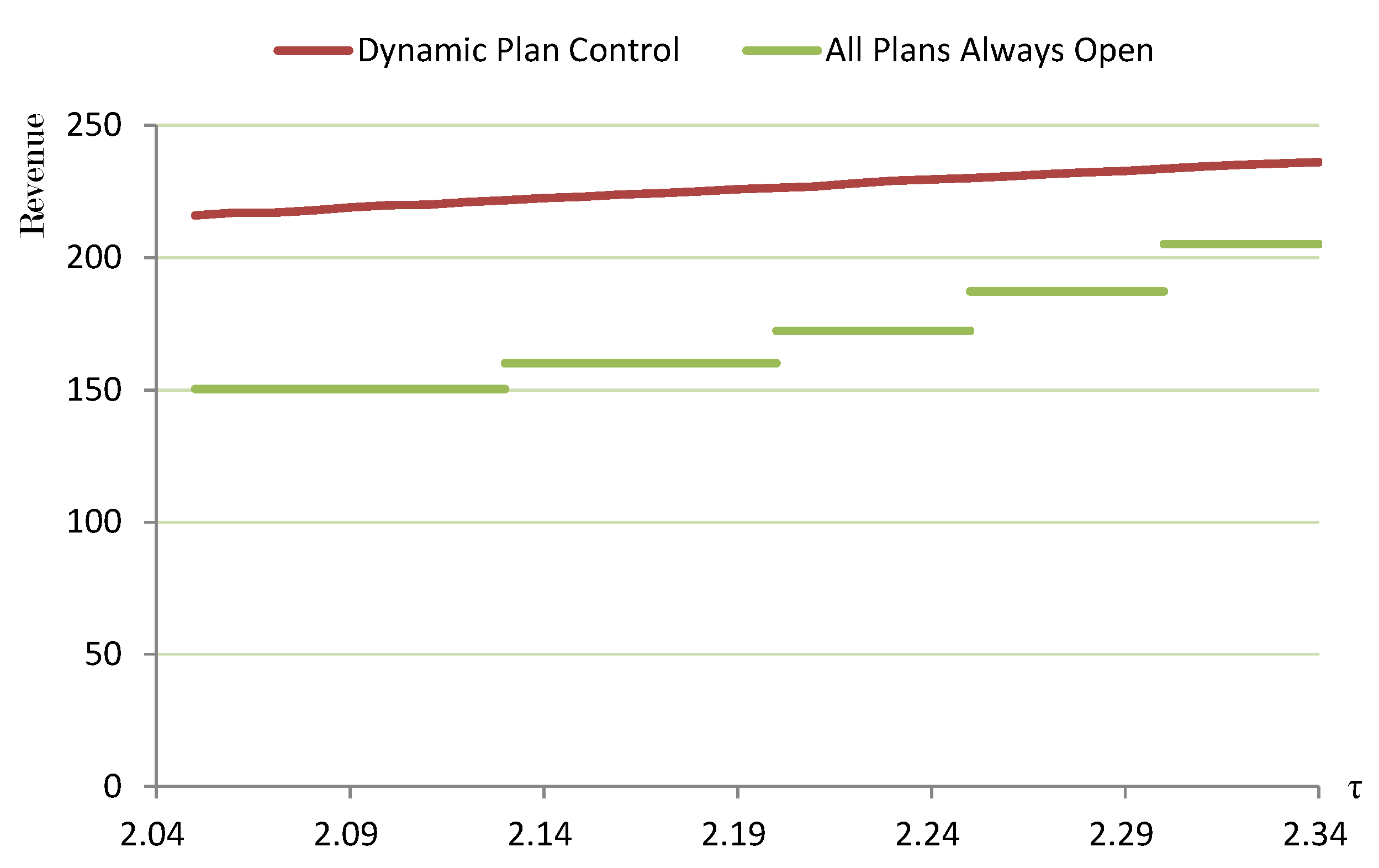
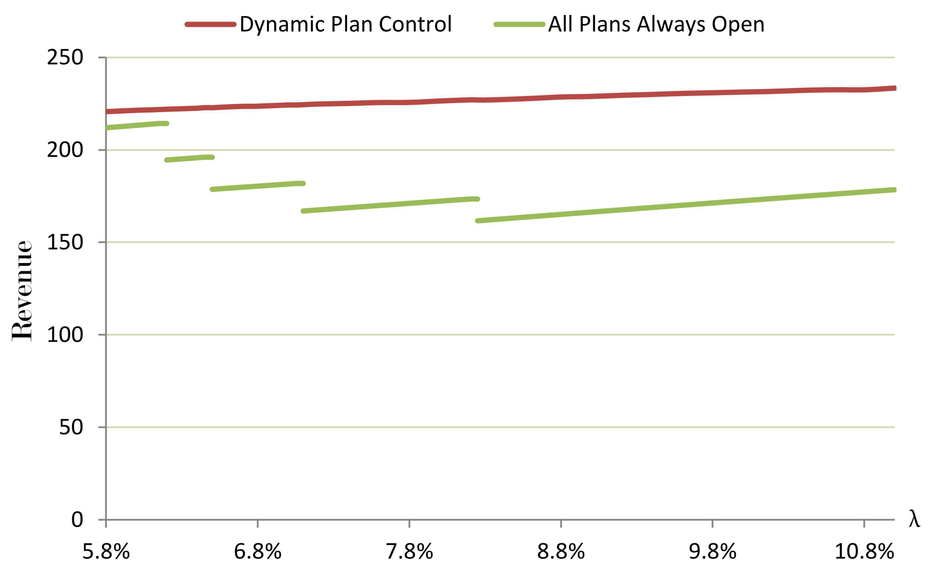
We conclude our findings as follows: (1) After introducing the realistic mechanism of dynamic plan control, we are able to formulate a stochastic dynamic programming problem based on mild and reasonable assumptions about data plan settings and customers’ decision-making procedures. (2) According to Theorem 1 and 2, the dynamic programming problem can be transformed to an equivalent mixed integer linear programming problem, so that the dimension is significantly reduced for efficient computation. (3) The result of numerical evaluation shows that the dynamic plan control method helps a large European mobile service provider manage demand considering congestion and increase its revenue by 31.44%. (4) Compared with the “all plans always open” policy, the proposed dynamic plan control method is able to provide more robust revenue for the service provider when network capacity or the potential customers’ willingness to join the network changes. If a mobile service provider has a small network capacity or its potential customers have a high level of willingness, then it can benefit more from the dynamic plan control method.

Although we summarized three important contributions of this study in Section 1, we suggest the following directions for future research based on current limitations. First, this paper only assumes the connection-speed-restriction pricing scheme, so it would be interesting to implement the dynamic plan control under other types of pricing schemes. Second, our model considers only one mobile service provider. Based on our research, a model with competing mobile service providers would be an interesting extension, especially if these service providers employ different pricing schemes. Finally, since our approach succeeds in the context of wireless telecommunication management, we consider exploring its applications in other similar systems.

References

1. Cisco. Cisco Visual Networking Index: Global Mobile Data Traffic Forecast Update, 2017–2022 White Paper; White Paper; Cisco: San Jose, CA, USA, 2019. [Google Scholar]
2. Hwang, R.H.; Peng, M.C.; Cheng, K.C. QoS-guaranteed radio resource management in LTE-A co-channel networks with dual connectivity. Appl. Sci. 2019, 9, 3018. [Google Scholar] [CrossRef] [Green Version]
3. Ma, X.; Deng, T.; Xue, M.; Shen, Z.J.M.; Lan, B. Optimal dynamic pricing of mobile data plans in wireless communications. Omega 2017, 66, 91–105. [Google Scholar] [CrossRef] [Green Version]
4. Perez-Murueta, P.; Gómez-Espinosa, A.; Cardenas, C.; Gonzalez-Mendoza, M. Deep Learning System for Vehicular Re-Routing and Congestion Avoidance. Appl. Sci. 2019, 9, 2717. [Google Scholar] [CrossRef] [Green Version]
5. Deng, T.; Shen, Z.J.M.; Shanthikumar, J.G. Statistical Learning of Service-Dependent Demand in a Multiperiod Newsvendor Setting. Oper. Res. 2014, 62, 1064–1076. [Google Scholar] [CrossRef]
6. Loiseau, P.; Schwartz, G.; Musacchio, J.; Amin, S. Incentive schemes for Internet congestion management: Raffles versus time-of-day pricing. In Proceedings of the 2011 49th Annual Allerton Conference on Communication, Control, and Computing (Allerton), Monticello, IL, USA, 28–30 September 2011; pp. 103–110. [Google Scholar] [CrossRef] [Green Version]
7. Lee, J.; Yi, Y.; Chong, S.; Jin, Y. Economics of WiFi offloading: Trading delay for cellular capacity. In Proceedings of the 2013 IEEE Conference on Computer Communications Workshops (INFOCOM WKSHPS), Turin, Italy, 14–19 April 2013; pp. 357–362. [Google Scholar] [CrossRef]
8. Cheng, H.K.; Bose, I. Performance models of a proxy cache server: The impact of multimedia traffic. Eur. J. Oper. Res. 2004, 154, 218–229. [Google Scholar] [CrossRef]
9. Cisco. Cisco Visual Networking Index: Global Mobile Data Traffic Forecast Update, 2011–2016; White Paper; Cisco: San Jose, CA, USA, 2012. [Google Scholar]
10. Odlyzko, A. Internet pricing and the history of communications. Comput. Netw. 2001, 36, 493–517. [Google Scholar] [CrossRef] [Green Version]
11. Gizelis, C.A.; Vergados, D.D. A Survey of Pricing Schemes in Wireless Networks. IEEE Commun. Surv. Tutor. 2011, 13, 126–145. [Google Scholar] [CrossRef]
12. Bagh, A.; Bhargava, H.K. How to Price Discriminate When Tariff Size Matters. Mark. Sci. 2012, 32, 111–126. [Google Scholar] [CrossRef]
13. Danaher, P.J. Optimal Pricing of New Subscription Services: Analysis of a Market Experiment. Mark. Sci. 2002, 21, 119–138. [Google Scholar] [CrossRef] [Green Version]
14. Grubb, M.D. Selling to Overconfident Consumers. Am. Econ. Rev. 2009, 99, 1770–1807. [Google Scholar] [CrossRef] [Green Version]
15. Fibich, G.; Klein, R.; Koenigsberg, O.; Muller, E. Optimal Three-Part Tariff Plans. Oper. Res. 2017, 65, 1177–1189. [Google Scholar] [CrossRef]
16. Bhargava, H.K.; Gangwar, M. On the Optimality of Three-Part Tariff Plans: When Does Free Allowance Matter? Oper. Res. 2018, 66, 1517–1532. [Google Scholar] [CrossRef]
17. Sen, S.; Joe-Wong, C.; Ha, S.; Chiang, M. A survey of smart data pricing: Past proposals, current plans, and future trends. ACM Comput. Surv. 2013, 46, 1–37. [Google Scholar] [CrossRef]
18. Sen, S.; Joe-Wong, C.; Ha, S.; Chiang, M. Smart data pricing: Using economics to manage network congestion. Commun. ACM 2015, 58, 86–93. [Google Scholar] [CrossRef]
19. Jiang, L.; Parekh, S.; Walrand, J. Time-Dependent Network Pricing and Bandwidth Trading. In Proceedings of the NOMS Workshops 2008—IEEE Network Operations and Management Symposium Workshops, Salvador da Bahia, Brazil, 7–11 April 2008; pp. 193–200. [Google Scholar] [CrossRef]
20. Joe-Wong, C.; Ha, S.; Chiang, M. Time-Dependent Broadband Pricing: Feasibility and Benefits. In Proceedings of the 2011 31st International Conference on Distributed Computing Systems, Minneapolis, MN, USA, 20–24 June 2011; pp. 288–298. [Google Scholar] [CrossRef]
21. Batur, D.; Ryan, J.K.; Zhao, Z.; Vuran, M.C. Dynamic Pricing of Wireless Internet Based on Usage and Stochastically Changing Capacity. Manuf. Serv. Oper. Manag. 2019. [Google Scholar] [CrossRef] [Green Version]
22. Ha, S.; Sen, S.; Joe-Wong, C.; Im, Y.; Chiang, M. TUBE: Time-dependent pricing for mobile data. Acm Sigcomm Comput. Commun. Rev. 2012, 42, 247–258. [Google Scholar] [CrossRef]
23. Javaid, N.; Ahmed, A.; Iqbal, S.; Ashraf, M. Day ahead real time pricing and critical peak pricing based power scheduling for smart homes with different duty cycles. Energies 2018, 11, 1464. [Google Scholar] [CrossRef] [Green Version]
24. Loiseau, P.; Schwartz, G.; Musacchio, J.; Amin, S.; Sastry, S.S. Incentive Mechanisms for Internet Congestion Management: Fixed-Budget Rebate Versus Time-of-Day Pricing. IEEE/ACM Trans. Netw. 2014, 22, 647–661. [Google Scholar] [CrossRef] [Green Version]
25. Ma, X.; Deng, T.; Lan, B. Demand estimation and assortment planning in wireless communications. J. Syst. Sci. Syst. Eng. 2016, 25, 1–26. [Google Scholar] [CrossRef]
26. Clements, A.E.; Hurn, A.S.; Li, Z. Forecasting day-ahead electricity load using a multiple equation time series approach. Eur. J. Oper. Res. 2016, 251, 522–530. [Google Scholar] [CrossRef] [Green Version]
27. Abbas, N.; Yu, F.; Fan, Y. Intelligent video surveillance platform for wireless multimedia sensor networks. Appl. Sci. 2018, 8, 348. [Google Scholar] [CrossRef] [Green Version]
28. Lee, J.; Yi, Y.; Chong, S.; Jin, Y. Economics of WiFi Offloading: Trading Delay for Cellular Capacity. IEEE Trans. Wirel. Commun. 2014, 13, 1540–1554. [Google Scholar] [CrossRef] [Green Version]
29. Liu, B.; Zhu, Q.; Tan, W.; Zhu, H. Congestion-Optimal WiFi Offloading with User Mobility Management in Smart Communications. Wirel. Commun. Mob. Comput. 2018, 2018, 9297536. [Google Scholar] [CrossRef]
30. Sun, Y.; Xu, L.; Tang, Y.; Zhuang, W. Traffic offloading for online video service in vehicular networks: A cooperative approach. IEEE Trans. Veh. Technol. 2018, 67, 7630–7642. [Google Scholar] [CrossRef]
31. Ning, Z.; Dong, P.; Wang, X.; Obaidat, M.S.; Hu, X.; Guo, L.; Guo, Y.; Huang, J.; Hu, B.; Li, Y. When deep reinforcement learning meets 5G-enabled vehicular networks: A distributed offloading framework for traffic big data. IEEE Trans. Ind. Inform. 2019, 16, 1352–1361. [Google Scholar] [CrossRef]
32. Sen, S.; Joe-Wong, C.; Ha, S.; Chiang, M. Time-Dependent Pricing for Multimedia Data Traffic: Analysis, Systems, and Trials. IEEE J. Sel. Areas Commun. 2019, 37, 1504–1517. [Google Scholar] [CrossRef]
33. Schlereth, C.; Skiera, B.; Schulz, F. Why do consumers prefer static instead of dynamic pricing plans? An empirical study for a better understanding of the low preferences for time-variant pricing plans. Eur. J. Oper. Res. 2018, 269, 1165–1179. [Google Scholar] [CrossRef]
Figure 1. Two part pricing, three part pricing, and connection-speed-restriction pricing.
Applsci 11 00091 g001
Figure 2. Mechanism of connection-speed-restriction pricing.
Applsci 11 00091 g002
Figure 3. Decisions of the potential customers.
Applsci 11 00091 g003
Figure 4. The interval in which plan i is preferred.
Applsci 11 00091 g004
Figure 5. Trends of the market share under APAO and DPC.
Applsci 11 00091 g005
Figure 6. Relationship between revenue and network capacity.
Applsci 11 00091 g006
Figure 7. Relationship between revenue and potential customers’ willingness to join the network.
Applsci 11 00091 g007