Simplified Welch Algorithm for Spectrum Monitoring

Abstract

Power Spectral Density (PSD) is an essential representation of the signal spectrum that depicts the power measurement content versus frequency. PSD is typically used to characterize broadband random signals and has a variety of usages in many fields like physics, engineering, biomedical, etc. This paper proposes a simple and practical method to estimate the PSD based on the Welch algorithm for spectrum monitoring. The proposed method can be easily implemented in most of software-based systems or low-level Field-Programmable Gate Arrays (FPGAs) and yields a smooth overview of the spectrum. The original Welch method utilizes the average of the amplitude squared of the previous Fast Fourier Transform (FFT) samples for better estimation of frequency components and noise reduction. Replacing the simple moving average with a weighted moving average can significantly reduce the complexity of the Welch’s method. In this way, the amount of required Random Access Memory (RAM) is reduced from K (where K is the number of FFT packets in averaging) to one. This new method allows users to adjust the dependency of the PSD on the previous observed FFTs and its smoothness by setting only one feedback parameter without any hardware change. The obtained results show that the algorithm gives a clear spectrum, even in the noisy situation because of the significant Signal to Noise Ratio (SNR) enhancement. The trade-off between spectrum accuracy and time convergence of the modified algorithm is also fully analysed. In addition, a simple solution based on Xilinx Intellectual Property (IP), which converts the proposed method to a practical spectrum analyzer device, is presented. This modified algorithm is validated by comparing it with two standard and reliable spectrum analyzers, Rohde & Schwarz (R&S) and Tektronix RSA600. The modified design can track any signal type as the other spectrum analyzers, and it has better performance in situations where the power of the desired signal is weak or where the signal is mixed with the background noise. It can display the spectrum when the input signal power is 5 dB lower than the visible threshold level of R&S and Tektronix. In both narrowband and wideband scenarios, the new implemented design can still display frequency components 5 dB higher than the noise, while the output spectrum of other analyzers is completely covered by noise.

1. Introduction

The development of intelligent adaptive technology for spectrum monitoring is an emerging topic for signal processing, especially for satellite broadcasting and radio communication signal analysis [1,2,3]. Frequency power distribution and phase represent the system response to changes in bandwidth, gain, phase shift, harmonics, etc. The recent preferred interest of these characteristics is to locate and reduce the interference caused by adjacent signal communication bands or co-channel emissions [4].

A problem exists regarding the accessibility to a clear power spectrum for smaller and more accessible devices. Most of the available devices use complex algorithms and circuitry to present the clearest overview of the spectrum for a specified application [5]. It mostly results in an expensive device that can be difficult to replace and repair or needs heavy algorithms that may be unnecessary for smaller devices and complex to implement. While a reliable spectrum representation is necessary for research and development in the scientific community, some applications do not need the most accurate value if the amplitude ratio and the shape of the spectrum are properly reflected with a simpler method [5].

To obtain the Power Spectral Density (PSD) estimation, there are parametric and non-parametric methods [6]. The non-parametric methods, based on the Discrete Fourier Transform (DFT) [7], do not assume that the data have any structure. Some of the non-parametric methods are the periodogram method [8], which is the squared of the absolute value of the DFT and the Welch’s method [9], which benefits from the average of multiple DFT scans. For the parametric methods, it is assumed that the data follows a certain model [10] and they require a certain amount of past information to calculate the PSD properly. Some examples of parametric methods are the autoregressive model (AR) [11], the moving-average model (MA), the autoregressive moving average (ARMA) [11], etc.

To retrieve this specific data, the most commonly used system is the Fast Fourier Transform (FFT). FFT transforms a window of discrete samples into its frequency domain representation [12]. However, because of the noise, it is not ideal for locating low power interferences and cannot involve several time packets for better estimation of each frequency component. The Welch’s method is based on the Bartlett’s method where as much as 50% of segments can overlap [13]. Finite data causes noise and poor representation in frequency domain. The Welch’s method improves standard periodogram spectrum estimation by averaging over several FFT packets. This involves more time domain samples and surpasses the finite available data limitation.

The purpose of this paper is to introduce a modified version of the Welch’s method and show how it can be embedded in a Field-Programmable Gate Array (FPGA) design with the help of the last available Intellectual Property (IP) cores from the Xilinx Digital Signal Processing (DSP) generator. The structure of the paper is organized as follows: in section two, the DFT [14,15] is briefly explained as well as how the original Welch’s algorithm works. In section three, the modified design of the Welch’s algorithm architecture is explained and the trade-off between time convergence versus PSD estimation is analyzed. The demonstrated simulation results are presented in section four. Section five presents the FPGA design of the proposed method and explains how it is embedded in a Software Defined Radio (SDR) device and improves it to a powerful spectrum analyzer. Moreover, this chapter explains the obtained results from practical tests in comparison with available commercial spectrum analyzers.

2. Fourier Transform and Welch Algorithm

2.1. DFT & FFT

Discrete time signals result from sampling of continuous-time analog signals that are converted into digital values for future analysis. The interval between consecutive measurements is specified by the sampling period. Thus, discrete time signals are not defined between sampling intervals, which means that the highest possible observable frequency cannot exceed the Nyquist limit [16] that is equal to half of the sampling frequency. Even with this known trade-off, the DFT is a powerful tool for analyzing these types of signals since it can reveal the periodicity in the input signal as well as the relative power for each frequency component. The DFT is defined mathematically as:

$$X\left[k\right]= {\displaystyle \sum }_{n=0}^{N-1}x\left[n\right]\times exp\left(\frac{-j2\pi nk}{N}\right) 0 \le k \le N-1$$

(1)

where N is the number of input samples, k is an integer index, $2\pi /N$is the fundamental frequency resolution, $x= \left\{x\left[0\right],x\left[1\right],\dots x\left[n\right]\right\}$is the window of input samples, and $X= \left\{X\left[0\right],X\left[1\right],\dots X\left[n\right]\right\}$ is the vector of DFT samples. The DFT can also be written in a matrix form:

$$\left[\begin{array}{c}X\left[0\right]\\ X\left[1\right]\\ X\left[2\right]\\ ⋮\\ X\left[N-1\right]\end{array}\right]= \left[\begin{array}{ccc}{W}_0^0& \cdots & W_{N-1}^0\\ ⋮& \ddots & ⋮\\ W_0^{N-1}& \cdots & W_{N-1}^{N-1}\end{array}\right]\left[\begin{array}{c}x\left[0\right]\\ x\left[1\right]\\ x\left[2\right]\\ ⋮\\ x\left[N-1\right]\end{array}\right]$$

(2)

where $W=\left[\begin{array}{ccc}{W}_0^0& \cdots & W_{N-1}^0\\ ⋮& \ddots & ⋮\\ W_0^{N-1}& \cdots & W_{N-1}^{N-1}\end{array}\right]$ is DFT coefficient matrix. DFT calculation requires many mathematical operations such as 4N² real multiplications and N (4N − 2) real additions. The FFT is a computational implementation of the DFT and it reduces the complexity of computing the DFT from $O\left(N^2\right)$ to $O\left(Nlo{g}^N\right)$ that is more numerically efficient than the DFT [17].

2.2. Welch’s Method

The main usage of the Fourier transform is to get the frequency samples of an input signal. For a discrete signal, the FFT can be applied to a certain number of samples or, depending on the sampling frequency, a certain amount of time of the signal. Represented spectrum in DFT is limited to half of the sampling frequency. This method is widely used, but the problem is the ambient noise and limitation due to the finite number of samples in the input window. The situation of signals that travel in communication channels is even worse. They experience channel with additive white Gaussian noise (AWGN). Depending on the travelling method and the distance between transmitter and receiver, the noise level may cover the signal and make it harder for the receiver to extract the PSD with acceptable details. In noisy situations, spectrum monitoring requires more and more data time samples for the correct estimation of the frequency components.

The Welch algorithm [18,19] is a nonparametric method to estimate the PSD and it makes the frequency spectrum smoother than the raw FFT output. Let us consider that the FFT is calculated over the entire duration of the signal. In the Welch algorithm, instead of processing the FFT over the entire time domain, the signal is separated in windows with the same size. Window size affects the clarity of the result by cutting frequencies with periods larger than the window. Windowing is taking a sample of a larger dataset and tapering the signal at the edges of each interval. This makes the signal smoother without sharp transitions that can disturb the frequency spectrum representation [11]. There are different types of windowing sequence like Hamming and Blackman, which affect the result differently. Each window overlaps the adjacent windows by a certain factor, which can be as much as 50% of the total window size. Overlapping helps to reduce the loss of information because of the tapering and display a more reliable periodogram. The Fourier transform is calculated on each interval, and the value is squared. This results in a modified periodogram value that is the base of the PSD calculation. Finally, the average of all periodograms are calculated as PSD estimation. Averaging enhances the SNR and it is optimal for spectrum monitoring. The issue with the Welch algorithm is that the frequency resolution is reduced compared to the FFT. Let us consider a discrete time signal $s$ with N samples:

$$s=x\left[1\right], x\left[2\right], \dots , x\left[N\right]$$

(3)

The signal can be separated in K smaller intervals with M length and V overlapping:

$$\begin{gathered} 1:s_1=x\left[1\right], x\left[2\right], \dots , x\left[M\right] \\ 2:s_2=x\left[M-V+1\right], x\left[M-V+2\right], \dots , x\left[2M-V\right] \\ \dots \\ K :s_K=x\left[\left(K-1\right)M-\left(K-1\right)V+1\right], \dots , x\left[KM-\left(K-1\right)V\right] \end{gathered}$$

(4)

where $s_i= \left\{s_i\left[1\right],s_i\left[2\right], \dots s_i\left[M\right]\right\}$ represents the ith window and K is number of the involved window in the PSD calculation. The DFT is calculated for each window:

$$S_i\left[v\right]= {\displaystyle \sum }_{m=1}^M{s}_1\left[m\right]·w\left[m\right]\exp \left(\frac{-2\pi jmv}{N_F}\right) 1\le v\le N_F$$

(5)

where $w= \left\{w\left[1\right],w\left[2\right],\dots w\left[M\right]\right\}$ is the windowing vector, N_F is the DFT size, and$S_i= \left\{S_i\left[1\right],S_i\left[2\right], \dots S_i\left[N_F\right]\right\}$ represent the vector of frequency samples of ith input window. Periodogram values are squared of the absolute value of the DFT samples:

$$P_i\left[v\right]= \frac{1}{C} {\left|S_i\left[v\right]\right|}^2 1\le v\le N_F$$

(6)

where C is normalization factor:

$$C={\displaystyle \sum }_{m=1}^M{w}^2\left[m\right]$$

(7)

Calculated periodogram values from different windows are averaged and the Power Spectral Density estimate is obtained:

$$PSD\left(v\right)= \frac{1}{K}{\displaystyle \sum }_{i=1}^K{P}_i\left[v\right] 1\le v\le N_F$$

(8)

The number of packets involved in averaging directly affects the estimated PSD in different ways. First, as more packets are involved, estimation uses more past data and a smoother spectrum is obtained. In other words, average order K is controlling the dependency on the past. Larger K values help the system to estimate each frequency component based on more observations. Second, if there are fast variations in a frequency component (like a carrier with a hopping center frequency), large averaging can have some drawback on estimation and stop the system from monitoring the fast variations in spectrum. Thus, a robust monitoring system needs to have a variable K to adjust itself from time to time based on the situation. For example, if the target is to detect a weak frequency component under noisy conditions, a K with a larger value can help the monitoring system to recognize it more clearly. In other situations, when the system is trying to track a fast-hopping carrier frequency, smaller K values are more useful because the averaging over time can filter fast variations.

Implementing this moving average requires K number of Random Access Memory (RAM) blocks with N_F size that save observed FFT vectors for averaging. Thus, the complexity and required space on FPGA depends directly on the considered number of FFT packets for averaging. Another drawback is that to support a device with variable average order K, one has to provide K_max RAMs in FPGA and use as much as is required depending on the situation.

3. Modified Welch Algorithm

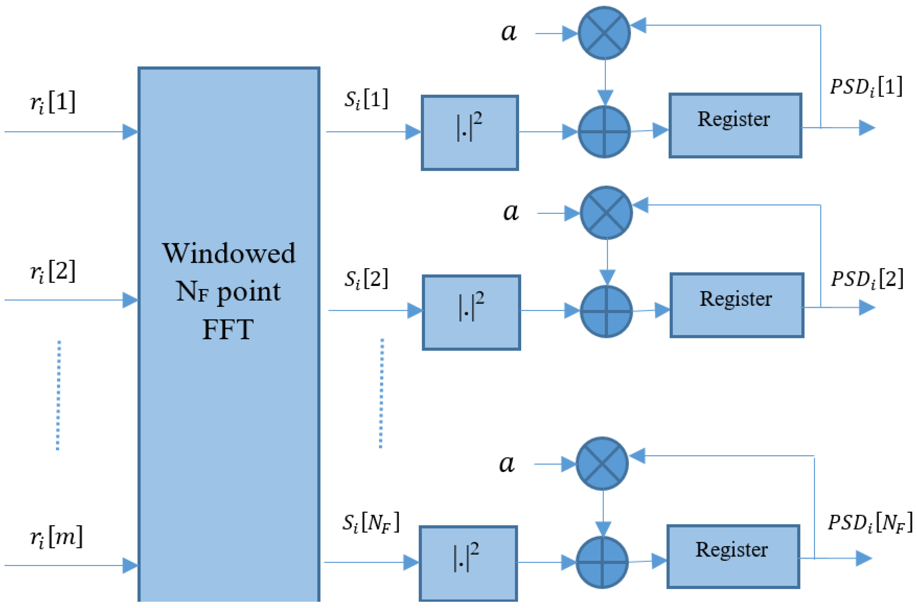
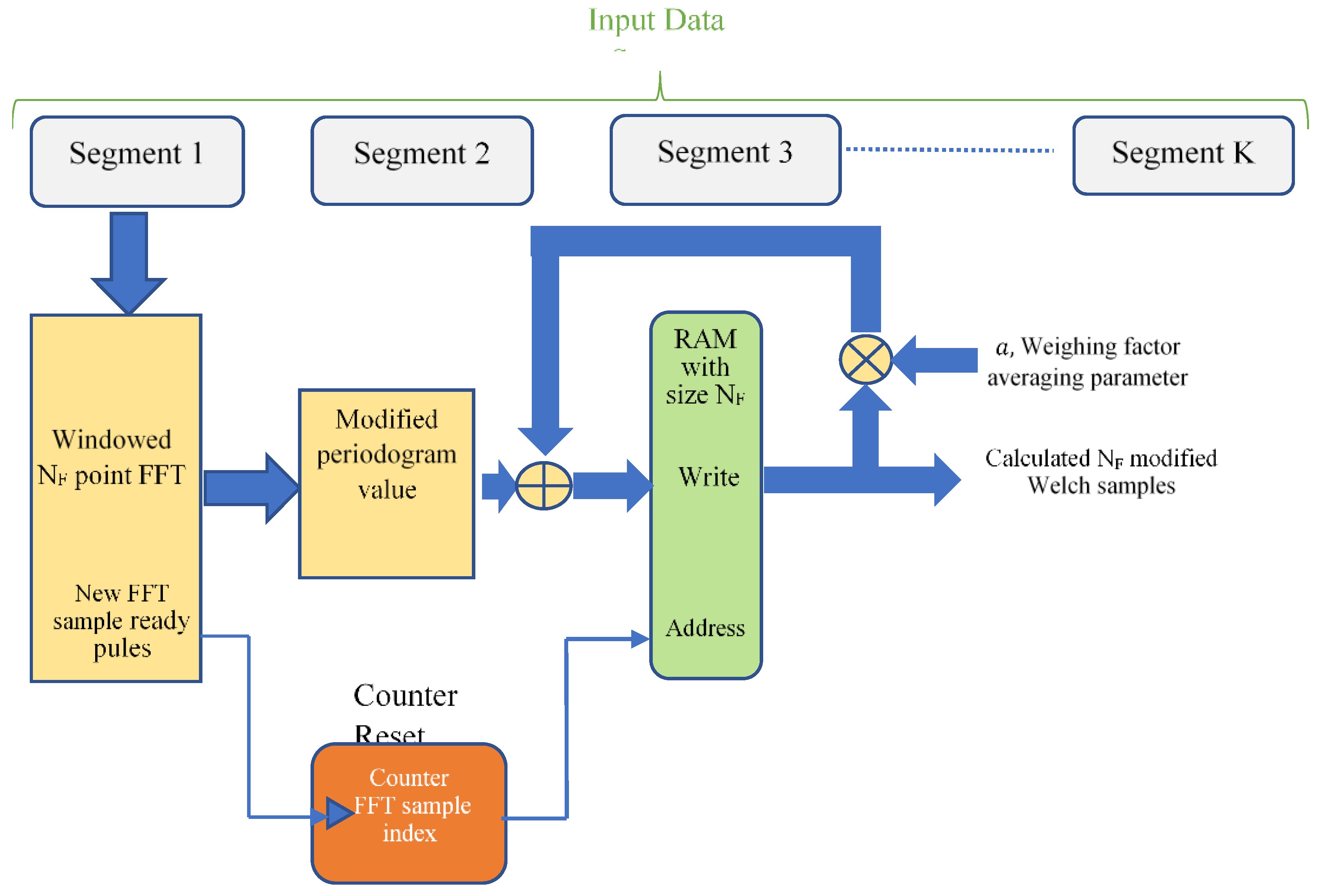
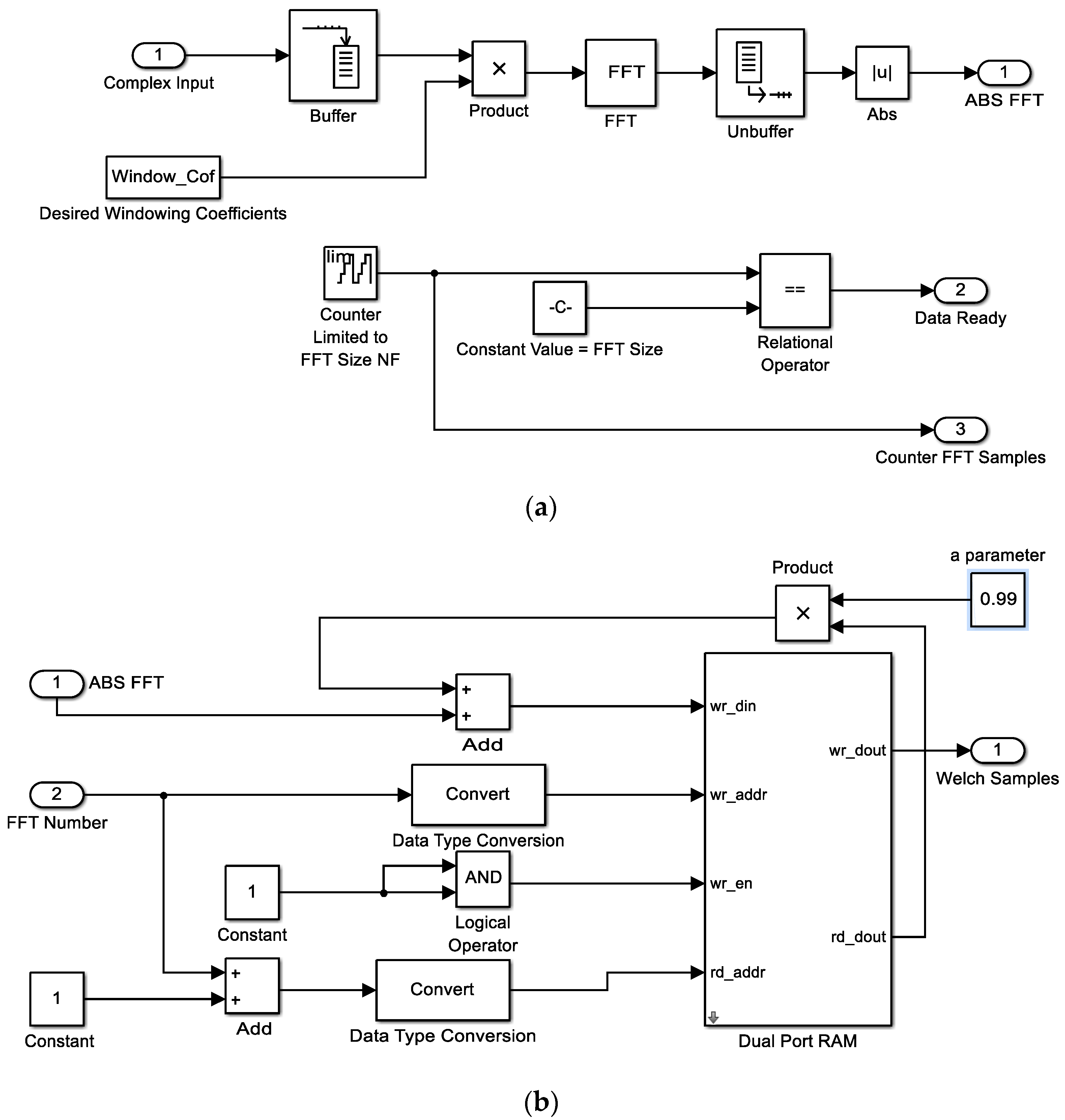
3.1. Proposed Algorithm

As presented before, the Welch samples are an estimation of the power spectral density based on the arithmetic average of multiple FFT [20] scans. The modified version replaces the running average by weighted averaging to simplify and allow for real-time calculation. To better explain this concept, let us consider the moving average over an input data stream by a window with the size of N_p. The result can be expressed by the following Equation (9):

$$y_i=\frac{1}{N_p}{\displaystyle \sum }_{m=0}^{N_p-1}{x}_{i-m}$$

(9)

where y_i is the moving average at sample time i and x_i is the input data stream. The Welch algorithm uses averaging (or arithmetic averaging) in order to achieve two important goals:

• SNR improvement: averaging over more samples can reduce the noise power level and enhance the SNR of desired signal.
• Precise estimation: by utilizing FFT samples from the past, each frequency component can be estimated with more precision.

However, arithmetic averages of past samples have the following consequences [21]:

• Implementing arithmetic averaging of N order, requires N RAM components and massively increases the complexity for real time implementation.
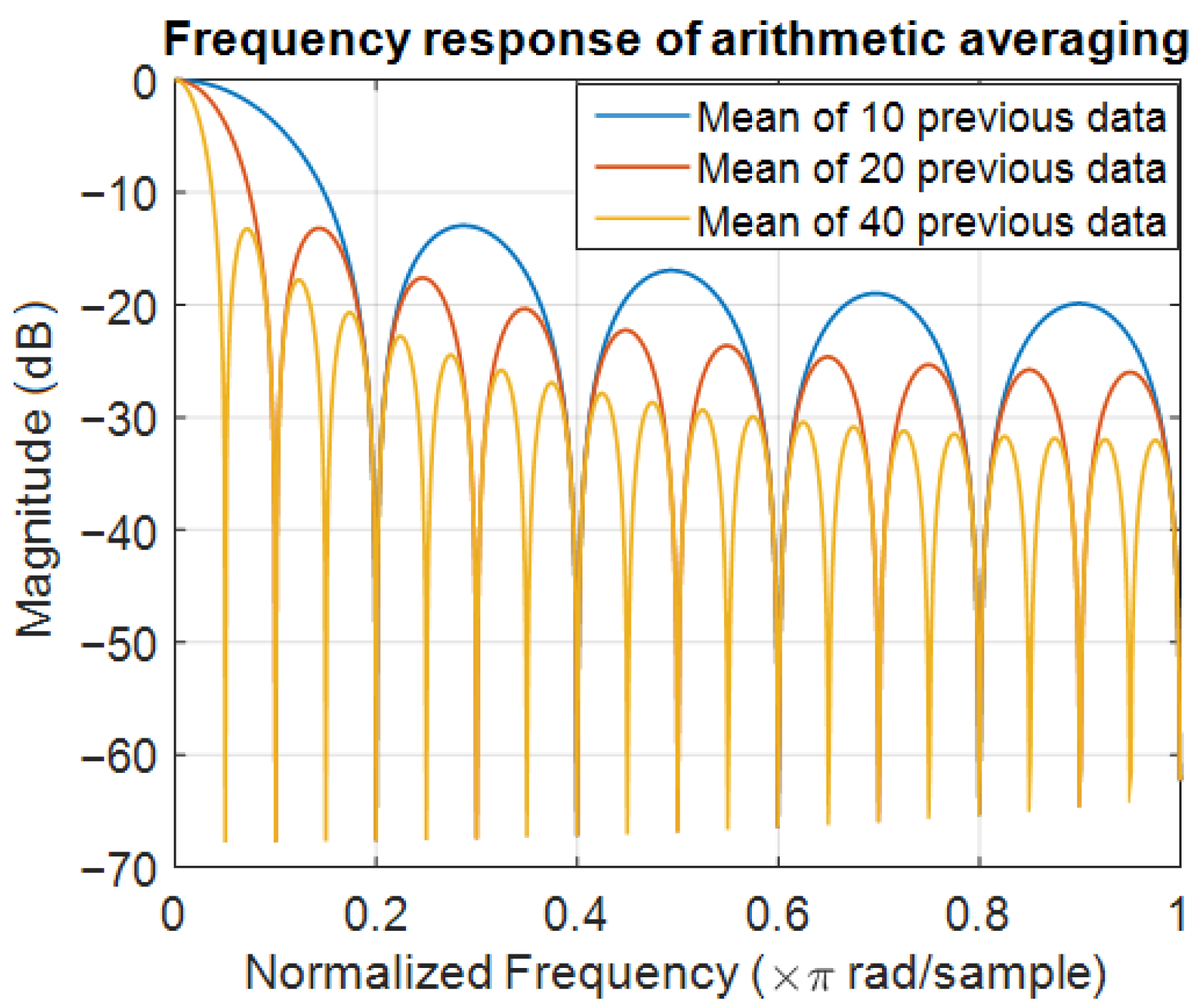
• All the previous samples are weighted by the same coefficient. For example, the sample with distance of 10 time intervals from the current sample is weighted by the same gain as the sample with the distance of 100 time intervals. However, in many systems, it is suitable to weight the samples based on their distance from current samples.

Weighted averaging is widely used in the digital signal processing domain, especially in image processing for noise reduction and signal enhancement [22,23]. In the image processing area, weighted averaging helps greatly with the noise reduction while preserving the fast variations in image edge. In such filtering scenarios, pixels in filtering windows are weighted based on their distance from the central pixel.

This paper tries to replace the arithmetic averaging by the weighted averaging to target two important points:

• Weighting each FFT packet based on its distance from the current packet, this idea helps to preserve the fast variable frequency component in spectrum.
• A recursive and simple algorithm can replace the required memories for the arithmetic averaging.

It means that the system should weight samples based on their distance from the current time instance:

$$y_i^{\prime }=\frac{1}{G}{\displaystyle \sum }_{m=0}^{N_p-1}{\alpha }_m{x}_{i-m} , {\alpha }_0>{\alpha }_1>{\alpha }_2\dots >{\alpha }_{N_p-1}$$

(10)

where $G= {\displaystyle \sum }_{m=0}^{N_p-1}{a}_m$ is normalization gain, $y_i^{\prime }$ is calculated weighted average in ith interval, and $\left\{{\alpha }_0,{\alpha }_1,{\alpha }_2\dots {\alpha }_{N_p-1}\right\}$ are utilized weighting coefficients. The dependency degree for each input sample is determined by selected weighting coefficient ${\alpha }_m$. Now, the dependency of $y_i^{\prime }$ is extended to the past by replacing all the independent weights by exponential weights.

$$y_i^{\prime }=\frac{1}{G}{\displaystyle \sum }_{m=0}^{N_p-1}{\alpha }^m{x}_{i-m} , 0<\alpha <1 and G= {\displaystyle \sum }_{m=0}^{N_p-1}{a}^m$$

(11)

To make the averaging simple and recursive, we first extend the dependency to all previous input samples:

$$y_i^{\prime \prime }= \frac{1}{G}{\displaystyle \sum }_{m=0}^{\infty }{\alpha }^m{x}_{i-m}$$

(12)

$\mathrm{where} G= {\displaystyle \sum }_{m=0}^{\infty }{\alpha }^m$ and $x_i=0$for $i<0$ and $y_i^{\prime \prime }$ is the weighted averaging of all the past input samples. Now, a recursive algorithm can be extracted:

$$\begin{gathered} y_0^{\prime \prime }= x_0 \\ {y}_1^{\prime \prime }= x_1+\alpha x_0= x_1+ a{y}_0^{\prime \prime } \\ {y}_2^{\prime \prime }= x_2+\alpha x_1+{\alpha }^2{x}_0 = x_2+ a{y}_1^{\prime \prime } \\ {y}_3^{\prime \prime }= x_3+\alpha x_2+{\alpha }^2{x}_1+{\alpha }^3{x}_0 = x_3+ a{y}_2^{\prime \prime } \\ \Rightarrow y_i^{\prime \prime }=a\times y_{i-1}^{\prime \prime }+x_i , 0<\alpha <1 \end{gathered}$$

(13)

Equation $PS{D}_i\left[v\right]=a\times PS{D}_{i-1}\left[v\right]+P_i\left[v\right]$ allows us to calculate an averaging with a single multiplication and addition. Figure 1 explains how this principle is applied to all FFT samples.

The displayed design in Figure 1 explains the basic idea, but its implementation is still complex because of several reasons:

• This design needs each FFT sample to implement weighted averages separately, thus the amount of multiplications and summations will increase significantly.
• It is not flexible enough to support different FFT sizes. For example, if the FFT size changes from 1 K to 2 K, all of the design must change completely to support it.
• Certain types of FFT blocks, e.g., in the Xilinx DSP Generator library, work in a series manner that makes the design more complex.

Given these reasons, a simple solution with the help of the RAM is presented to calculate Welch samples based on the weighted averaging. Figure 2 symbolically explains the modified design of Welch implementation. This design reduces the required memory to single RAM by NFFT address. Each averaged FFT samples are added to the previous averaged samples that are multiplied by the $\alpha$ factor. The only consideration here is the use of a FFT computation in series instead of a parallel version.

For each segment of input data stream with the length of M, a windowed $N_F$ point FFT is calculated. After the M clock, M samples of a segment enter this block, then it calculates the $N_F$ point FFT of this sample. After calculation, FFT samples are ready at the output, sample by sample and synchronized with the clock. Each time that FFT samples of an input segment are ready, the FFT block generates a “Data Ready” pulse that determines the start point of the sample series. The “Data Ready” pulse is used to reset a counter. The output number of the counter will read the previous value and save the FFT sample into the RAM at the correct address where each address is a specific frequency PSD estimation.

3.2. Theoretical Analysis

The following analysis explains the equivalency between weighted averaging with the α parameter and arithmetic averaging with N order based on the Signal to Noise Ratio (SNR) enhancement. SNR is defined as:

$$SNR=\frac{P_S}{P_Z}$$

(14)

where $P_S$and $P_Z$are the input signal and the white Gaussian noise power respectively. Reference [24] explains the effect of signal averaging on a steady signal S with an associated noise variance of ${\sigma }^2$. It is proven that if observed signals in averaging iteration are correlated, after N time averaging, $SN{R}_{Averaging}$ is improved by factor of N:

$$\begin{gathered} SN{R}_{Averaging}=N·SNR \\ SN{R}_{Averaging}\left[\mathrm{dB}\right]=10lo{g}_{10}^N+SNR\left[\mathrm{dB}\right] \end{gathered}$$

(15)

Following the same way as [24], it can be proven that for weighted averaging $SN{R}_{Averaging}^{weighted}$ is improved by factor $\frac{1}{1-a}$:

$$\begin{gathered} SN{R}_{Averaging}^{Weighted}=\frac{1}{1-a}·SNR \\ SN{R}_{Averaging}^{Weighted}\left[\mathrm{dB}\right]=10lo{g}_{10}^{\left(\frac{1}{1-a}\right)}+SNR\left[\mathrm{dB}\right] \end{gathered}$$

(16)

For better understanding, the same scenario has been simulated. First, a discrete signal with 1000 samples is generated and white Gaussian noise with SNR = 15 dB is added to the desired signal. Then, the system tries to increase the SNR with the help of two different averaging types. Figure 3c displays $SN{R}_{Averaging}$ versus order N. Clearly, more $SN{R}_{Averaging}$ improvement is obtained by increasing the N order. In another figure, the output $SN{R}_{Averaging}^{Weighted}$ after weighted averaging with different α parameter is displayed. It can be seen weighted averaging with α = 0.99 improve SNR by the gain around 20 dB. These two figures allow the user to see which α parameter in weighted averaging is equivalent to which N order in normal averaging. Based on this comparison, α = 0.99 is equivalent to normal averaging with order N = 100. This comparison allows the user to select the α parameter based on two new criteria:

• Desired SNR improvement for system
• Equivalent average ordering N in normal Welch algorithm

The parameters selected for the weighted averaging directly affects the behavior of the system in two ways:

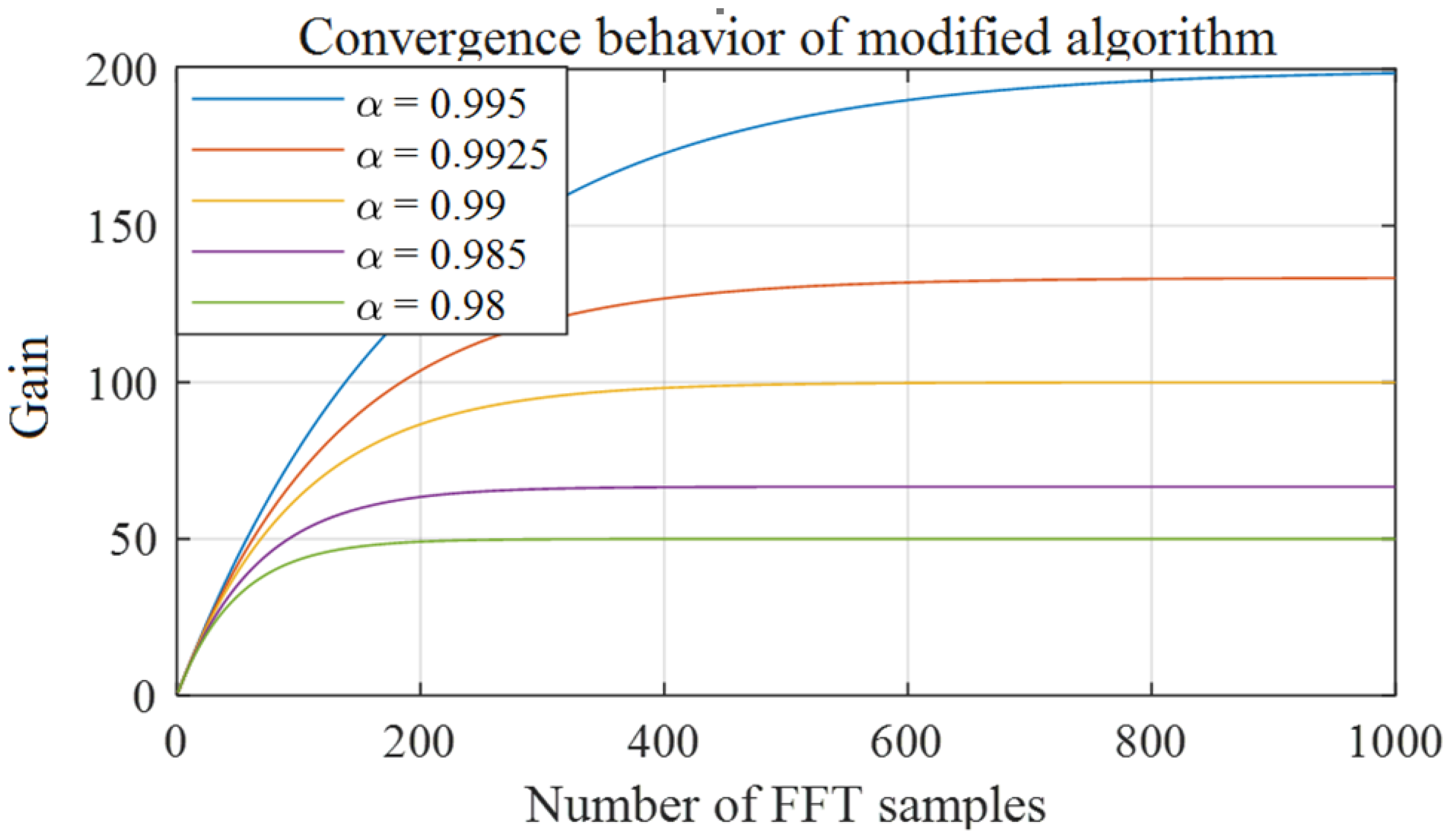
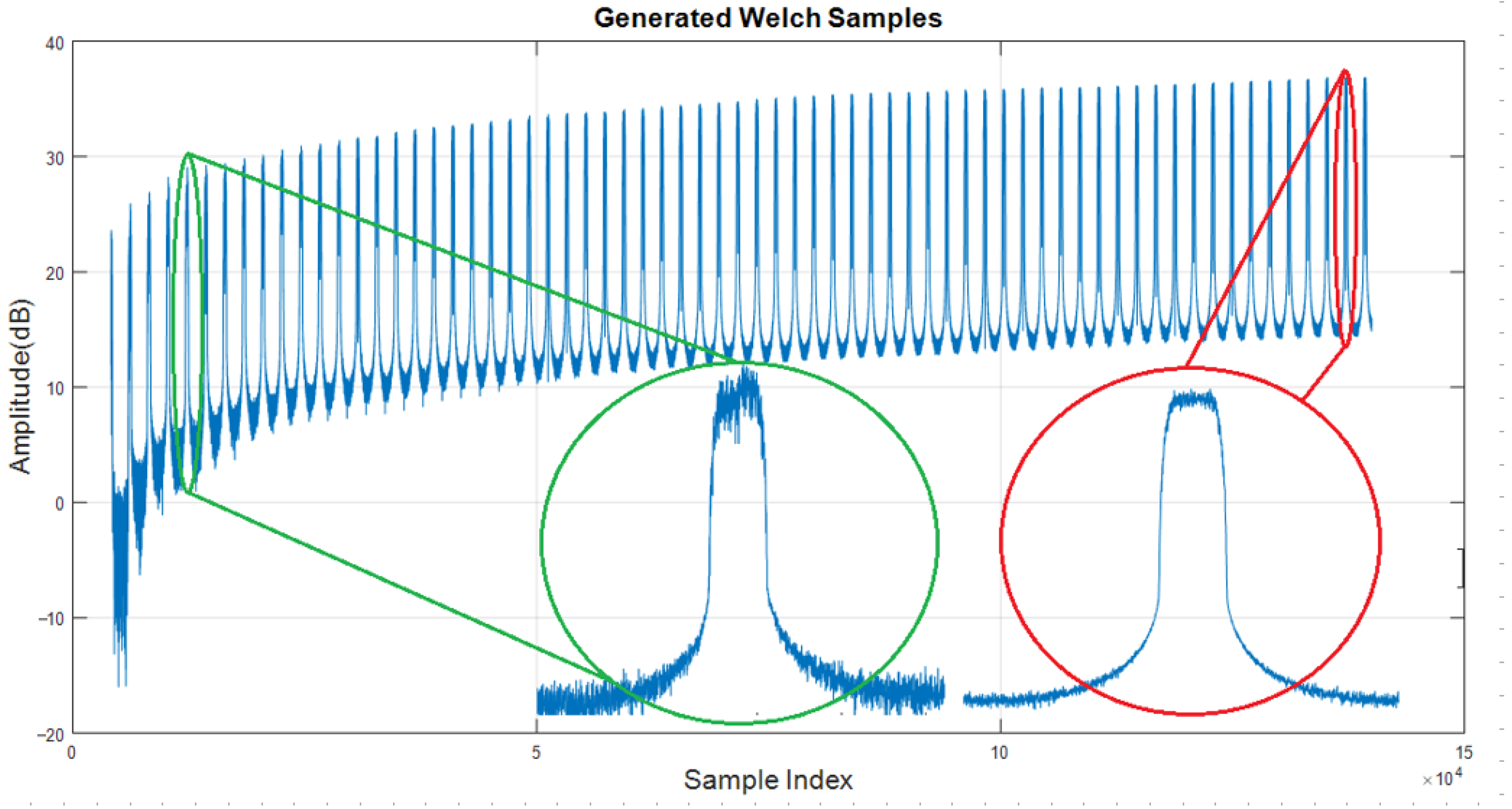
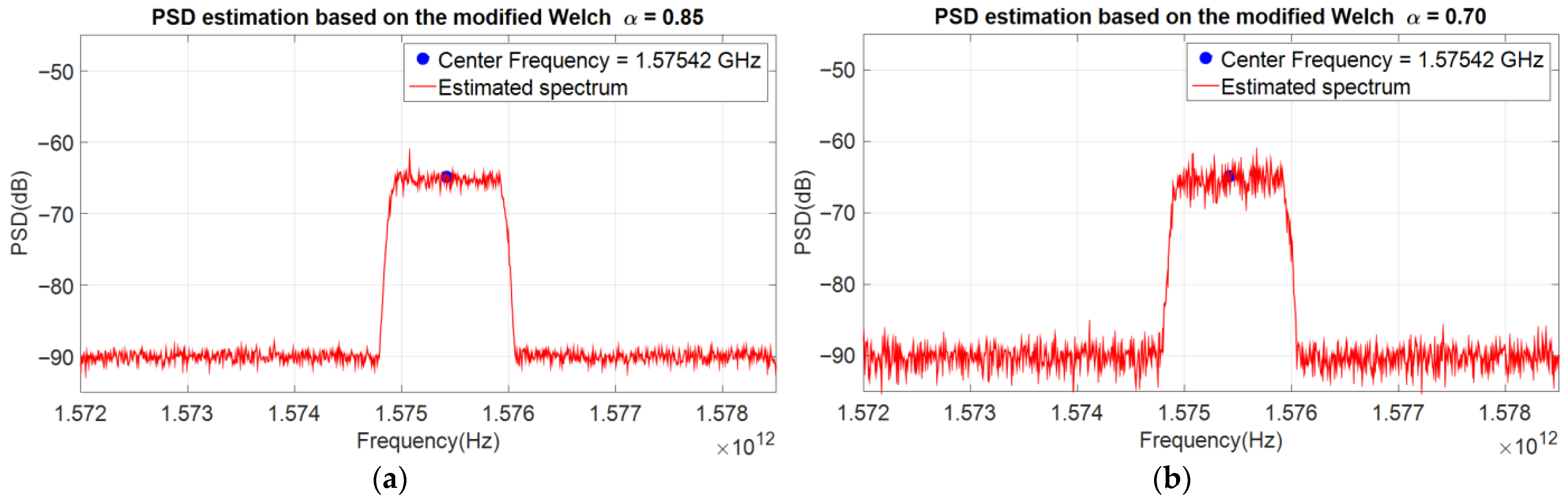
• Convergence time: At first, it seems that the sorted values inside the RAM will grow to an unlimited value. However, because α is smaller than one, the sorted values (Welch spectrum) grow to a certain value and after that the system will converge to a final spectrum. A larger α needs more convergence time and generates larger sorted values in the RAM. Thus, if the system is monitoring data with fast variations, smaller values should be used to enable faster tracking. Another important point here is the hardware limitation for saving the large values inside the RAM. If the saved values are larger than the computational capability of system, a saturation error will happen.
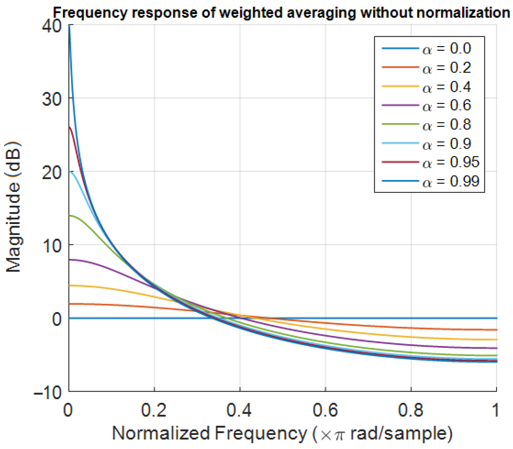
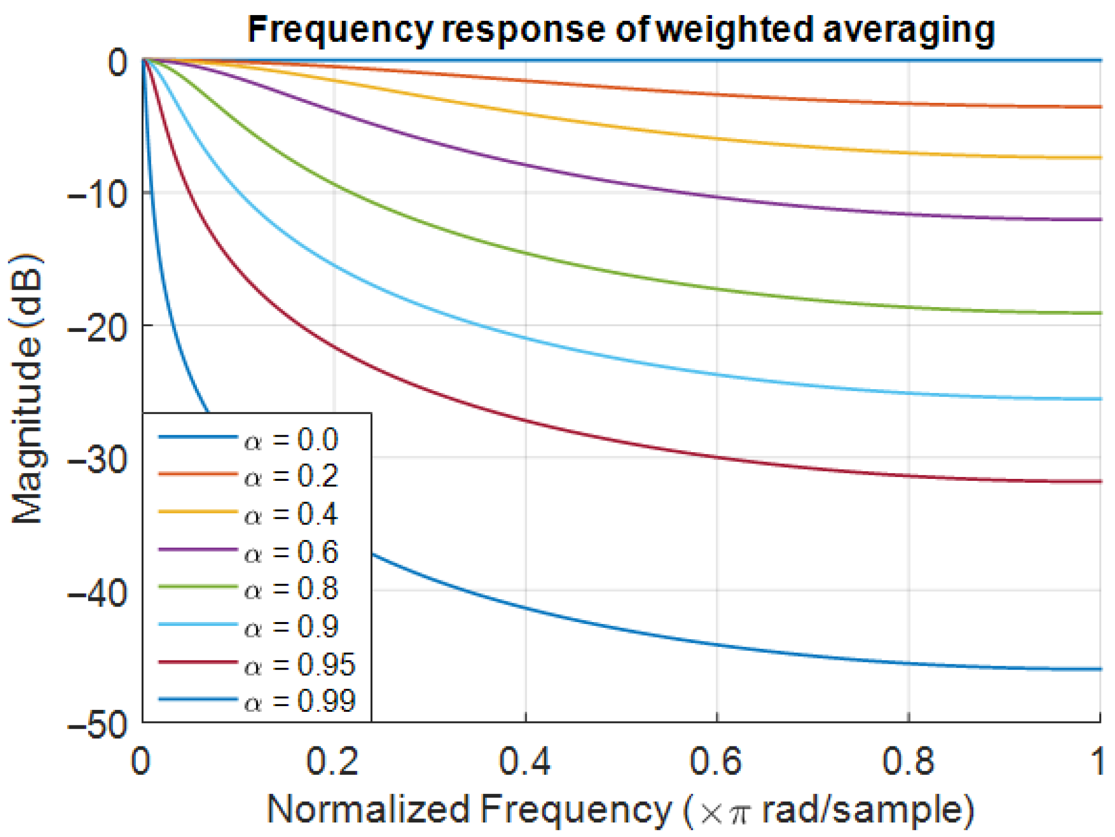
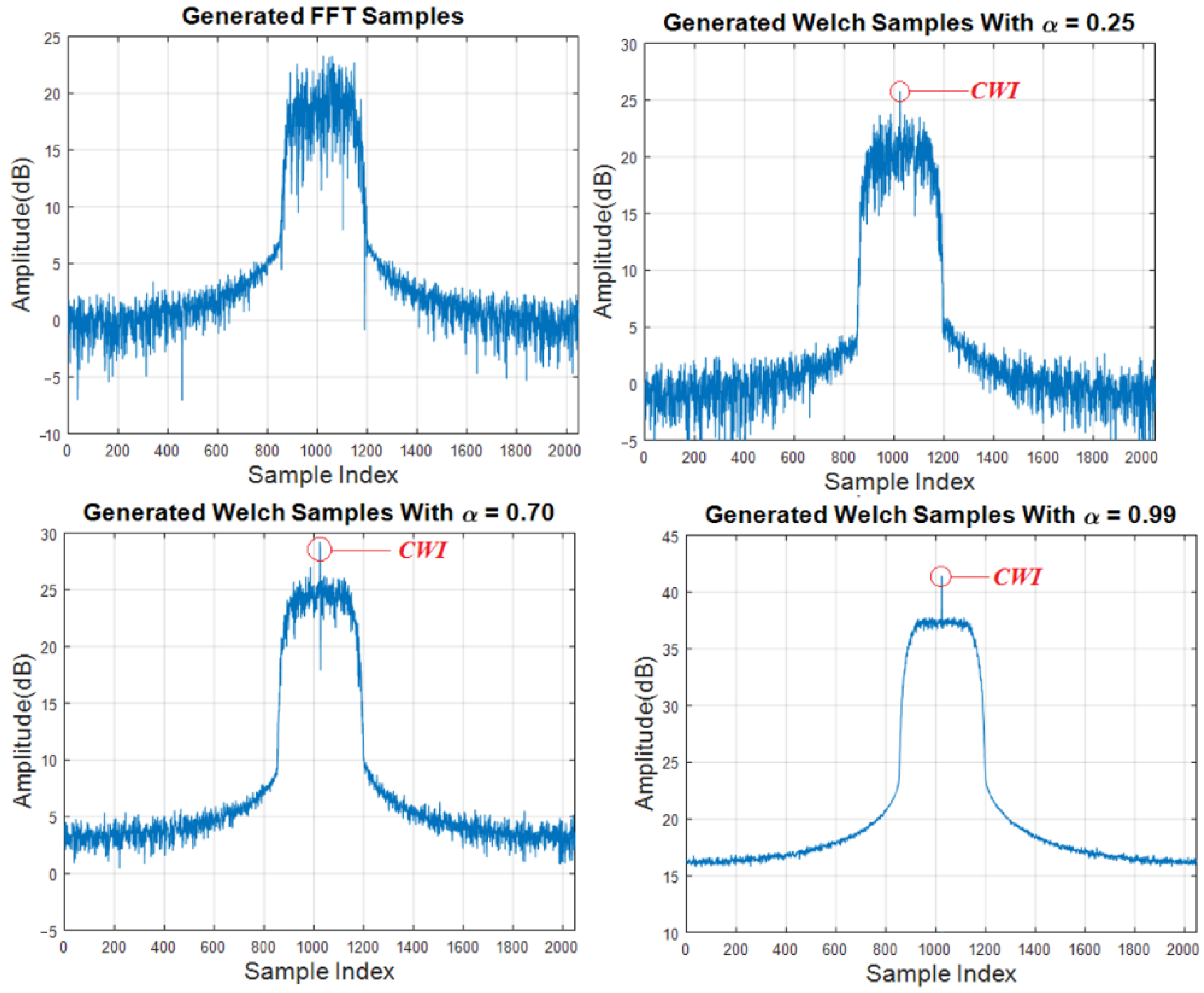
• Obtained spectrum shape: The α determines the dependency of the obtained spectrum to the past. A larger α means more averaging over the past FFT samples. As a result, the spectrum obtained from a larger α is smoother with the less noise.

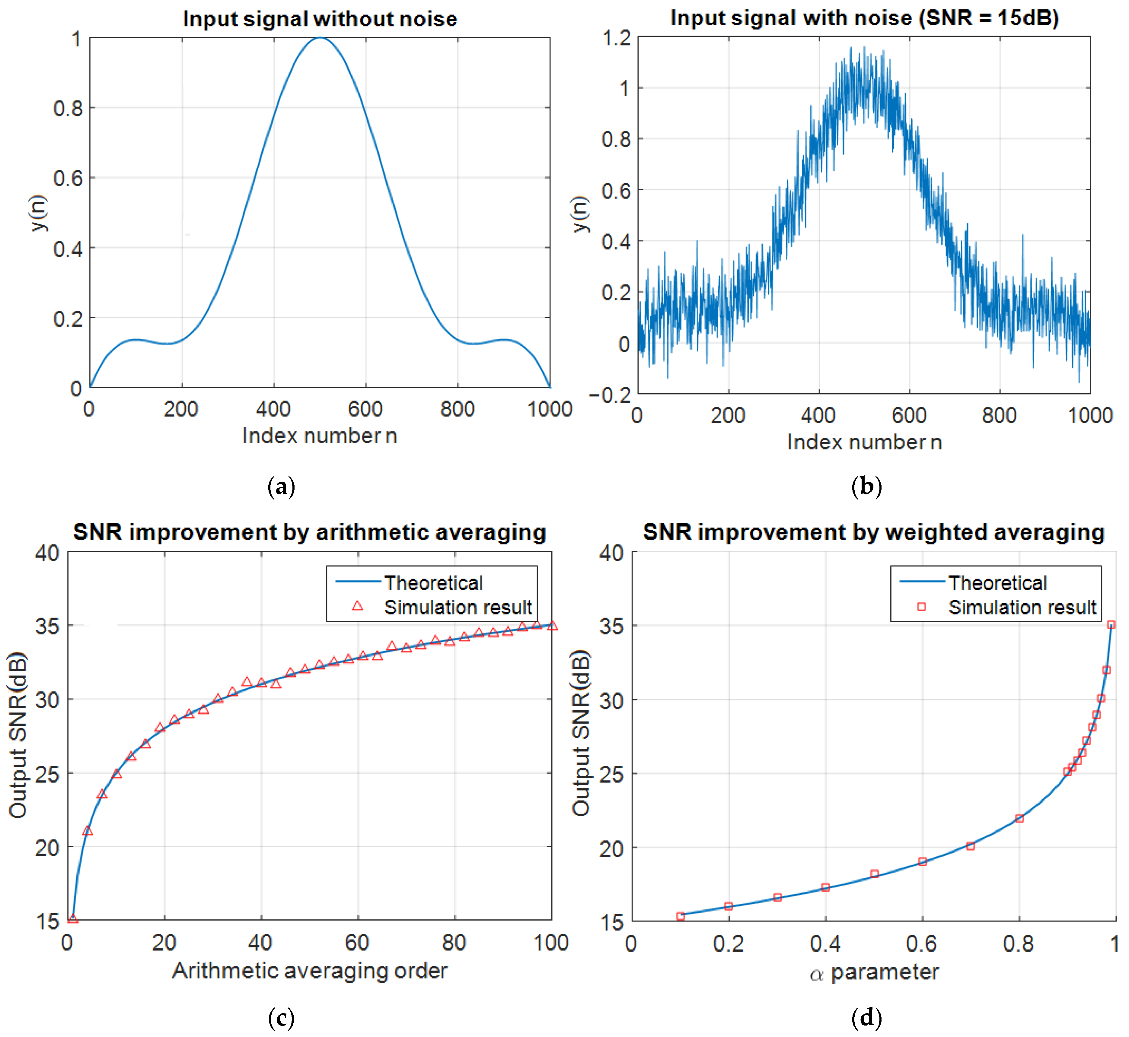
To better understand the difference between the original Welch method [7] and this modified method, the frequency response of a running average is compared to the weighted averaging. Running average has the following frequency response:

$$H\left(z\right)=\frac{1}{N}{\displaystyle \sum }_{i=0}^N{z}^{-i}$$

(17)

Figure 4 presents frequency response of the arithmetic average with different order N. The frequency response is generally attenuated and for averaging with larger order, larger attenuation is observed.

The transfer function of the modified version can be expressed as the following:

$$H\left(z\right)=\frac{1}{1-\alpha z^{-1}}$$

(18)

Figure 5 represents the frequency response of the modified method. Since it is a first order discrete low-pass filter, the curve is significantly smoother for each frequency. As seen below, a higher α value creates a greater initial gain.

As it can be seen in Figure 6, the convergence time and gain are different for each different alpha (α) (feedback factor) value. By analyzing the system response, a normalization factor can be added after the modified Welch algorithm to cancel the gain based on the α parameter.

Final gain G for the selected parameter can be calculated based on the infinite geometric series:

$$Gain G= {\displaystyle \sum }_{m=0}^{\infty }{a}^m=\frac{1}{1-a}$$

(19)

Then the normalization factor (NF) is:

$$NF=1-\alpha$$

(20)

The correction can be added after the algorithm to retrieve a normalized PSD. Figure 7 presents the corrected transfer function of the modified Welch algorithm after the normalization. Comparing Figure 4 with Figure 7 reveals that both systems attenuate frequency components with fast variation, but the modified version has a smoother and more uniform response than the original one and removes the big gaps in frequency response of moving average.

The final point to address is the saturation time based on the α factor. Since the formula is exponential, the following expression can be used to estimate the number of FFT scans until a certain precision of the saturation for a noiseless signal:

$$Number of scans=\frac{{log}_{10}\epsilon }{{log}_{10}\alpha }$$

(21)

where ε is the precision of the saturation. The number of scans is an approximation of the total required FFT packets until partial saturation.

4. Simulations

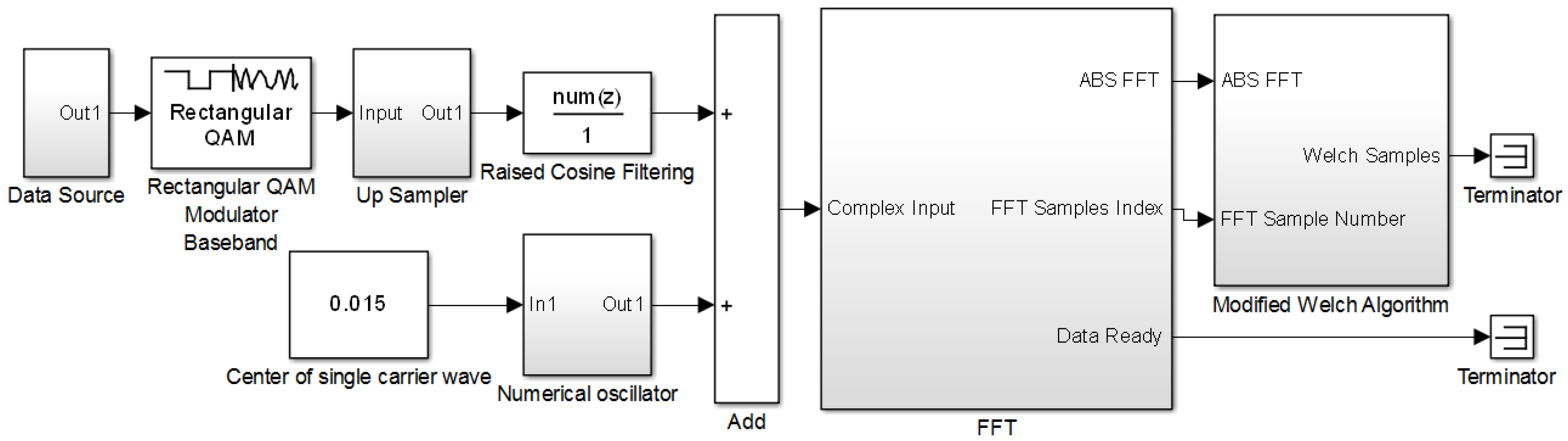
4.1. Simulation Setup

This section explains how the modified algorithm can be implemented simply in MATLAB Simulink as a development environment. Figure 8 displays the block diagram of the design in Simulink. First, the signals are generated on the left, then they are combined and passed through the FFT block mentioned earlier to finally be processed by the updated Welch algorithm. A random data source generates a proper integer numbers for the Quadrature Amplitude Modulation (QAM) modulator. Then, a general telecommunication signal is generated by up sampling and pulse shaping based on raised-cosine filtering. The numerical oscillator generates a single tone at the desired center frequency. The idea here is to show how dependency on past data ($a$ parameter) can obtain a smoother spectrum and help to clarify the Carrier Wave Interference (CWI) [25] as a frequency component. Numerical control oscillator generates CWI based on the selected center frequency $f_0$:

$$CWI=exp\left(j·f_0·t\right)$$

(22)

For example, in Figure 8, a single tone with a peak at the center frequency $f_0=0.015\left(\times \pi \frac{radian}{samp}\right)$ is generated.

The schematic of the implanted FFT and modified algorithm can be seen in Figure 9a,b. The simulation design tries to have the similar behavior of the Xilinx DSP Generator blocks. Samples are first stored into a buffer of FFT size (N_F). After buffering N_F samples, the FFT block transfers the samples to the frequency domain and generates the FFT vector. The FFT vector is then converted to a series of data with the help of the un-buffer block. A free running counter generates the index of FFT samples. Because this counter is limited to count to N_F, after reaching N_F, it will reset to one and start to count up again. In this way, for each packet of FFT samples, the counter generates the correspondence index from one to N_F. The relational block simply compares the counter output with N_F and generates a pulse if the output is equal to N_F as the data ready pulse. This pulse determines the boundaries of each calculated packet in the data stream. It should be mentioned that in the Xilinx DSP Generator, all sub-blocks of the buffer, FFT calculator, un-buffer, counter and data-ready are integrated as one component. The general implementation idea is explained in Figure 9b, where the output of the RAM is multiplied with $a$ in feedback and then added to the new FFT samples to generate the exponential weighted averaging.

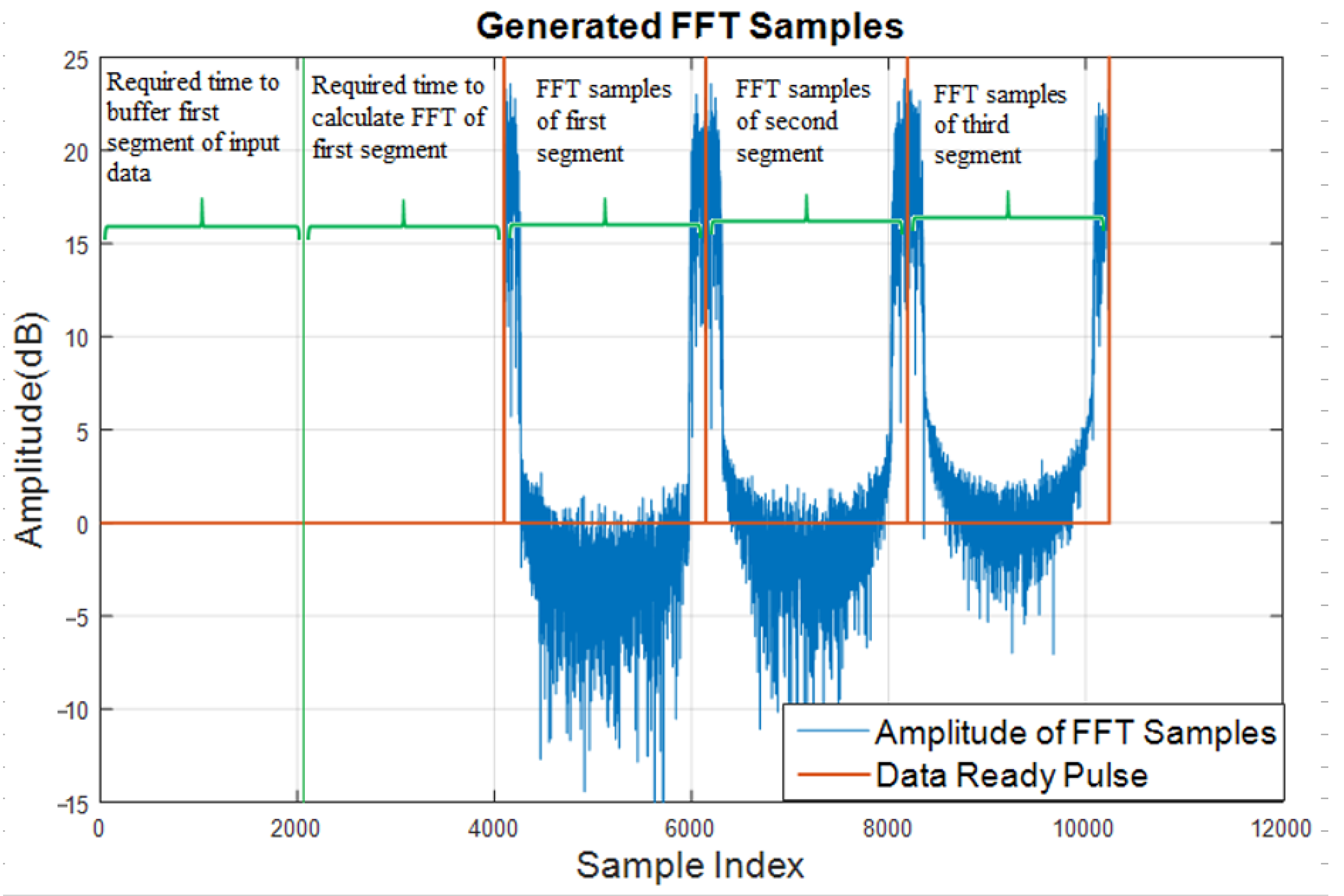
4.2. Simulation Results

As it can be seen in Figure 10, FFT samples are generated by $2\times N_F$ delays. In first $N_F$ clocks, the $N_F$ input data of the first segment is arriving and buffered for FFT calculation. In the second $N_F$ clocks, the FFT of the first input is calculated. While the FFT of the first segment is calculating, the input data of the second segment is buffering. This sequence continues and calculates the FFT of input segments in real time by 2 × $N_F$ delays for all segments.

Another important note here is that the generated FFT samples are displayed from 0 to 2π instead of −π to π. To solve this problem, the first half of the FFT samples must be shifted after the second half to recover the standard spectrum centered at the desired frequency.

After the periodogram values are calculated, they are saved inside the RAM. Each sample is saved in a memory address based on its number in the FFT vector. For example, the 100th periodogram sample is stored in the register with an address equal to 100 in RAM. The idea for calculating a Welch sample is to perform weighted averaging before saving data in each RAM register. Remember that the counter resets with the “Data Ready” pulse, thus, at each moment, the counter value is displaying the corresponding FFT sample number. The output value of the counter is also used to determine the address of this sample inside the RAM. Before overwriting new samples on its related address, the design fetches the previous sample, weighs it with the $\alpha$ parameter and then adds it to the new generated sample. This idea calculates the Welch value based on the weighted averaging. As time goes on, the samples saved inside the RAM converge to Welch samples.

Figure 11 displays the convergence of Welch samples to the final spectrum for α = 0.99 from the simulation. As it can be seen, two spectra generated during the convergence time are displayed. The first spectrum generated is noisier and displays a spectrum of input data with fewer details. After convergence, the spectrum is completely smooth with considerably less noise.

To better understand the performance obtained over the FFT and the effect of the α parameter on the final spectrum, Figure 12 displays the computed spectrum with a different α. During this test, a CWI with Signal to Interference Ratio SI = R12 dB is added to the transmitted signal. For FFT samples, the peak position of CWI fades in the noise and other frequency components make it barely visible. For the Welch spectrum obtained with α = 0.25, the peak is detectable; however, the distance between the maximum peak and the other frequency components is not sufficiently visible and can be misleading for a detector. As the α parameter increases, the spectrum gets smoother and clearer. For α = 0.99, the spectrum is completely smooth, without most of the noise, and the peak appears clearly with a noticeable distance on top of the original signal.

As is explained here, in the modified version, the $\alpha$ parameter plays the same role of the averaging number in the original Welch algorithm. The main advantage of using the modified version is the simplicity and flexibility of the averaging control. The $\alpha$ parameter is like a flexible control volume in the user’s hand and allows the PSD parameters to be adjusted based on the current situation.

5. Laboratory Tests and Real-Time Validation

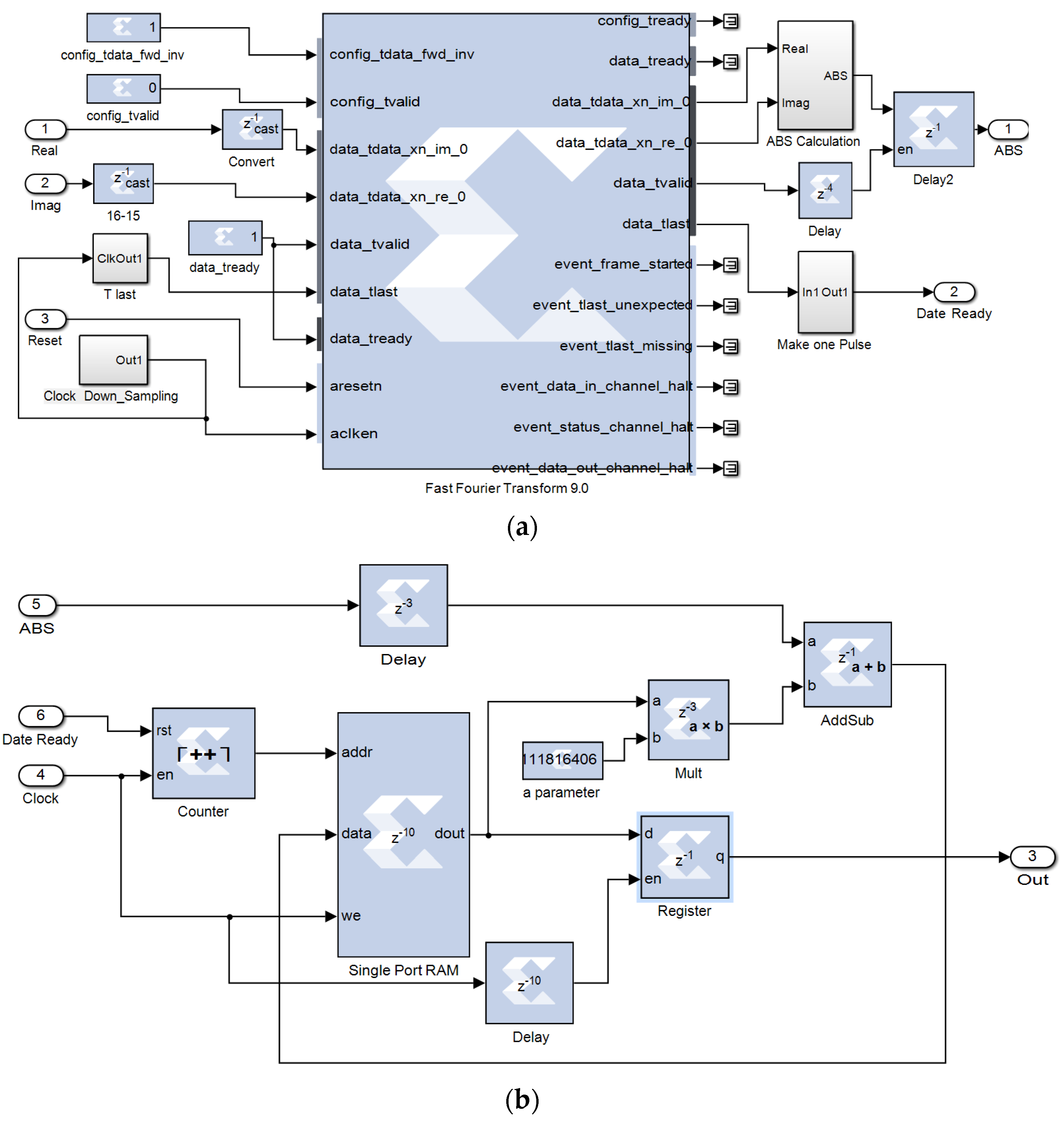
5.1. Design in Xilinx DSP Generator Library

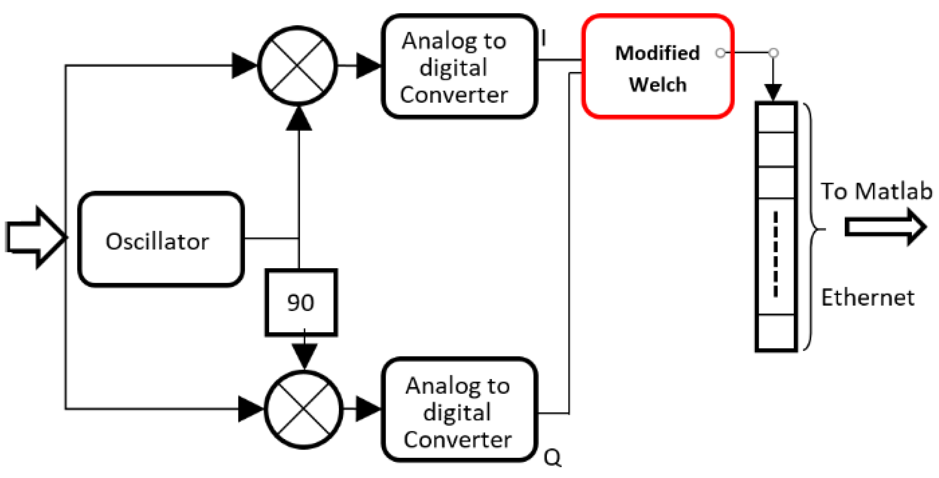
The practical part of this research benefits from the digital signal-processing library provided in the Xilinx System Generator integrated in the Simulink environment. The following methodology contains two main steps: system performance and mathematical discovery based on the simulation that followed by transferring all simulation blocks to the Xilinx DSP Generator. The FFT blocks provided in this library are flexible for multiple FFT sample size adjustments even after synthesis while FPGA is running. The idea is that the method proposed must be practical and easily implementable in the existing technology as much as possible. Following this idea in the simulation design step and benefiting from the Xilinx DSP library, the modified design can easily be transferred from simulation to a worthy FPGA design. Thus, one can assume that the real response of the FPGA design will be reflected accurately in the simulation.

Figure 13a,b represent the most important blocks used in the Xilinx DSP library. The Xilinx Fast Fourier Transform block core computes N-point forward DFT or inverse DFT based on the Cooley-Tukey FFT algorithm [26]. It buffers a vector of N complex values provided on real and imaginary input ports during the N system clocks and generates N_F frequency samples in a series manner on real and imaginary output ports. For synchronization, this block also provides a synchronization signal, the “Data Ready pulse”. This signal simply represents the start and end of each calculated FFT packet. Connecting this pulse to the reset port of a free counter recreates the behavior similar to the simulation step. The second block is the RAM, which is one of the main components of the modified Welch algorithm presented in this paper. The RAM size can also be adjusted to increase or decrease the resolution of the spectral representation. The desired frequency resolution can be easily adjusted with the FTT and RAM size. The smoothness and past value dependency can be set up simply by adjusting the $\alpha$ parameter. These two options give the user unique flexibility for dynamic system adjustment based on the current situation.

Warning: as mentioned before, sorted values inside the RAM will grow to a certain value, then, the system will converge to a final spectrum. The important point here, is the hardware limitation for saving large values inside the RAM. If the averaging value goes higher than the saturation limit of the user computational capability, then an error will be generated. Xilinx DSP generator allows the designer to adjust the precision and “fixed point” output type for each block. For the blocks that are involved in Figure 13, “number of bits” and “binary point” must be selected carefully to avoid the saturation error. During the real time test, hardware limitation must also be considered for selecting the maximum value for the $a$ parameter.

5.2. BEEcube SDR

The NanoBEE device by National Instruments is used as a SDR receiver. This SDR is equipped with a programmable FPGA to implement the algorithm as well as a register bank module to store samples and result data [27].

Once the data is processed, the results are stored inside the register bank, then sent via Ethernet cable to a computer equipped with MATLAB for spectral representation. Figure 14 explains the reception structure of the BEEcube used in this setup. The modified design resides in the Welch block marked in red. It should be mentioned that all the PSD estimation steps are completed in the heart of SDR FPGA, and MATLAB just presents the results stored in the register bank as figures for visualization purposes.

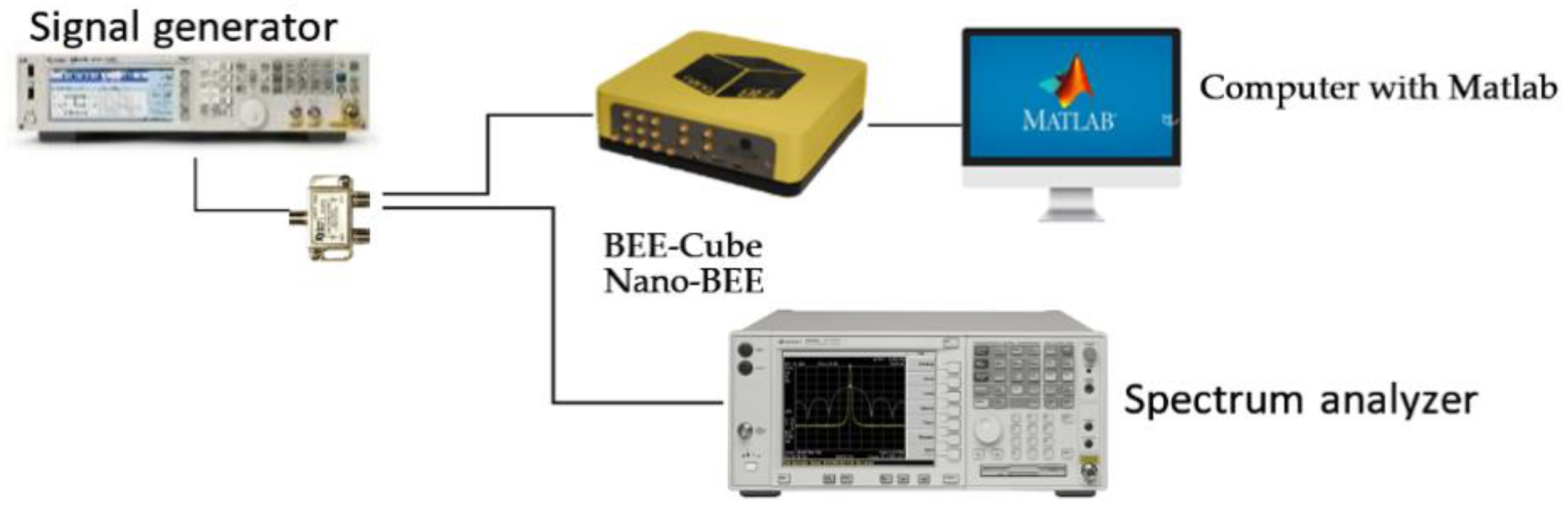
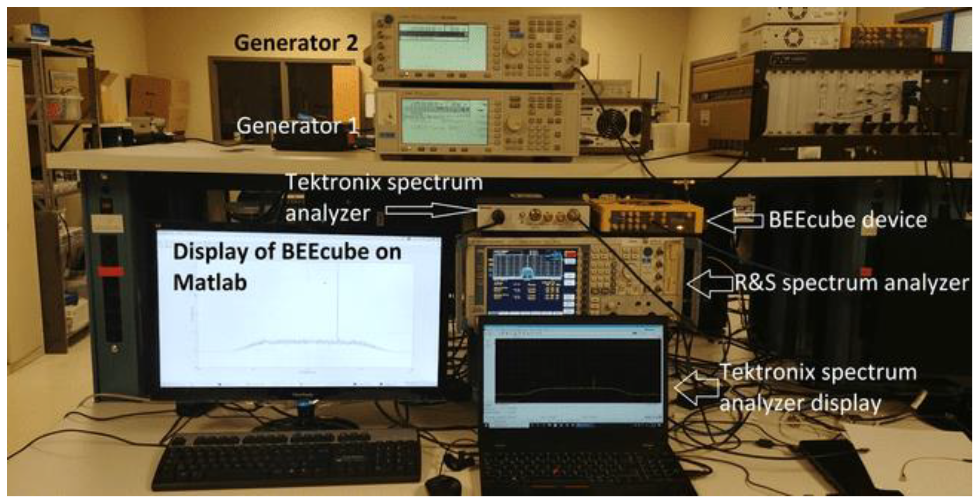
5.3. Practical Setup and Real-Time Test Bench

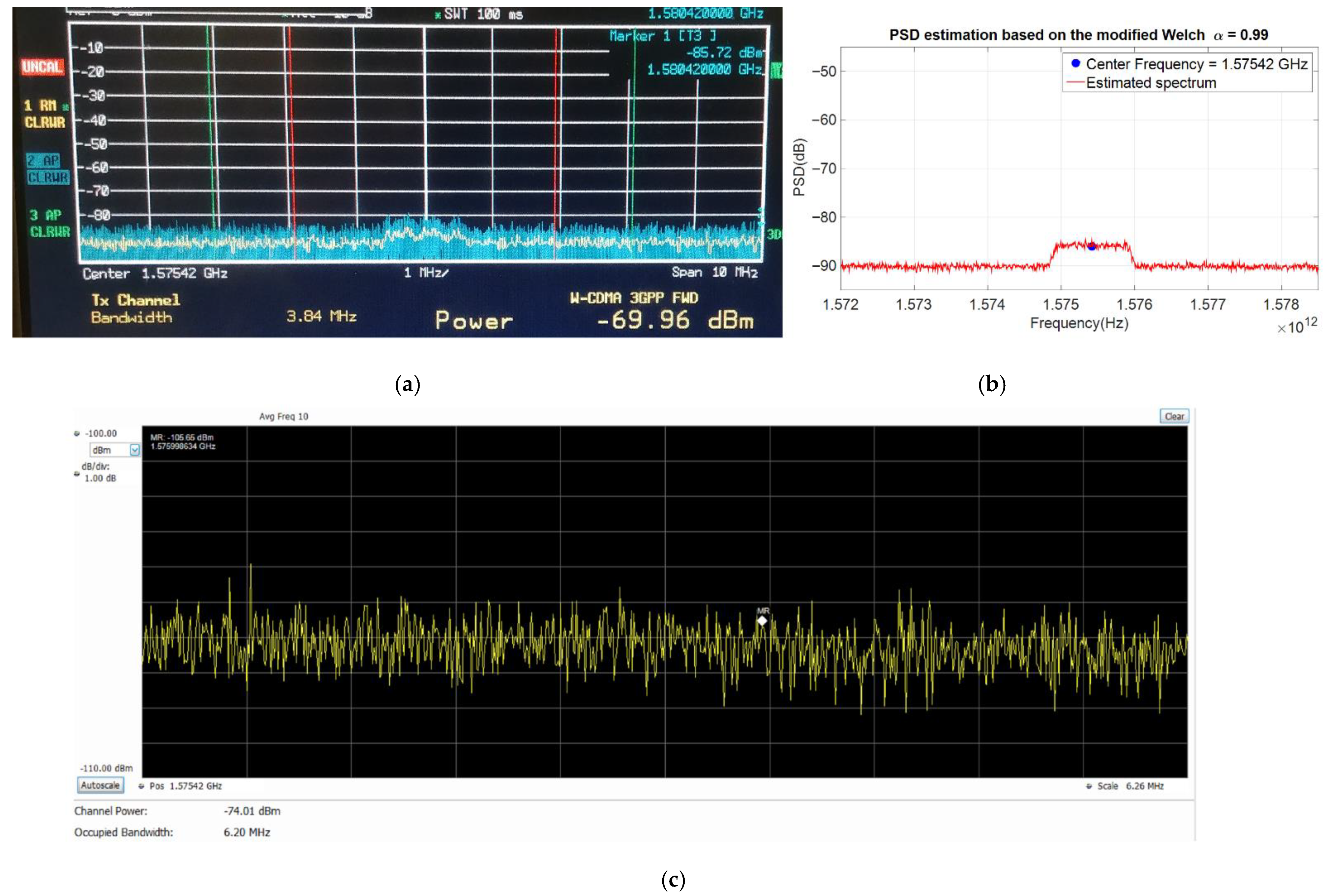
This section tries to validate the proposed algorithm by representing the results obtained in a real-time test bench. The data acquisition and setup are similar to the ones used in [27,28] and with a simulation-based debugging before FPGA synthesis. Use of a software-defined radio (SDR) allowed us to compare the results with reliable standardized spectrum monitoring devices and make a real-time comparison with them. The diagram in Figure 15 and Figure 16 presents the laboratory setup used to validate and compare the algorithm to two standard spectrum monitoring devices. For comparison, two commercially available spectrum monitoring devices from Rohde & Schwarz [29] and Tektronix [30] are used to validate the obtained results. In the case of the Tektronix analyzer, the Long-Term Evolution (LTE) without averaging spectrum analyzer was used to display the signal even more clearly.

5.4. Final Results

The modified design was tested in the laboratory using the setup presented in Figure 16. The first result tries to show the capacity to detect every type of narrow band and wideband signals in different frequencies, like any other spectrum analyzer. A single tone at a frequency of 1.572 GHz and a modulated QAM signal with pulse shaping are selected as narrowband, and wideband signals in different center frequencies are then passed through the commercial spectrum analyzer and SDR equipped with the modified Welch algorithm.

Table 1. Parameters used for the first test.

Single-Tone Center Frequency	Modulated QAM Center Frequency	Modulated QAM Bandwidth	Single-Tone Power	Modulated QAM Power	SDR Sample Rate	$\mathit{a}$ Parameter	FFT Size
1.574 GHz	1.57542 GHz	1 MHz	−48 dBm	−65 dBm	40 MHz	0.99	2048

briefly explains the parameters selected for this test.

In regards to the fairness of competition, we considered the following points carefully:

• It should be mentioned that the power transferred by the signal generator is equally divided between all devices with the help of a splitter. Thus, all devices (SDR and two other spectrum analyzers) are competing with similar input power.
• Selected span for commercial devices is 10 MHz. The SDR that run the new design, has a sampling rate of 40 MHz, thus, the span of the SDR is equal to 20 MHz. Selected span for the two other devices is half of SDR, that allows them to have two times better resolution.
• The attenuation gain for all three devices is equal to 0 dB. It allows the two other spectrum analyzers to have maximum sensitivity to the input signal.
• Selected cables have the same attenuation gain.
• During the test, we also changed the input signal of different devices to be sure that the obtained results were real.

Table 2. Commercial devices parameters.

Rohde & Schwarz
Span	Reference level	Attenuation gain	Center frequency	Resolution bandwidth
10 MHz	0 dB	0 dB	1.57542 GHz	30 kHz
Tektronix RSA600
Span	Reference level	Attenuation gain	Center frequency	Resolution bandwidth
6.2 MHz	−20 dB	0 dB	1.57542 GHz	1 kHz

provide more details about the commercial device settings.

As it can be seen in Figure 17, the modified design can represent any spectral formation with accuracy for signal monitoring and interference detection. For both narrowband and wideband signals, the center frequencies detected match the transferred signals completely, and the bandwidth detected is equal to the bandwidth of the modulated QAM.

The next part of the laboratory results represents the effect of α on the spectrum smoothness and accuracy in frequency component recognition. Figure 18a–c represent a modulated QAM signal at 1.57542 GHz mixed with a CWI at 1.575 GHz compared to the two other spectrum analyzers. In this test, a very low-power CWI is used to make it harder to detect. In this situation, both of the commercial spectrum analyzers could not see the CWI and the modified design was able to detect the spike caused by the interference. Another important point observed in Figure 18 is that the spectrum displayed by the modified design is similar in shape to the two other spectrum analyzers with less noise, and the CWI can appear 4 dB higher than the modulated signal.

Figure 19 represents the results obtained from SDR by repeating the second tests using lower $a$ parameters.

As it can be seen, smother spectrum is obtained for the larger a parameter. The lower the α parameter, the harder it gets to detect the CWI mixed with the modulated QAM until for α = 0.70 in Figure 19b, the CWI peak is covered by noise and is not visible.

The last test tries to compare the ability of two commercial spectrum analyzers with the modified design in weak signal monitoring. In this test, only a wideband signal with low power is used. The signal power transmitted is decreased until the spectrum analyzers are unable to monitor it. As it can be seen in the Figure 20, with a transmitted power of −87 dBm, both spectrum analyzers are unable to monitor the input power, and the transmitted spectrum is covered by noise; however, the SDR equipped with the modified design still clearly depicts signal with correct and reliable details.

For both cases, narrow band and wide band, when other spectrum analyzers could not display the spectrum, the modified design could still display frequency component 5 dB higher than the noise level. With a narrow band signal such as a CWI, when its power is decreased until the point where other devices cannot see the CWI, the new design can see it 5 dB stronger than the QAM signal.

As it has been explained before, α = 0.99 can result in SNR improvement equivalent to averaging by N order of 100. Averaging reduces the noise level and improves the SNR by 20 dB gain. Thus, the frequency components can be visible clearly on top of the noise. Superiority over other spectrum analyzers is demonstrated with the SNR improvement. By decreasing the signal power, it will be fading in the background noise and commercial devices are not able to track it in the surrounding noise. However, the new design, benefiting from the SNR improvement, can display the desired signal in lower SNRs.

5.5. Discussion

The purpose of this paper was to present an easily implementable spectrum monitoring design based on a modified version of the Welch algorithm. The proposed design can accurately represent a low-power signal with a less noisy spectrum reliably when standard spectrum analyzers are unable to track the input signal. Future spectrum monitoring devices such as interference mitigation and detection systems could easily implement this rugged, low-cost and effective design. The unique flexibility allows a lot of different usages such as high-precision spectrum monitoring or high responsiveness for frequency hopping interference tracking. The $\alpha$ parameter helps to have a balance between the required accuracy and the desired convergence in different situations. For instance, the design cannot accurately display a noise-free spectrum while remaining very responsive to frequency hopping. Therefore, there is a trade-off between speed and accuracy when choosing the α value. For future research, the study of this design paired with an interference detection and mitigation device could yield some interesting results. The ability to clearly display low-power interference on top of a noisy signal is very promising for interference mitigation.

Another interesting research would be to adjust the $\alpha$ parameter based on the input signal to noise ratio. The receiver is able to have an approximation of the channel situation and input SNR. Once the receiver is in a good position, selecting a lower $\alpha$ value allows the system to track variable frequency components. While the system is suffering from noisy channel and low SNR, a clearer spectrum curve is available by selecting a larger $\alpha$ parameter.

6. Conclusions

In this research, a modified version of the Welch algorithm for spectrum monitoring is proposed. The characteristics of this design were thoroughly analyzed and studied. Spectrum monitoring is used in multiple applications, from interference mitigation to research and development in the scientific community. After the mathematical explanation and the presentation of the design itself, the effects of the α parameter were presented. It can be concluded that with a smaller α parameter, the system is more responsive and more appropriate for fast hopping frequency signals. On the other hand, with a larger α, the system is more accurate and is more appropriate for precise spectrum monitoring. It is safe to assume that the modified design can reliably and accurately represents any signal type as other commercial devices. From the last results we see that this design can represent low-power signal 5 dB lower than the other standard spectrum analyzers. The proposed algorithm decreases the required space on FPGA and benefiting from its practical design, it can be embedded in SDR or other FPGA core.

The main consideration for this system is the convergence time based on the selected feedback parameter, which can cause loss of information for fast variant frequency components and large values in the RAM component that can generate the saturation error.

References

1. Wu, S.; Feng, L. Design and Implementation of Next Generation Signal Spectrum Monitoring for Satellite Broadcasting Television. In Proceedings of the 2017 4th International Conference on Information Science and Control Engineering (ICISCE), Changsha, China, 21–23 July 2017; pp. 1458–1461. [Google Scholar] [CrossRef]
2. McCarthy, D. Modern Receiver Architectures: Considerations for spectrum monitoring applications. In Proceedings of the 2019 IEEE International Symposium on Electromagnetic Compatibility, Signal & Power Integrity (EMC+SIPI), New Orleans, LA, USA, 22–26 July 2019; pp. 18–21. [Google Scholar] [CrossRef]
3. Ujan, S.; Navidi, N.; Landry, R.J. Hierarchical Classification Method for Radio Frequency Interference Recognition and Characterization in Satcom. Appl. Sci. 2020, 10, 4608. [Google Scholar] [CrossRef]
4. Xu, D.; Zhang, G.; Ding, X. Analysis of Co-channel Interference in Low-orbit Satellite Internet of Things. In Proceedings of the 2019 15th International Wireless Communications & Mobile Computing Conference (IWCMC), Tangier, Morocco, 24–28 June 2019; pp. 136–139. [Google Scholar] [CrossRef]
5. Witte, R.A. Spectrum and Network Measurements; Scitech Publ.: Marina del Rey, CA, USA, 2014. [Google Scholar]
6. Zhao, H.; Lin, G. Nonparametric and parametric methods of spectral analysis. In MATEC Web of Conferences; EDP Sciences: Paris, France, 2019. [Google Scholar]
7. Xu, Q.; Duan, Z. A fixed point of DFT/FFT for FPGA platform. In Proceedings of the 2012 IEEE International Conference on Computer Science and Automation Engineering (CSAE), Zhangjiajie, China, 25–27 May 2012; pp. 279–282. [Google Scholar] [CrossRef]
8. Liavas, A.P.; Moustakides, G.V.; Henning, G.; Psarakis, E.Z.; Husar, P. A periodogram-based method for the detection of steady-state visually evoked potentials. IEEE Trans. Biomed. Eng. 1998, 45, 242–248. [Google Scholar] [CrossRef] [PubMed]
9. Barbe, K.; Pintelon, R.; Schoukens, J. Welch Method Revisited: Nonparametric Power Spectrum Estimation Via Circular Overlap. IEEE Trans. Signal Process. 2010, 58, 553–565. [Google Scholar] [CrossRef]
10. Krishna, A.; Andrews, J. PSD computation using modified Welch algorithm. Int. J. Sci. Res. Eng. Technol. 2015, 4, 951–954. [Google Scholar]
11. Marple, L. A new autoregressive spectrum analysis algorithm. IEEE Trans. Acoust. Speech Signal Process. 1980, 28, 441–454. [Google Scholar] [CrossRef]
12. Bisina, K.V.; Azeez, M.A. Optimized estimation of power spectral density. In Proceedings of the 2017 International Conference on Intelligent Computing and Control Systems (ICICCS), Madurai, India, 15–16 June 2017; pp. 871–875. [Google Scholar] [CrossRef]
13. Welch, P. The use of fast Fourier transform for the estimation of power spectra: A method based on time averaging over short, modified periodograms. IEEE Trans. Electroacoust. 1967, 15, 70–73. [Google Scholar] [CrossRef] [Green Version]
14. Sorensen, H.; Jones, D.; Heideman, M.; Burrus, C. Real-valued fast Fourier transform algorithms. IEEE Trans. Acoust. Speech Signal Process. 1987, 35, 849–863. [Google Scholar] [CrossRef] [Green Version]
15. Hemmert, K.S.; Underwood, K.D. An analysis of the double-precision floating-point FFT on FPGAs. In Proceedings of the 13th Annual IEEE Symposium on Field-Programmable Custom Computing Machines (FCCM’05), Napa, CA, USA, 18–20 April 2005; pp. 171–180. [Google Scholar] [CrossRef]
16. Garg, V.K.; Wang, Y. Data Communication Concepts. In The Electrical Engineering Handbook, 1st ed.; Elsevier: Cambridge, MA, USA, 2005; Chapter 5; pp. 983–988. [Google Scholar]
17. Nussbaumer, H.J. The fast Fourier transform. In Fast Fourier Transform and Convolution Algorithms; Springer: Berlin/Heidelberg, Germany, 1981; pp. 81–111. [Google Scholar]
18. Parhi, K.K.; Ayinala, M. Low-Complexity Welch Power Spectral Density Computation. IEEE Trans. Circuits Syst. I Regul. Pap. 2014, 61, 172–182. [Google Scholar] [CrossRef]
19. Zou, P.; Lv, M. A fast algorithm for blind estimation of frequency domain parameters of Direct Sequence Spread Spectrum signal. In Proceedings of the 2009 IEEE International Conference on Communications Technology and Applications, Beijing, China, 16–18 October 2009; pp. 430–435. [Google Scholar] [CrossRef]
20. Varma, B.S.C.; Paul, K.; Balakrishnan, M. Accelerating 3D-FFT Using Hard Embedded Blocks in FPGAs. In Proceedings of the 2013 26th International Conference on VLSI Design and 2013 12th International Conference on Embedded Systems, Pune, India, 5–10 January 2013; pp. 92–97. [Google Scholar] [CrossRef]
21. John, M.S.; Dimitrijevic, A.; Picton, T.W. Weighted averaging of steady-state responses. Clin. Neurophysiol. 2001, 112, 555–562. [Google Scholar] [CrossRef]
22. Gavaskar, G.R.; Chaudhury, K.N. Fast adaptive bilateral filtering. IEEE Trans. Image Process. 2018, 28, 779–790. [Google Scholar] [CrossRef]
23. Papari, G.; Idowu, N.; Varslot, T. Fast bilateral filtering for denoising large 3D images. IEEE Trans. Image Process. 2016, 26, 251–261. [Google Scholar] [CrossRef] [PubMed]
24. Kovacs, Z.L. On the Enhancement of the SNR of Repetitive Signals by Digital Averaging. IEEE Trans. Instrum. Meas. 1979, 28, 152–155. [Google Scholar] [CrossRef]
25. Same, M.H.; Gandubert, G.; Ivanov, P.; Landry, R.; Gleeton, G. Effects of Interference and Mitigation Using Notch Filter for the DVB-S2 Standard. Telecom 2020, 1, 17. [Google Scholar] [CrossRef]
26. Puschel, M. Cooley-Tukey FFT like algorithms for the DCT. In Proceedings of the 2003 IEEE International Conference on Acoustics, Speech, and Signal Processing, (ICASSP’03), Hong Kong, China, 6–10 April 2003; p. II-501. [Google Scholar] [CrossRef] [Green Version]
27. Ujan, S.; Navidi, N.; Landry, R., Jr. An Efficient Radio Frequency Interference (RFI) Recognition and Characterization Using End-to-End Transfer Learning. Appl. Sci. 2020, 10, 6885. [Google Scholar] [CrossRef]
28. Ujan, S.; Same, M.H.; Landry, R.J. A Robust Jamming Signal Classification and Detection Approach Based on Multi-Layer Perceptron Neural Network. Int. J. Res. Stud. Comput. Sci. Eng. 2020, 7, 1–12. [Google Scholar] [CrossRef]
29. Rohde & Schwarz. R&S®FSQ Signal Analyzer Operating Manual; Operating Manual 1313.9681.12-02; Rohde & Schwarz: Munich, Germany, 2014. [Google Scholar]
30. Tektronix. RSA600 Series Real Time Spectrum Analyzers. Available online: https://www.tek.com/spectrum-analyzer/rsa600-series (accessed on 4 September 2020).
Figure 1. Calculating Welch samples based on the weighted averaging.
Applsci 11 00086 g001
Figure 2. General block diagram of modified design of Welch algorithm implementation.
Applsci 11 00086 g002
Figure 3. A discrete signal (a) without noise (b) with noise Signal to Noise Ratio (SNR) = 15 dB. (c) SNR improvement after arithmetic averaging versus order N. (d) SNR improvement after weighted averaging versus α parameter.
Applsci 11 00086 g003
Figure 4. Frequency representation of the original Welch frequency variation response.
Applsci 11 00086 g004
Figure 5. Frequency representation of the modified Welch frequency variation response.
Applsci 11 00086 g005
Figure 6. Convergence and gain of different a parameter.
Applsci 11 00086 g006
Figure 7. Frequency response of the modified Welch with the correction factor.
Applsci 11 00086 g007
Figure 8. General block diagram of implementation of modified design in Simulink.
Applsci 11 00086 g008
Figure 9. (a) Schematic of the updated Welch algorithm, (b) Fast Fourier Transform (FFT) implementation of modified Welch.
Applsci 11 00086 g009
Figure 10. Amplitude of FFT samples based on the index number (NFFT = 2048).
Applsci 11 00086 g010
Figure 11. Convergence of Welch samples.
Applsci 11 00086 g011
Figure 12. Welch spectrum obtained with different α parameters.
Applsci 11 00086 g012
Figure 13. (a) FFT block from the Xilinx Digital Signal Processing (DSP) Generator library; (b) Random Access Memory (RAM) block from the Xilinx DSP Generator library.
Applsci 11 00086 g013
Figure 14. Nano-BEE reception structure.
Applsci 11 00086 g014
Figure 15. Test bench used to validate the modified algorithm.
Applsci 11 00086 g015
Figure 16. Laboratory setup and devices (signal generators, BEEcube SDR (Software Defined Radio), Tektronix and Rohde & Schwarz) used for real-time analysis.
Applsci 11 00086 g016
Figure 17. (a) CWI (Carrier Wave Interference) represented and QAM (Quadrature Amplitude Modulation) modulated with the R&S (Rohde & Schwarz) spectrum analyzer; (b) CWI represented and QAM signal spectrum modulated with the modified Welch algorithm.
Applsci 11 00086 g017
Figure 18. (a) CWI and modulated QAM signal representation on the R&S spectrum analyzer; (b) CWI and modulated QAM signal representation with the modified Welch algorithm with α = 0.99 (c) CWI and modulated QAM signal representation with the Tektronix spectrum analyzer.
Applsci 11 00086 g018
Figure 19. (a) CWI and modulated QAM signal representation with α = 0.85; (b) CWI and modulated QAM signal representation with α = 0.7.
Applsci 11 00086 g019
Figure 20. (a) PSD representation from the R&S spectrum analyzer at −87 dBm; (b). PSD representation from the modified Welch algorithm at −87 dBm; (c) PSD representation from the Tektronix spectrum analyzer at −87 dBm.
Applsci 11 00086 g020